


Abstract
Extremal graphical models are sparse statistical models for multivariate extreme events. The underlying graph encodes conditional independencies and enables a visual interpretation of the complex extremal dependence structure. For the important case of tree models, we develop a data-driven methodology for learning the graphical structure. We show that sample versions of the extremal correlation and a new summary statistic, which we call the extremal variogram, can be used as weights for a minimum spanning tree to consistently recover the true underlying tree. Remarkably, this implies that extremal tree models can be learned in a completely non-parametric fashion by using simple summary statistics and without the need to assume discrete distributions, existence of densities or parametric models for bivariate distributions.
1 INTRODUCTION
Extreme value theory provides essential statistical tools to quantify the risk of rare events such as floods, heatwaves or financial crises (e.g. Engelke et al., 2019; Katz et al., 2002; Poon et al., 2004). The univariate case is well understood and the generalised extreme value and Pareto distributions describe the distributional tail with only few parameters. In dimension , the dependence between large values in the different components of a random vector can become very complex. Estimating this dependence in higher dimensions is particularly challenging because the number of extreme observations is by definition much smaller than the number of all samples in a data set. Constructing sparse models for the multivariate dependence between marginal extremes is therefore crucial for obtaining tractable and reliable methods in multivariate extremes; see Engelke and Ivanovs (2021) for a review of recent advances.
One line of research aims at exploiting conditional independence structures (Dawid, 1979) and corresponding graphical models. In the setting of max-stable distributions, which arise as limits of component-wise block maxima of independent copies of , Gissibl and Klüppelberg (2018) and Klüppelberg and Lauritzen (2019) study max-linear models on directed acyclic graphs. The distributions considered in there do not have densities, and a general result by Papastathopoulos and Strokorb (2016) shows that there exist no non-trivial density factorisation of max-stable distributions on graphical structures.
A different perspective on multivariate extremes is given by threshold exceedances and the resulting class of multivariate Pareto distributions. Such distributions are the only possible limits that can arise from the conditional distribution of given that it exceeds a high threshold (Rootzén et al., 2018; Rootzén & Tajvidi, 2006). For a -dimensional random vector that follows a multivariate Pareto distribution, Engelke and Hitz (2020) introduce suitable notions of conditional independence and extremal graphical models with respect to a graph . They further show that these notions are natural as they imply the factorisation of the density of through a Hammersley–Clifford type theorem. Extremal graphical models are also related to limits of regularly varying Markov trees studied in Segers (2020) and Asenova et al. (2021).
In most of the above work, the graphical structure is assumed to be known a priori. It is either based on expert knowledge in the domain of application or it might be identified with an existing graph, as for instance a river network for discharge measurements. However, often no or insufficient domain knowledge on a prior candidate for a graphical structure is available, and a data-driven approach should be followed in order to detect conditional independence relations and to estimate a sensible graph structure. In this work we discuss structural learning for extreme observations.
An important sub-class of general graphs for which structure learning for extremes turns out to be possible in great generality is given by trees. A tree with nodes and edge set is a connected undirected graph without cycles. Most structure learning approaches for trees are based on the notion of the minimum spanning tree. For a set of symmetric weights associated with any pair of nodes , , the latter is defined as the tree structure
that minimises the sum of distances on that tree. Given the set of weights, there exist greedy algorithms that constructively solve this minimisation problem (Kruskal, 1956; Prim, 1957).
The crucial ingredient for this algorithm are the weights between the nodes, and for statistical inference it is generally desirable to choose them in such a way that recovers the true underlying tree structure that represents the conditional independence relations. A common approach in graphical modelling is to use the Chow–Liu tree (Chow & Liu, 1968), which is the conditional independence structure that maximises the likelihood for a given parametric model (cf, Cowell et al., 2006, chapter 11). This method uses the negative mutual information as edge weights in (1), and in general this requires formulating parametric models for the bivariate marginal distributions. In the Gaussian case the weights then simplify to , where are the correlation coefficients (cf, Drton & Maathuis, 2017).
For a multivariate Pareto distribution that is an extremal graphical model on a tree , Engelke and Hitz (2020) proposed to use the negative maximised bivariate log-likelihoods as edge weights. This approach has two disadvantages. First, in higher dimensions it may become prohibitively costly to compute censored likelihood optimisations, and second, a set of parametric bivariate models has to be chosen in advance.
In this paper we study structure learning for extremal tree models in much larger generality. We show that a function of the extremal correlation , a widely used coefficient to summarise the strength of extremal dependence between marginals (e.g., Coles et al., 1999), can be used as weights in (1) to retrieve the underlying tree structure as the minimum spanning tree under mild non-parametric assumptions. We further introduce a new summary coefficient for extremal dependence, the extremal variogram , which turns out to take a similar role in multivariate extremes as covariances in Gaussian models. More precisely, the extremal variogram of is shown to be an additive tree metric on the tree and, as a consequence, it can be used as well as weights of the minimum spanning tree to recover the true tree structure. Surprisingly, these results are stronger than for non-extremal tree structures, since we do not require any further parametric assumptions or the existence of densities. This phenomenon originates from the homogeneity of multivariate Pareto distributions and particularly nice stochastic representations of extremal tree models.
In practice, we usually observe samples of in the domain of attraction of , that is, the conditional distribution of given exceeds a high threshold converges to the distribution of after proper scaling; see Section 2.1 for a formal definition. We then rely on estimators of the quantities and to plug into (1). To take into account that is only in the domain of attraction of , typical estimators in extreme value theory use only the most extreme observations. We use an existing estimator of extremal correlation and a new empirical estimator of the extremal variogram to show that the extremal tree structure can be estimated consistently in a non-parametric way, even when the dimension increases with the sample size.
The remaining paper is organised as follows. In Section 2 we revisit the notion of extremal graphical models and extend existing representations to the case where densities may not exist. The extremal variogram is introduced in Section 3 and its properties are discussed in detail. In Section 4 we prove the main results on the consistent recovery of extremal tree structures based on extremal correlations and extremal variograms, both on the population level and using empirical estimates. The simulation studies in Section 5 illustrate the finite sample behaviour of our structure estimators and show that extremal variogram based methods typically outperform methods working with the extremal correlation. We apply the new tools in Section 6 to a financial data set of foreign exchange rates. The Appendix and the Supplementary Material S1 contain the proofs and additional illustrations. The methods of this paper are implemented in the R package graphicalExtremes (Engelke et al., 2019).
2 EXTREMAL GRAPHICAL MODELS
2.1 Multivariate Pareto distributions
Let be a random vector with eventually continuous marginal distribution functions . Extreme value theory studies marginal and joint tail properties of . Univariate extreme value theory focuses on the behaviour of marginal components , see for example Embrechts et al. (1997) and Coles et al. (1999). Multivariate extreme value theory is concerned with the dependence structure among different components of extreme observations from ; see Resnick (2008, chapter 5); de Haan and Ferreira (2006); Beirlant et al. (2004) or Engelke and Ivanovs (2021) for an introduction.
One way to describe such tail properties is based on threshold exceedances; here only observations that land above a high threshold are considered. Multivariate Pareto distributions arise as the limits of such high threshold exceedances and are thus natural models for extreme events (Rootzén & Tajvidi, 2006). To formally define threshold exceedances in dimension , we need to specify the notion of a high threshold in a multivariate setting. Throughout the paper, we consider multivariate exceedances of the random vector as those realisations where at least one component of exceeds a high marginal quantile. In order to guarantee the existence of the limit of the exceedance distribution, a regularity condition called multivariate regular variation (Resnick, 2008, Chapter 5) is needed. Intuitively, this assumption ensures that the dependence between different components of this conditional distribution stabilises if the marginal quantile is sufficiently large. More formally, this means that there exists a random vector supported on such that for all continuity points of the distribution function of we have
where we define . Note that the condition states that at least one component of exceeds its marginal quantile, explaining the terminology of threshold exceedances. Distributions of random vectors that can arise in the above limit are called multivariate Pareto distributions. We say that the random vector is in the max-domain of attraction of the multivariate Pareto distribution .
The class of multivariate Pareto distributions is very general and contains many different parametric sub-families. Nevertheless, since the random vector arises as a limiting distribution, it has an important structural property called homogeneity:
where for any Borel subset we define . This explains the name multivariate Pareto distribution since it implies that for any we have for , that is, follows a standard Pareto distribution. Moreover, since has identically distributed margins, it follows from (2) that . Conversely, if the latter holds and is homogeneous as in (3), then is a multivariate Pareto distribution; for a proof of this equivalence and the relationship to limits appearing in Segers (2020) see Section S.5 of Supplementary Material S1.
2.2 Extremal Markov structures
Since the support of multivariate Pareto distributions is not a product space, the definition of conditional independence is non-standard and relies on auxiliary random vectors derived from . For any , we consider the random vector defined as conditioned on the event that , which has support on the space . For general random vectors and ordered sets , let denote the sub-vector of with indices in . The notation will be used to denote the subvector of with indices in .
With this notation we can state a definition of conditional independence for multivariate Pareto distributions that is more general than the one in Engelke and Hitz (2020), since we do not assume existence of densities.
Definition 1For disjoint subsets , we say that is conditionally independent of given if
(4)In this case we write .
The subscript in indicates that this conditional independence notion is defined for extreme observations, which are described by the multivariate Pareto distribution according to (2).
We view the index set as a set of nodes of a graph , with connections given by a set of edges of pairs of distinct nodes. The graph is called undirected if for two nodes , if and only if . For notational convenience, for undirected graphs we sometimes represent edges as unordered pairs . When counting the number of edges, we count such that each edge is considered only once. For disjoint subsets , is said to separate and in if every path from to contains as least one node in . For an illustration of these definitions see Section S.1 in Supplementary Material S1.
The notion of an extremal graphical model is then naturally defined as a multivariate Pareto distribution that satisfies the global Markov property on the graph with respect to the conditional independence relation , that is, for any disjoint subsets such that separates from in ,
In line with the definition in the graphical models literature (Lauritzen, 1996, chapter 3), the definition allows for additional conditional independence relations that are not encoded by graph separation. This means that there are typically several graphs that are consistent with the distribution of ; for instance, any multivariate Pareto distribution is an extremal graphical model on the fully connected graph.
In the case of a decomposable graph and if possesses a positive and continuous density , Engelke and Hitz (2020) show that this density factorises into lower-dimensional densities, and that the graph is necessarily connected. If does not have a density, then the extremal graph can be disconnected and the connected components are mutually independent of each other (Engelke & Hitz, 2020, see Kirstin Strokorb's discussion contribution). Note that we require the global Markov property in the definition of extremal graphical models as opposed to the pairwise Markov property used in Engelke and Hitz (2020). Both properties are equivalent in the case of positive, continuous densities, but in general, the former implies the latter but not the other way around (see Lauritzen, 1996, chapter 3).
2.3 Extremal tree models
An important example of a sparse graph structure is a tree. A tree is a connected undirected graph without cycles and thus . Equivalently, a tree is a graph with a unique path between any two nodes. If is an extremal graphical model satisfying the global Markov property (5) with respect to a tree , we obtain a simple stochastic representation of . This stochastic representation will be the crucial building block for the results on tree learning given in the next section.
To this end we need to introduce the concept of extremal functions. Define the extremal function relative to coordinate as the -dimensional, non-negative random vector with almost surely that satisfies the stochastic representation
where is a standard Pareto random variable, , , which is independent of , and stands for equality in distribution. Such a representation is possible by homogeneity (3) of , which is inherited by . Indeed, given homogeneity of we see that follows a standard Pareto distribution. Moreover, writing , homogeneity of and a simple calculation implies that and are independent, resulting in the representation (6).
The representation (6) is an alternative way of describing the distribution of , and indeed, the set of the extremal functions uniquely defines the multivariate Pareto distribution. We refer to Dombry et al. (2013, 2016) for additional technical background on extremal functions.
Example 1In the case , due to homogeneity, the bivariate Pareto distribution can essentially be characterised by a univariate distribution. Indeed, for any non-negative random variable with , the random vector is the extremal function relative to the first coordinate of a unique bivariate Pareto distribution . The extremal function relative to the second coordinate is obtained through a change of measure
(7)which implies that .
An elementary proof of (7) can be found in Section S.7 of Supplementary Material S1.
We now proceed to a stochastic representation for that involves only the univariate random variables . Define a new, directed tree rooted at an arbitrary but fixed node . The edge set consists of all edges of the tree pointing away from node . For the resulting directed tree we define a set of independent random variables, where for , the distribution of is th coordinate of the extremal function of relative to coordinate .
The following result generalises proposition 2 in Engelke and Hitz (2020) to extremal tree models with arbitrary edge distributions.
Proposition 1Letbe a multivariate Pareto distribution that is an extremal graphical model on the tree. Letbe a standard Pareto distribution, independent of. Then we have the joint stochastic representation foron
(8)wheredenotes the set of edges on the unique path from nodeto nodeon the tree; see Figure1for an example with.
Conversely, for any set of independent random variables, whereandsatisfy the duality (7), the construction (8) defines a consistent family of extremal functionsthat correspond to a unique-dimensional Pareto distributionthat is an extremal graphical model on.
![A tree T2 rooted at node m=2 with the extremal functions on the edges [Colour figure can be viewed at https://dbpia.nl.go.kr]](https://oup.silverchair-cdn.com/oup/backfile/Content_public/Journal/jrsssb/84/5/10.1111_rssb.12556/1/m_rssb_84_5_2055_fig-1.jpeg?Expires=1750325314&Signature=dYn7L0f~qxb~W4X0YohYsD09tuMywcBIyJtU8ZH4OPc8YO7EUYhRnRsti2Xu-AbZFZGyFrxDDQBuQbau2hRLiQNV6VhzGAT1eTKZRVOWVqxMnnZs7Ob0Xct4dPflH7QFMXqIZaHQG38PM65Xb-PSABGKK6UoW2qg-nNo-OSGkUQbYjVZQTGQ~mpG8PlBnaf8ROKj6rVlIQWf4cBRb0pBvi~r94V7BT2w1h9PgI5kIUSi06twkAZjqbnHXzUMhyJWdEJi3jSNYh2Z0bh3bHK3o4QMtum~F-3xzbpzBoZ1t7iwyPy~f1ZFeW~c51A11-86WMyJ4vGTiMiu~WePv5rGVQ__&Key-Pair-Id=APKAIE5G5CRDK6RD3PGA)
A tree rooted at node with the extremal functions on the edges [Colour figure can be viewed at https://dbpia.nl.go.kr]
The above result formally establishes the link of the conditional independence in Definition 1 to the limiting tail trees in Segers (2020); see also Proposition 1 in Supplementary Material S1 for details on this link. In this sense, the first part of Proposition 1 can be deduced from theorem 1 in Segers (2020).
Note that defined as in Proposition 1 can also be an extremal graphical model on a disconnected graph ; see the paragraph after (5). The representation (8) then remains true and some of the are almost surely equal to zero.
Remark 1It is remarkable that for an extremal tree model , the distribution of its extremal functions, and therefore also of the multivariate Pareto distribution itself, is characterised by the set of univariate random variables . This indicates that the probabilistic structure is simpler than in the non-extremal case, where in general both univariate and bivariate distributions are needed to describe a tree graphical model.
3 THE EXTREMAL VARIOGRAM
Covariance matrices play a central role in structure learning for Gaussian graphical models due to their connection to conditional independence properties. In multivariate extreme value theory, several summary statistics have been developed to measure the strength of dependence between the extremes of different variables. The most popular one is the extremal correlation, which for is defined as
whenever the limit exists. It ranges between 0 and 1 where the boundary cases are asymptotic independence and complete extremal dependence, respectively (cf, Coles et al., 1999; Schlather & Tawn, 2003). In particular, if is in the max-domain of attraction of the multivariate Pareto distribution , then the extremal correlation always exists and . There are many other coefficients for extremal dependence in the literature, including the madogram (Cooley et al., 2006) and a coefficient defined on the spectral measure introduced in Larsson and Resnick (2012) and used for dimension reduction in Cooley and Thibaud (2019) and Fomichov and Ivanovs (2022).
While designed as summaries for extremal dependence, none of these coefficients has an obvious relation to conditional independence for multivariate Pareto distributions or density factorisation in extremal graphical models of Engelke and Hitz (2020). In this section we define a new coefficient that will turn out to take a similar role in multivariate extremes as covariances in non-extremal models.
3.1 Limiting extremal variogram
The variogram is a well-known object in geostatistics that measures the degree of spatial dependence of a random field (cf, Chilès & Delfiner, 2012; Wackernagel, 2013). It is similar to a covariance function, but instead of positive definiteness, a variogram is conditionally negative definite; for details, see for instance Engelke and Hitz (2020, Appendix B). For Brown–Resnick processes, the seminal work of Kabluchko et al. (2009) has shown that negative definite functions play a crucial role in spatial extreme value theory. We define a variogram for general multivariate Pareto distributions.
Definition 2For a multivariate Pareto distribution we define the extremal variogram rooted at node as the matrix with entries
(10)whenever the right-hand side exists and is finite.
We can interpret the as a distance between the variables and that is large if their extremal dependence is weak and vice versa.
Proposition 2Letbe a multivariate Pareto distribution.
- (i)
For, we can express the extremal variogram in terms of the extremal function relative to coordinate,- (ii)
For, the matrixis a variogram matrix, that is, it is conditionally negative definite.
- (iii)
Letbe a sequence of multivariate Pareto distributions with extremal coefficientsbetween theth andth coordinate ofsatisfyingasfor some. Then the corresponding extremal variograms satisfyas.
Part (iii) in the above proposition underlines the interpretation of the extremal variogram. When the variables become asymptotically independent, then the extremal variogram grows and eventually diverges to . Note that the converse statement is not true in general, since there are cases where but . We proceed with several examples where the extremal variogram can be computed explicitly. Figure 2 shows the extremal variogram values for these models as a function of the corresponding extremal correlation.
![Values of the extremal variogram Γ12(1) as a function of the extremal correlation χ12 for the bivariate Hüsler–Reiss (blue), symmetric Dirichlet (orange) and logistic (green) models. Note that in all three cases we have that W12=(d)W21 and therefore Γ12(1)=Γ12(2). [Colour figure can be viewed at https://dbpia.nl.go.kr]](https://oup.silverchair-cdn.com/oup/backfile/Content_public/Journal/jrsssb/84/5/10.1111_rssb.12556/1/m_rssb_84_5_2055_fig-2.jpeg?Expires=1750325314&Signature=4vVCJ8-alta-OSHjAC0ZiYCzZmhctmeIjT~eOklfjz2QKatHfw3OI7F3Pq9jutWCAf9iCbgNSWqrLWnpaGuqReT9KXmmOhmHGHSf72ic0ZM8KsbBBu-aV6P0IaYDY04nB-bH4aXUQyQMZBito1~8B4UKtxsPDjdbNAyMc~scCtNLhfNlpcnhJZX6GOUsmrczRZHWBvMbEWJed71IZdKGN5-wk~2H-BnlNpLqUhW9822f5PEPaUhxaFQocHnx5TZZr~0SKr74JX0V8OK564cSeorJVuyhcJe-ngcjbtxS-TczvQweebj0WQhC32VSnnNyMj~1meZ980DEAR13TNxjMQ__&Key-Pair-Id=APKAIE5G5CRDK6RD3PGA)
Values of the extremal variogram as a function of the extremal correlation for the bivariate Hüsler–Reiss (blue), symmetric Dirichlet (orange) and logistic (green) models. Note that in all three cases we have that and therefore . [Colour figure can be viewed at https://dbpia.nl.go.kr]
Example 2The extremal logistic distribution with parameter can be defined through its extremal functions (see Dombry et al., 2016)
where are independent and , follow distributions, and follows a distribution; here is the Gamma function evaluated at . It turns out that for the logistic model we have
where is the trigamma function defined as the second derivative of the logarithm of the gamma function.
The corresponding extremal correlations have the form , .
The proof of this representation of the extremal variogram in the logistic model can be found in Section S.8 in Supplementary Material S1.
Example 3The extremal Dirichlet distributions with parameters (cf, Coles & Tawn, 1991) has extremal functions
where are independent and , follow distributions, and follows a distribution. By straight-forward calculations,
with denoting the trigamma function as in Example 2.
The corresponding extremal correlations do have have a closed form but can be calculated numerically.
For the class of Hüsler–Reiss distributions the extremal variogram turns out to be very natural.
Example 4The Hüsler–Reiss distribution is parameterised by a variogram matrix ; see Engelke and Hitz (2020) for details. For any -variate centred normal random vector with variogram matrix , the extremal function relative to coordinate has representation
(11)see Dombry et al. (2016, prop. 4). The extremal variogram for any is then equal to the variogram matrix from the definition of the Hüsler–Reiss distributions, and, in particular, it is independent of the root node,
The corresponding extremal correlations have the form , where is the standard normal distribution function.
3.2 Pre-asymptotic extremal variogram
Similar to the extremal correlation in (9) we can define the extremal variogram as the limit of pre-asymptotic versions.
Definition 3For a multivariate distribution with continuous marginal distributions we define the pre-asymptotic extremal variogram at level rooted at node as the matrix with entries
whenever right-hand side exists and is finite.
Note that for close to zero the conditional distribution of the terms given is approximately that of , .
Next we provide conditions which ensure the convergence as . We introduce the following notation: for a vector and , let denote a vector in with entries . For a distribution function of a -dimensional random vector define as the distribution function of the corresponding random vector and let denote the limit obtained in relation (2) when are replaced by . Note that is not the same as , the sub-vector of with entries in , because the latter is not supported on . The distribution of can be obtained from that of by conditioning.
- (B)There exist constants such that for any with and all(12)
- (T)There exists a such that for any the extremal function satisfies(13)
Assumption (B) is a strengthening of (2) for bivariate and trivariate distributions as it imposes that convergence to the limit should take place uniformly and at a certain rate. It is closely related to typical second order conditions on the stable tail dependence function that are fairly standard in the literature; see for instance Einmahl et al. (2012) and Fougères et al. (2015) among many others. Additional details on this matter are given in the Section S.12.1 in Supplementary Material S1. Condition (T) is a mild assumption on the extremal functions , which holds for all examples considered in the previous section. This condition prevents the distribution of from putting too much mass close to zero.
Proposition 3Under conditions (B), (T) we have for any
We note that condition (T) already implies that for any , so the convergence above is always to a finite limit.
4 STRUCTURE LEARNING FOR EXTREMAL TREE MODELS
4.1 Extremal tree models
Extremal graphical models where the underlying graph is a tree were considered as a sparse statistical model in Engelke and Hitz (2020). As explained in the introduction, their approach of using a censored maximum-likelihood tree becomes prohibitively costly in higher dimension and requires parametric assumptions on the bivariate distributions of the tree.
Ideally, one would like to have summary statistics, similar to the correlation coefficients in the Gaussian case, that can be estimated empirically and that guarantee to recover the true underlying tree structure when used as edge weights. The extremal variogram defined in Section 3 turns out to be a so-called tree metric, and as such a natural quantity to infer the conditional independence structure in extremal tree models. We underline that the extremal variogram is defined for arbitrary multivariate Pareto distributions and in the case of the Hüsler–Reiss distribution it coincides with the parameter matrix.
Proposition 4Letbe an extremal graphical model with respect to the treeand suppose that the extremal variogram matrixexists for all. Then we have that
(14)In other words, for any, the extremal variogram matrixdefines an additive tree metric.
Corollary 1Letbe an extremal graphical model with respect to the tree. Suppose that the extremal variogram matrixexists and is finite for alland thatfor all, (or equivalently, ). For any, the minimum spanning tree withis unique and satisfies
For extremal tree models, Corollary 1 shows that independently of any distributional assumption, the extremal variogram contains the conditional independence structure of the tree . This result is quite surprising, since it is stronger than what is known in the classical, non-extremal theory of trees. Indeed, as discussed in the introduction, for Gaussian graphical models, a analogous result holds for a minimum spanning tree with weights for denoting the correlation between the th and th component of the Gaussian random vector under consideration. The assumption of Gaussianity is crucial and the result no longer holds outside this specific parametric class.
Beyond the world of Gaussian graphical models, there exists some literature on the non-parametric estimation of graphical models on tree structures, see Chow and Liu (1968) for an early contribution and Drton and Maathuis (2017, section 3.1) for an overview. However, one either needs to assume discrete distributions (Chow & Liu, 1968) or the existence of densities (Lafferty et al., 2012; Liu et al., 2011), and non-parametric density estimation is required in the latter case. To the best of our knowledge, multivariate Pareto distributions are the first example for a non-parametric sub-class of multivariate distributions where tree dependence structures can be learned using simple moment-based summary statistics without additional parametric assumptions. It is also remarkable that there is no need to assume the existence of densities and that the distributions we consider can simultaneously have continuous and discrete components.
The reason why such a strong result can hold can be explained by the homogeneity of the multivariate Pareto distribution . For trees, all cliques contain two nodes and therefore the density factorises into bivariate Pareto densities. Because of the homogeneity, such a bivariate density can be decomposed into independent radial and angular parts; see Example 1. Bivariate Pareto distributions only differ in terms of the angular distribution, whose support is the subset of a one-dimensional sphere with all coordinates positive. Consequently, an extremal tree model in dimensions can essentially be reduced to univariate angular distributions; see also Proposition 1. This provides an intuitive explanation why the result in Corollary 1 can hold.
We can go further and show that a linear combination of the matrices , , which are possibly different from each other, still induces the true tree as the minimum spanning tree.
Corollary 2Under the same assumptions as in Corollary1, the minimum spanning tree with distances
given by a linear combination of the extremal variograms rooted at different nodes with coefficients, , , is unique and satisfies
The extremal correlation coefficients do not form a tree metric, that is, they are not additive according to the tree structure as the extremal variogram in (A4). It is therefore a non-trivial question whether these coefficients can also be used as weights in a minimum spanning tree to infer the underlying conditional independence structure. Interestingly, the next result gives a partially affirmative answer.
Proposition 5Letbe an extremal graphical model on the tree. Then the extremal correlation coefficients satisfy for anywiththat
(15)Under the additional assumption that this inequality is strict as soon as, the minimum spanning tree corresponding to distancesis unique and satisfies
The assumption that for any with is not satisfied for all tree models. Indeed, a counterexample (Segers, J. [Personal communication, 7th July 2022]) with index set and edges is the following. Let the extremal function and let have a discrete distribution and ; both are valid extremal functions as in Example 1. In this case and the set of minimum spanning trees is not unique. We can then only guarantee that the true underlying tree lies in the set of all possible minimum spanning trees; this follows from a close inspection of the proof of Proposition 5.
There are simple conditions to ensure that inequality (15) is strict for all . For instance, a sufficient condition for this to hold is that all extremal functions for have support equal to the whole space ; see Lemma 1 in Section S.10 in Supplementary Material S1. This covers many relevant examples such as the Hüsler–Reiss, the extremal logistic and the extremal Dirichlet distributions in Examples 2, 3 and 4, respectively. A weaker condition for strict inequality was recently obtained by Hu et al. (2022).
Remark 2Both the extremal variogram and the extremal correlation contain information on conditional independence structure for extremal tree models. The extremal correlation is defined for any model but needs additional assumptions to correctly recover the tree. The extremal variogram does not exist if has mass on lower-dimensional sub-faces of but is guaranteed to recover the underlying tree whenever all extremal variograms exist. When their sample versions are used (see Section 4.2), the probability of correctly identifying the underlying tree may differ even when both approaches work on population level; see Section 5.
4.2 Estimation
Throughout this section assume that we observe independent copies of the -dimensional random vector , which is in the max-domain of attraction of a multivariate Pareto distribution , an extremal graphical model on the tree according to (5). Our aim is to estimate from the observations . Motivated by Proposition 5 and Corollaries 1, 2 we propose to achieve this through a two-step procedure. We first construct estimators for the quantities and , and then compute the minimal spanning trees corresponding to those estimators.
The empirical estimator for is defined as
where is an intermediate sequence and denotes the empirical distribution function of . Standard arguments imply that under (2) and provided that and as , we have for any
where is defined in (9) and . In particular, if then is a consistent estimator of .
The extremal variogram matrix for the sample , , is estimated by
where denotes the sample variance. Under the assumption as and mild conditions on the underlying data generation, this estimator can be shown to be consistent for the pre-asymptotic version as introduced in Definition 3.
Theorem 1Let assumptions (B), (T) hold and assume thatfor someand thatas. Then we have for any
where.
The proof of this result turns out to be surprisingly technical, details are given in the Section S.12.4 in Supplementary Material S1. The main challenge arises from the fact that in the definition of only the observations in component are extreme while observations in other components may also be non-extreme. This is different from the setting that is typically considered in asymptotically dependent extreme value theory.
Remark 3By choosing , the above theorem implies consistency of the empirical extremal variogram . This result is of independent interest, since it is the first proof of consistency of the moment estimators
which were introduced in Engelke et al. (2015) as estimators for the parameters of the Hüsler–Reiss distribution.
Remark 4The assumption that the data are independent was only made to keep the presentation simple. The consistency result in Theorem 1 continues to hold under a high-level assumption that allows for temporal dependence and is spelled out in detail at the beginning of Section S.12.4 in Supplementary Material S1.
Now we have all results that are needed for consistent estimation of the underlying tree structure. Given a general distance with estimator on pairs , we consider plug-in procedures of the form
with three cases of particular interest given by
resulting in the estimators , respectively. The special case of is denoted by . We solve the minimum spanning tree problem (17) by Prim's algorithm, which is guaranteed to find a global optimiser of problem (17) that is unique if the distances are distinct for all pairs (Prim, 1957).
Theorem 2Assume thatis an extremal graphical model on the tree. Assume (2) holds and that the inequality in (15) is strict whenever. Ifasthen there existssuch that under the additional assumptionas,
If instead of (2) and strict inequality in (15) assumptions (B), (T) hold, for all, (or equivalently, ), and iffor somethen for anythere existssuch that foras, we have
The same is true forprovided the weightssatisfy.
Remark 5As pointed out by a referee, it would be of interest to find weights that maximise (asymptotically) the probability of correct tree structure recovery by . This would require precise information on the joint asymptotic distribution of for different , which is currently an open question.
Remark 6At first glance it might seem surprising that the tree structure can be estimated consistently even when does not converge to zero. The latter would be a classical minimal assumption in extreme value theory and would be required for consistent estimation of or . We explain the intuition behind this result for the extremal correlation, the arguments for the extremal variogram are exactly the same. Assume that the inequality in (15) is strict whenever , making the minimal spanning tree with respect to unique. The key insight is that even biased estimators of can lead to the correct minimal spanning tree since all we need is
for all trees , where denotes the true underlying tree. Multivariate regular variation (2) implies that as for all , so there exists such that the above inequality is satisfied for all . Since in addition as under the assumption , consistency follows.
Theorem 2 shows that the proposed procedures are able to consistently recover the tree structure under rather weak assumptions on the sequence . It is natural to wonder which choices of correspond to higher probabilities of recovering the tree structure consistently. Here we provide some indicative discussion of this issue for minimal spanning trees based on without going into technical details. Standard results from empirical process theory show that under mild assumptions and for as , all converge jointly to a multivariate normal distribution with covariance matrix . The latter matrices satisfy as . Combined with the delta method this implies that for any tree
where and , and is a weighted linear combination of differences and thus approximately centred normal with variance . The probability that the sum over estimated distances on is shorter than the sum over true tree is given by . Under the assumptions for asymptotic normality of , converges to . Combining all of the above approximations we find . Since and as , it is easy to see that there exists such that for all , and thus the probability of selecting instead of the true tree starts to increase as the limit of decreases after . This suggests that an optimal value for in terms of maximising the probability of estimating the true tree would satisfy as for some . Turning the above arguments into a formal proof would require many technicalities which are beyond the scope of the present paper, but the intuition obtained here is also confirmed in the simulations in Section 5.
4.3 Estimation in growing dimensions
The consistency results in the previous section were derived for data of fixed dimension for sample size tending to infinity. Here we provide an extension of those results by adding non-asymptotic bounds on the probability of consistently estimating the true tree. Throughout this section, the underlying tree can change with the sample size .
We start with discussing results for . This requires the following additional notation. Assume that is an extremal graphical model on the tree and define the corresponding extremal correlation . Let
To gain some intuition on the reason for this definition, recall that in (15) in Proposition 5 we show that
To ensure that the minimal spanning tree corresponding to is unique, we need to rule out equality in the above statement whenever , which follows from . Thus the quantity can be interpreted as a lower bound on the increase of the sum of distances on the edges if we move from the true tree to . This is formalised in the proof of Theorem 3. We are now ready to state the first main result.
Theorem 3Assume thatis an extremal graphical model on the treeand thatare independent copies of, a random vector with continuous marginal distributions. Letdenote the pre-asymptotic extremal coefficients corresponding toin the sense of (9) and define
Then there exists a universal constantsuch that
(18)
Note that above we did not assume that is in the max-domain of attraction of . A link between and is implicitly provided through which measures the distance between computed from and the extremal coefficients which correspond to .
Some comments on the implications of the above result are in order. On a high level, larger dimensions , smaller values of , and larger bias lead to a larger bound. The effects of dimension and bias are intuitive: larger dimensions or more bias make the tree recovery problem more difficult. The effect of is also expected because smaller values of imply that, on population level, there exist trees that are closer to the true tree and estimation becomes more difficult.
For a more quantitative discussion assume that (B) in Section 3.2 holds with constants independent of . In this case for a possibly different constant which is still independent of ; see (S.18) in Section S.13.3 in Supplementary Material S1. Note that the exponent can be bounded by . Straightforward but tedious computations optimising this rate over show that the largest achievable rate for this exponent is of order if we let for a suitable constant which depends on only. With this choice of consistent tree structure recovery is possible if as . If stays bounded away from zero this simplifies to as , which allows the dimension to grow exponentially in . In contrast, if the dimension is fixed but we consider observations from a triangular array with the same tree but changing value of , we require as , provided that is chosen as described above. This condition becomes more stringent if is smaller, which is intuitive since it corresponds to slower decaying bias.
We now discuss tree structure recovery with and . A key result here are concentration bounds on . Such bounds are established in Engelke et al. (2021) and reproduced in the proof of Theorem 4 given in the Section S.13.3 in Supplementary Material S1. To state those bounds we need an additional assumption.
- (D)For all with the random variables have densities . There exists an such that for all there is a constant such that
This is equivalent to assumption 2 in Engelke et al. (2021); see the discussion around (S.61) in Section S.13.3 in Supplementary Material S1. Engelke et al. (2021) show that it holds for Hüsler–Reiss distributions, for instance. This condition is implied by the simpler but stronger condition for some and all ; this follows from elementary calculations involving the homogeneity of which is derived in (S.60) in Section S.13.3 in Supplementary Material S1.
Theorem 4Assume thatis an extremal graphical model with respect to the treeand thatare independent samples of, a random vector with continuous marginal distributions. Assume that (B), (T), (D) hold and thatfor some. Then there exist constantsdepending only on the constants from (B), (T), (D) andsuch that for allandwhere
(19)Forwiththe same bound holds forwithreplaced by.
We note that Assumption (D) can be dropped at the cost of introducing an additional factor; details are provided in Section S.13.3 in Supplementary Material S1. Similarly to Theorem 3 we do not explicitly assume that is in the domain of attraction of . Assumption (B) provides the link between and in terms of their bivariate and trivariate distributions.
We briefly comment on the result in Theorem 4. Observe that the general structure of the bound is similar to the corresponding result for tree structure recovery based on . The fact that in (18) is replaced by in (19) is due to technical details in the derivation of tail bounds for , which has a more complex structure than the simple estimator . Similarly to in (18), can be interpreted as measuring the minimal separation between the length of shortest and second-shortest minimal spanning tree. The quantity appearing in Theorem 4 stems from bounds on bias terms in estimating and plays a similar role as for . Comments on the fastest possible growth of the dimension and minimal separation conditions that still allow for consistent tree structure recovery follow along the same lines as in the discussion following Theorem 3 and are omitted for the sake of brevity.
5 SIMULATIONS
The minimum spanning trees based on the empirical versions of the extremal variogram and extremal correlation both recover asymptotically the underlying extremal tree structure. In this section we study the finite sample behaviour of the different tree estimators on simulated data. The results and figures of Sections 5 and 6 can be reproduced with the code at https://github.com/sebastian-engelke/extremal_tree_learning.
Let be a random tree structure that is generated by sampling uniformly edges and adding these to the empty graph under the constraint to avoid circles. Throughout the whole section, we simulate samples from a random vector in the domain of attraction of a multivariate Pareto distribution that is an extremal graphical model on the tree in dimension . As random vector we take the corresponding max-stable distribution (e.g., de Haan, 1984), which is indeed in the domain of attraction of in the sense of (2). In order to perturb the samples, a common way is to add lighter-tailed noise (e.g., Einmahl et al., 2016). More precisely,
where is a max-stable random vector with standard Fréchet margins associated to , and is a lighter-tailed noise vector which is independent of . We consider two scenarios for the noise distribution, where in both cases the marginal distribution is transformed to a Fréchet distribution with , , .
- (N1)
The noise vector has independent entries.
- (N2)
The noise vector in (20) is generated from an extremal tree model on a fixed tree that is generally different from the true tree .
Since the marginals of the noise vector have lighter tails, the limit of in (2) is not altered by . The main difference between the two noise mechanisms lies in the type of bias they introduce for large , and we observe that this has an interesting impact on the recovery of the tree structure underlying .
We consider two different parametric classes of distributions for .
- (M1)The Hüsler–Reiss tree model is a multivariate Pareto distribution that factorises on , where each bivariate distribution for is Hüsler–Reiss with parameter ; see Example 4. The joint distribution is then also Hüsler–Reiss with parameter matrix induced by the tree structure through (14). The coefficients on the edges are generated as
- (M2)For the second model we let each bivariate distribution be given by the family of asymmetric Dirichlet distributions; see Example 3. We generate the two parameters of the bivariate Dirichlet models independently asNote that the resulting -dimensional Pareto distribution is not in the family of Dirichlet distributions.
We compare four different estimators for the weights on the minimum spanning tree in (17):
- (i)
, where is the empirical extremal correlation;
- (ii)
, the extremal variogram estimator for one fixed ;
- (iii)
, the combined extremal variogram estimator;
- (iv)
are the censored negative log-likelihoods of the bivariate Hüsler–Reiss model , evaluated at the optimiser.
The estimators (i)–(iii) were introduced in Section 4.2 and their consistency has been derived. The estimator in (iv) is the one used in Engelke and Hitz (2020) to learn the structure of Hüsler–Reiss tree models. Note that for this estimator, no theoretical justification is available. As performance measures we choose the average proportion of wrongly estimated edges
and the probability of not recovering the correct tree structure
where the outer expectations signify that the tree is randomly generated in each repetition. Each experiment is repeated 300 times in order to estimate these errors empirically. We report only the results on the structure recovery rate error (22) and provide the corresponding results on the wrong edge rate (21) in the Section S.2 in Supplementary Material S1.
We first investigate the choice of the intermediate sequence of the number of exceedances used for estimation. We simulate from the Hüsler–Reiss tree model (M1) in dimension and consider the minimum spanning trees and based on the combined extremal variogram and the censored likelihoods, respectively. Figure 3 shows the structure recovery rate error as a function of the exceedance probability for different samples sizes . Interestingly, the two noise patterns lead to qualitatively different results: while consistent recovery of the limiting tree seems possible even when for noise model (N1), noise model (N2) with a dependence structure also introduces a bias in the corresponding minimal spanning tree and the true tree cannot be recovered when the limit of is too large. It is interesting to observe that the optimal exceedance probability seems to converge to a positive value , especially for noise (N1). This is consistent with the intuition given at the end of Section 4.2 in the paragraph after Remark 6. This is in contrast to classical asymptotic theory for consistent estimation in extremes where is required to remove the approximation bias and therefore .
![Structure recovery rate error of trees from the Hüsler–Reiss model (M1) and independent noise (N1) (top) and tree noise (N2) (bottom) in dimension d=20 estimated based on empirical correlation (orange), extremal variogram with fixed m∈V (blue), combined empirical variogram (green) and censored maximum likelihood (yellow) as a function of the exceedance probability k/n; sample sizes n=500 (left column), n=1000 (center column) and n=2000 (right column) [Colour figure can be viewed at https://dbpia.nl.go.kr]](https://oup.silverchair-cdn.com/oup/backfile/Content_public/Journal/jrsssb/84/5/10.1111_rssb.12556/1/m_rssb_84_5_2055_fig-3.jpeg?Expires=1750325314&Signature=XogAWJrtJNY0Dob6CQDZU1RH60azWPNVlj2d6IDiWD7aI2gsVK98aw41~7FysrYM2LD4rDMMg7qTA7CMy33ZYhUISrvWfff29HH0MEzfESCeLkmEH3QHFC~YrRqF9AUjFsEo-3KpkVOAUwUaBfQ-ESzA9mXOFDyAQPITyQTZdIBB6A-s03OfAg-6-oGilE2FsRzZKjNUFTGdXG33zwswd3OtuVUZ~fJsq9H~EaKmuJcc6-Qyp3fhlPdW2I595a7TtWqV2CXqi0gYjiRkutdsXlCDOKOIDaQmbJY2ABBTeIHTEBayvfpv-UrHg0hDeHdk5LlGn54va5IaJAjRYlxLEw__&Key-Pair-Id=APKAIE5G5CRDK6RD3PGA)
Structure recovery rate error of trees from the Hüsler–Reiss model (M1) and independent noise (N1) (top) and tree noise (N2) (bottom) in dimension estimated based on empirical correlation (orange), extremal variogram with fixed (blue), combined empirical variogram (green) and censored maximum likelihood (yellow) as a function of the exceedance probability ; sample sizes (left column), (center column) and (right column) [Colour figure can be viewed at https://dbpia.nl.go.kr]
Next we compare the performance of the different structure learning methods for varying sample size . Since the value of which is required for consistent estimation is unknown in practice we choose , which satisfies all assumptions of our theory. The results for dimension are shown in the top row of Figure 4 for the Hüsler–Reiss model (M1) and in the bottom row for the asymmetric Dirichlet model (M2). We observe that the two methods based on the extremal variogram perform consistently better that the extremal correlation-based method. Intuitively this can be explained by the fact that the extremal variogram is a tree metric for conditional independence of multivariate Pareto distributions. The additivity on the tree results in a bigger loss in the minimum spanning tree algorithm when choosing a wrong edge, and therefore it is easier to identify the true structure. The extremal correlation only satisfies a weaker relation (15) on the tree, which might be a reason for the higher error rate. Additionally, the empirical variogram uses information from the entire multivariate Pareto distribution, while the extremal correlation evaluates its distribution at a single point only. A comparison with the censored maximum likelihood estimator (iv) yields several insights. First, this approach seems to lead to consistent estimation of the tree structure even in model (M2) where is not a Hüsler–Reiss distribution and the likelihood is thus misspecified. This might be explained by the fact that the strength of dependence is still sufficiently well estimated and the minimum spanning tree does only require correct ordering of the edge weights, which is much weaker than consistency of the estimated weights. Second, the different types of noise distributions in (N1) and (N2) lead to opposing orderings of the best method: whereas has a slight advantage for noise (N2), performs substantially better under (N1). Notably, this is even the case in model (M1) where the likelihood is well-specified. A possible explanation is that the likelihood is not exactly specified due to the added noise in the model and the use of ranks during estimation. This implies that classical results about asymptotic optimality of maximum likelihood methods do not apply here. Moreover, the added noise has different effects on the biases of the estimators, which changes the order of performance depending on the noise distribution.
![Structure recovery rate error of trees from the Hüsler–Reiss model (M1) (top) and Dirichlet model (M2) (bottom) in dimension d=20 estimated based on empirical correlation (orange), extremal variogram with fixed m∈V (blue), combined empirical variogram (green) and censored maximum likelihood (yellow); independent noise (N1) (left) and tree noise (N2) (right) [Colour figure can be viewed at https://dbpia.nl.go.kr]](https://oup.silverchair-cdn.com/oup/backfile/Content_public/Journal/jrsssb/84/5/10.1111_rssb.12556/1/m_rssb_84_5_2055_fig-4.jpeg?Expires=1750325314&Signature=mduYVCMtaF1Io7jCPg27Wf64z6gPNUi1HhmfQMSHote6Q3SZbjKQMudZiPjCrvcXFip-6fReoU6-1kN0D1KFNdQQyfAKek1oBLoYPA6rGxEIxLH8xzCX1Ezcz3J4fJ-QHR2EkF5kJbKTvpsWSKz56WI4p3OjQn607FD6P3o4H1UREkDgLNLRAYUdE4MmcgFjX6aYQn3vQ3ZCdB2tgnyMtsX3g2MFkIobokV9LlDx1BjJBQMUpzeKe4jBiRY5lfsqkUAYDNJxW8nX2rQoRo7xZFq2icUVoaLdvRjQ-4kMa1U90d0c5zDJFxckNvxN30LxXTVbaLNuhpTbPMc5e6Roew__&Key-Pair-Id=APKAIE5G5CRDK6RD3PGA)
Structure recovery rate error of trees from the Hüsler–Reiss model (M1) (top) and Dirichlet model (M2) (bottom) in dimension estimated based on empirical correlation (orange), extremal variogram with fixed (blue), combined empirical variogram (green) and censored maximum likelihood (yellow); independent noise (N1) (left) and tree noise (N2) (right) [Colour figure can be viewed at https://dbpia.nl.go.kr]
For a given tree, the task of estimating the correct structure can largely differ according to the strength of dependence of the multivariate Pareto distribution. We therefore conduct a simulation study where we fix and and illustrate the performance of the structure estimation methods for a varying strength of tail dependence. For the Hüsler–Reiss model, we randomly generate a tree in dimension and for we fix all to some constant . Equivalently, that means that all neighbouring nodes have extremal correlation . The left panel of Figure 5 shows the results for varying strength of extremal dependence between neighbours measured by the extremal correlation under noise model (N1). Unsurprisingly, the performance of all methods deteriorates at the boundaries, which correspond to the non-identifiable cases of independence and complete dependence. In general, it seems that the empirical variogram-based estimators perform better under stronger dependence, which is probably due to the higher bias of the empirical extremal variogram under weak dependence. The same asymmetry can be observed for the censored maximum likelihood method, while the performance of the extremal correlation seems to be symmetric around . Comparing the performance of different methods, we observe that under noise (N1) the combined extremal variogram performs best uniformly in the values of , and the advantage over all other methods can be substantial. The same analysis with noise (N2) is shown in the right panel of Figure 5. In line with the results in Figure 4, the performance of and is fairly similar, with a slight advantage for at values of around 0.5 and the converse for closer to 0.2 and 0.8.
![Structure recovery rate error for the Hüsler–Reiss model (M1) with noise model (N1) (left) and (N2) (right) in dimension d=20 as a function of the extremal dependence between neighbours measured by the extremal correlation χ; the different methods are based on empirical correlation (orange), extremal variogram with fixed m∈V (blue), combined empirical variogram (green) and censored maximum likelihood (yellow) [Colour figure can be viewed at https://dbpia.nl.go.kr]](https://oup.silverchair-cdn.com/oup/backfile/Content_public/Journal/jrsssb/84/5/10.1111_rssb.12556/1/m_rssb_84_5_2055_fig-5.jpeg?Expires=1750325314&Signature=OkJGoOZWwycECcTgoJ5JU4s99WBDJCgC23wcY0scbxVKr6we8dOuRwQabIZq4wmr4ZvsL73Dr~ejm-iPOAAVOareG2elPwPyXmtmVLqxz09SuddTQFfaqq88jWiJHF6ffIoWfNaVq7qhwhkUVODR0HNSTu61HjOKLkVwTGPuBxCdtnP7IMxTQoy959uLffJZtJjW2xCGGTu-noHqNEIHchyzG~QvlojVRtWtIHAIZSzLHPWpdBfYcSVR8W3x24vwQ-kblDalzC5oKQ8eMiSxPnfNR2qUqtM2XhZe3Cis6zIwGA4Xrwm91d5eNJzo9T03llN14g4SWm558AMmLHBVGg__&Key-Pair-Id=APKAIE5G5CRDK6RD3PGA)
Structure recovery rate error for the Hüsler–Reiss model (M1) with noise model (N1) (left) and (N2) (right) in dimension as a function of the extremal dependence between neighbours measured by the extremal correlation ; the different methods are based on empirical correlation (orange), extremal variogram with fixed (blue), combined empirical variogram (green) and censored maximum likelihood (yellow) [Colour figure can be viewed at https://dbpia.nl.go.kr]
For the final set of comparisons we study the performance of the methods for a growing dimension , where we fixed the sample size and number of exceedances . Figure 6 shows the structure recovery rate errors for the different methods. As expected, the errors increase for larger dimensions, but much slower for the combined extremal variogram than for the other methods. Theoretical pre-asymptotic error bounds for the error rates can be found in Section 4.3. We remark that for we were not able to run simulations in more than dimensions for the censored maximum likelihood estimator because of the prohibitive computational cost. For the same reason we have only included simulations in one model and one noise setting.
![Structure recovery rate error for the Hüsler–Reiss model (M1) with noise model (N1) (left) as a function of the number of nodes |V|=d of the tree; the different methods are based on empirical correlation (orange), extremal variogram with fixed m∈V (blue), combined empirical variogram (green) and censored maximum likelihood (yellow) [Colour figure can be viewed at https://dbpia.nl.go.kr]](https://oup.silverchair-cdn.com/oup/backfile/Content_public/Journal/jrsssb/84/5/10.1111_rssb.12556/1/m_rssb_84_5_2055_fig-6.jpeg?Expires=1750325314&Signature=CO0N4Imv-At8BkIdPjEQg4c2kLxuHISRvR57OsHpruu5kVEHfe5WnxbTzitLYswVpufUdswu2H4bjfnK5P94cAwbYEsAgtOwxXjHd1VY15IZe32fMYUg6Zdv4pDC16ytW4pDC5CAMO45yp8XQE1zMopV2mkoriYVJ2g08xwh27Vu2NPmwPxyist3piPdOqXmWjRls3HWtwS9Vn3Ns972RAr1QTWSZkDFc0z6SjhIaywLUCkjQFB~fM4XAO3H3t9CmF9fZcQsIyEtnGzx3ziK1v4vzuoGTKSDDsShge2gW18iSyyisOghUQC4V5-AcrvrgAnusXr6xpUl6t-d~gMi9Q__&Key-Pair-Id=APKAIE5G5CRDK6RD3PGA)
Structure recovery rate error for the Hüsler–Reiss model (M1) with noise model (N1) (left) as a function of the number of nodes of the tree; the different methods are based on empirical correlation (orange), extremal variogram with fixed (blue), combined empirical variogram (green) and censored maximum likelihood (yellow) [Colour figure can be viewed at https://dbpia.nl.go.kr]
We close this section with some comments on computation times for the four estimators. The extremal correlation and variogram-based trees rely on empirical estimators and are very efficient to compute. The censored likelihood estimator however requires numerical optimisation for every weight , . Especially in higher dimensions this becomes prohibitively costly. Figure 7 shows the average computation times for the four estimators in the simulations in Figures 4 and 6. It can be seen that the censored likelihood method is several orders of magnitude slower than the empirical methods. As seen in the right-hand panel of Figure 7, this quickly becomes prohibitive if the dimension grows.
![Average computation times in seconds in the simulation studies in Section 5 of the four algorithms based on empirical correlation (orange), extremal variogram with fixed m∈V (blue), combined empirical variogram (green) and censored maximum likelihood (yellow). Left: for fixed dimension d=20; right: for fixed sample size n=1000 [Colour figure can be viewed at https://dbpia.nl.go.kr]](https://oup.silverchair-cdn.com/oup/backfile/Content_public/Journal/jrsssb/84/5/10.1111_rssb.12556/1/m_rssb_84_5_2055_fig-7.jpeg?Expires=1750325314&Signature=V7ps24pQbgMDrhtdJd~UyW0aKXGp~pBO7YBUvw--1PdCF0l3936wabolKB0Skimf7~J57x7kqRGyjFh~U9YLc9VWJmPrnr98ptxND3Jdi586Gv-IwApftlH8xN9FJnC4EP1W28idC5Wy6NbcKDanKfKgkrVxEeQ4rcShFrgLDsFbjNEzPp~1rVAYIZw61w-Vw-eNSmrkyaL--uoWZYjQ1iI22QfGITNy3eoUaIeRLg6iqXLYZRSl5hdQBDBzdDyWFvEJhuCqDlgBtfHv3Qc-6u-gF7mabnxDKsshVn4iUJPpB~KfAnxAG24Sp~YbIdRj37hJvZuKgvwZEJeuopsLiA__&Key-Pair-Id=APKAIE5G5CRDK6RD3PGA)
Average computation times in seconds in the simulation studies in Section 5 of the four algorithms based on empirical correlation (orange), extremal variogram with fixed (blue), combined empirical variogram (green) and censored maximum likelihood (yellow). Left: for fixed dimension ; right: for fixed sample size [Colour figure can be viewed at https://dbpia.nl.go.kr]
6 APPLICATION
We illustrate the proposed methodology on foreign exchange rates of currencies expressed in terms of the British Pound sterling; see Table A1 in Appendix A.1 for the three-letter abbreviations of the respective countries. The data are available from the website of the Bank of England1. They consist of daily observations of spot foreign exchange rates in the period from 1 October 2005 to 30 September 2020, resulting in observations.
In order to obtain time series without temporal dependence, we pre-process the data set. We first compute the daily log-returns , , , from the original time series. To remove the serial dependence, we then filter the univariate series by ARMA-GARCH processes; see Hilal et al. (2014) for a similar approach, and Bollerslev et al. (1992) and Engle (1982) for background on financial time series modelling. The AIC suggest that an - model is the most appropriate for most of the univariate series. We derive the absolute values of the standardised filtered returns as
where and are the estimated mean and SD of the ARMA-GARCH model. The absolute value means that we are interested in extremes in both directions.
The data are approximately independent and identically distributed for , and we will model their tail dependence using an extremal tree model. We first check whether the assumption of asymptotic dependence is satisfied by inspecting the behaviour of the function for values close to 1. For most of the pairs this function seems to converge to a positive value and thus there is fairly strongly dependence in the tail between the filtered log-returns; see Figure S3 in the Section S.4 in Supplementary Material S1 for some examples.
Before estimating for this data set the extremal tree structure, we discuss the choice of the number of exceedances , or equivalently the probability of exceedance . This is an important practical issue and a long-standing problem in extreme value theory. In essence, it is a bias-variance trade-off as illustrated in the simulations in Figure 3.
For tree structure estimation, we propose to leverage the specific structure of the tree learning problem. From (14) it follows that for an extremal graphical model on a tree , the corresponding population forms a tree metric on that tree. In the sequel, for generic and tree , denote the extremal variogram matrix completed on the tree by
We propose to select so as to minimise the deviation of the empirical values of from forming a tree metric on the estimated tree . More precisely, define
where as function , we choose the transformation from to in Hüsler–Reiss models, that is, ; see Example 4. Here we indicate that these estimates depend on the exceedance probability ; note that also the estimated tree depends on . Additional motivation for the form of and a literature review of classical approaches is given in Section S.3 in Supplementary Material S1.
Motivated by the simulations in the previous section we estimate the extremal tree structure non-parameterically using the combined empirical extremal variogram . The left panel of Figure 8 shows the error as a function of for the exchange rate data set. It can be seen that, indeed, the error seems to stabilise for values of above 0.97. We therefore choose in this application, which corresponds to . The corresponding minimum spanning tree is shown in Figure 9; we note that the tree is very stable across different values of close to 0.
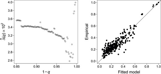
Left: The squared error defined in (23) between empirical extremal correlations and those implied by the tree metric structure for different values of the exceedance probability . Right: Extremal correlations for the spot foreign exchange rate data implied by the fitted Hüsler–Reiss tree model against the empirical counterparts
![Minimum spanning tree T^Γ of extremal dependence for the spot foreign exchange rate data based on the combined extremal variogram. The width of each edge (i,j)∈ÊΓ is proportional to the extremal correlation 2−2Φ(Γ^ij/2), and therefore wider edges indicate stronger extremal dependence. [Colour figure can be viewed at https://dbpia.nl.go.kr]](https://oup.silverchair-cdn.com/oup/backfile/Content_public/Journal/jrsssb/84/5/10.1111_rssb.12556/1/m_rssb_84_5_2055_fig-9.jpeg?Expires=1750325314&Signature=wuBYRrNnKrSHcowHr27OeZmHZ-yWBQupvjvu~FXc4e6iXOzUJifpMFQ3Pi50fEVRt7rC3WXfsQKsn-z9asmSyUa1BIl3PSPxegV4TwR0Tl33XUK7EEAN2ZmglJ-ErvCy-4CBzL5ExaVyUn5s9BwTTrBqpU0QpKOSZAeWrlXve2Mu0B8Q4vUZxfFYW50Hgxb9aQZOaycI1SCKr3lw3S7UZAwg92OGWbyrHWfJ4MmlaUJKSCMfT0qY9fG3wF606XaowoVfRn-lg-82Abo1lSfdnr6zamHAeVf0eFBFS34A5KsPfiOAyeq5JVtNNT5chkgWdcM7NhLgnnvRJ38UAbs-Nw__&Key-Pair-Id=APKAIE5G5CRDK6RD3PGA)
Minimum spanning tree of extremal dependence for the spot foreign exchange rate data based on the combined extremal variogram. The width of each edge is proportional to the extremal correlation , and therefore wider edges indicate stronger extremal dependence. [Colour figure can be viewed at https://dbpia.nl.go.kr]
The structure of the tree allows for a nice interpretation of extremal dependence. Extreme observations in the exchange rates with the Euro are strongly connected with extremes of other European currencies in Northern and Eastern countries. The graph suggests that extremes of exchange rates of these currencies are conditionally independent of exchange rates of other countries, given the value of Euro exchange rate. The Malaysian ringgit, the Chinese yuan, the Hong Kong dollar and the Taiwan dollar are strongly pegged to the US dollar and their closeness in the tree is therefore not surprising. Another branch of the tree contains several currencies of the Commonwealth. Finally, the connection between Japan and Switzerland is plausible because both currencies can be considered safe-haven currencies, which are both popular investments in times of crises.
In order to address the stability of the tree structure we bootstrap our data times and fit each time the tree structure. For generating each bootstrap sample, we draw with replacement data from the sample of filtered observations . This is a heuristic approach to assess the overall stability of our empirical conclusions to small perturbations in the data and does not have a formal theoretical justification at this point. Figure 10 shows that graph where the width of each edge is proportional to the number of times it has been selected in an extremal tree. Overall, the tree seems to be fairly stable since there is only a small number of dominant edges. Moreover, we can identify clear clusters that are connected in most of the trees, such as the European currencies. On the other hand some currencies such as the Russian ruble that do not have a dominant connection to any of these clusters. In future research, it could therefore be interesting to study structure estimation for forests, which allow to have unconnected graphs whose connected components are trees (Liu et al., 2011).
![Graph where the width of each edge is proportional to the number of times it has been selected in an extremal tree in the bootstrap procedure. [Colour figure can be viewed at https://dbpia.nl.go.kr]](https://oup.silverchair-cdn.com/oup/backfile/Content_public/Journal/jrsssb/84/5/10.1111_rssb.12556/1/m_rssb_84_5_2055_fig-10.jpeg?Expires=1750325314&Signature=yW7ZKQII49n6WNIP0HY62sSiqQfhHpMqh6ruseidOYaVKfT1L6WlH7AUooU0JjXipKVKa97b~dFh1qzGsfWfzzkga9oUxCkL~hd3bgOpapVoP~O1vANKH8OBuj2~uhj4G6wJy2BU~8K3xbeRdTbBSDUOduSy5vZNN5LVqjeiCw8rj~QNGpSJB9RuEHKpbVXVYosN9lTvzoSaaGDFWIgfBnNsLMY3-rccA0okvz8di10uJHQdJlaonI9tOOinJHKxRwzhsdQJcF4mGX2WMTeST2fOczpVIQqc2C0HopTpwtYUtiCMq~xv3-K7fEV085mJ~j2fvme22NmfhvP2fgNGdQ__&Key-Pair-Id=APKAIE5G5CRDK6RD3PGA)
Graph where the width of each edge is proportional to the number of times it has been selected in an extremal tree in the bootstrap procedure. [Colour figure can be viewed at https://dbpia.nl.go.kr]
So far we have not assumed any specific model for the extremal dependence on the edges since we are able to estimate the tree structure fully non-parametrically with the methods from this paper. If we were only interested in interpretation of the extremal graphical structure we could stop our analysis here. If we require a model for rare event simulation or risk assessment, in a second step we can choose arbitrary bivariate Pareto models for each edge. For simplicity, we choose here for all edges the Hüsler–Reiss model (see Example 4) resulting in a Hüsler–Reiss tree. For this model, the bivariate parameter estimates can be chosen directly as the empirical extremal variogram estimates for all . Alternatively, we could estimate them by censored maximum likelihood. In both cases, the remaining entries of the Hüsler–Reiss parameter matrix can be obtained from the additivity of the extremal variogram on the tree in (14). We denote the corresponding parameter matrix completed on the tree by . Recall the relation between and for Hüsler–Reiss models from Example 4. The right panel of Figure 8 shows the extremal correlations implied by the fitted Hüsler–Reiss tree model, that is, , against the empirical counterparts , . Even though the tree structure is a very sparse graph with only edges, the extremal dependence between all variables is well-explained.
DATA AVAILABILITY STATEMENT
The data that support the findings of this study are openly available in extremal_tree_learning at https://github.com/sebastian-engelke/.
ACKNOWLEDGEMENTS
The authors would like to thank Jiaying Gu for pointing us to Hall's marriage theorem, and Johan Segers for pointing us to a mistake in an earlier version of Proposition 5. We further thank Nicola Gnecco, Adrien S. Hitz, Michaël Lalancette and Chen Zhou for helpful comments. We also thank the Associate Editor and two anonymous Referees for comments which helped us to improve the presentation and for encouraging us to consider results in growing dimensions. Sebastian Engelke was supported by an Eccellenza grant of the Swiss National Science Foundation and Stanislav Volgushev was partially supported by a discovery grant from NSERC of Canada.
REFERENCES
APPENDIX
A.1 Country codes used in the application in Section 6 Country codes used in the application in Section 6
Table A1 shows the three-letter country codes of the exchange rates into British Pound sterling.
Three-letter country codes
| Code | Foreign exchange rate (into GBP) | Code | Foreign exchange rate (into GBP) |
|---|---|---|---|
| AUS | Australian Dollar | NOR | Norwegian Krone |
| CAN | Canadian Dollar | POL | Polish Zloty |
| CHN | Chinese Yuan | RUS | Russian Ruble |
| CZE | Czech Koruna | SAU | Saudi Riyal |
| DNK | Danish Krone | SGP | Singapore Dollar |
| EUR | Euro | ZAF | South African Rand |
| a HKG | Hong Kong Dollar | KOR | South Korean Won |
| HUN | Hungarian | SWE | Swedish Krona |
| IND | Indian Rupee | CHE | Swiss Franc |
| ISR | Israeli Shekel | TWN | Taiwan Dollar |
| JPN | Japanese Yen | THA | Thai Baht |
| MYS | Malaysian ringgit | TUR | Turkish Lira |
| NZL | New Zealand Dollar | USA | US Dollar |
A.2 Proof of Proposition 4
In order to show that the extremal variogram defines a tree metric on , we recall the stochastic representation of in Proposition 1. We compute
where for two sets and , denotes the symmetric difference. The second to last equality follows from the independence of the . Moreover, for the last equation we note that for two neighbouring nodes in the directed tree , by applying the same argument as above, we have .
A.3 Proof of Corollary 1
We have to show that for any tree that differs from in at least one edge, it holds
The terms for cancel directly between the two sums. For , the graph is disconnected with connected components, say, . Since is connected, there must be a and such that . Since the path must contain the edge and
this means that the first sum in (A1) contains as part of , which cancels the corresponding term in the second sum.
There are the same number of edges in as in and every for is the sum of several terms in the decomposition (A2). Therefore, the difference on the left-hand side of (A1) is indeed strictly positive as long as none of the distances vanishes.
A.4 Proof of Corollary 2
For the true edge set we observe
where the first inequality follows from the uniqueness of the minimum spanning tree with weights , . It follows that must be the minimum spanning tree corresponding to the weights .
A.5 Proof of Proposition 5
We begin by proving (15). To this end, note that we can write the extremal correlation in the extremal tree model as
From (8) we have that
and therefore, by independence between and and since follows a standard Pareto distribution,
by changing the order of integration. Observe that for any two positive, independent random variables and with , we have from Jensen's inequality by concavity of
Recall that we have for all . Since we can apply the above successively to obtain
Thus (15) follows.
We show that the minimal spanning tree is unique provided that the inequality in (15) is strict. We have to show that for any tree that differs from in at least one edge, it holds
where we let .
We will now compare the summands in the two sums in (A4) in a pairwise fashion. To this end, we will construct a bijective mapping such that for any , the corresponding edge satisfies .
Consider the undirected graph where is connected to if and only if . In this formulation, our goal is to find an -saturating matching, that is, a matching such that every element of is assigned one element in . A graphical illustration of this idea is provided in Figure A1.
![Left and center: two trees T and T′. Right: bipartite graph between elements in E and E′. A link from (i,j)∈E to (h,l)∈E′ means that (i,j)∈ph(hl;T). The blue links indicate one possible matching τ:E→E′ in this case. [Colour figure can be viewed at https://dbpia.nl.go.kr]](https://oup.silverchair-cdn.com/oup/backfile/Content_public/Journal/jrsssb/84/5/10.1111_rssb.12556/1/m_rssb_84_5_2055_fig-11.jpeg?Expires=1750325314&Signature=hSHot~tcIDo2BHmbJM2SvRc2nzG444RBpgYEEu9taQoyF6j9AQE-5Kf8zJj7BA76x34WuNszqepoVG06fkaN0JuuQKpfvGZTVxejle88AZyKOda9UAi6PRBj-Aj7yBvCyODv0arfbWXqctN64BzNi9ZrZ6mahp~DYzWyLIgkByAAk-JWOMx49MsGAJ2Y4IasK1HKCijuF9Wx6ndXuZxLgZOeh4fRx6~yizl7Rge9EIx~xArGsizxNo-5DdEaEbIYgrYOPQDb8J619Hp75TZBN4Rn8kqZYBjMQTDtL--KRPJ4XxsqiGWtPX41MqLXykOR-J9Lo3fffdHPz-BEiNO97g__&Key-Pair-Id=APKAIE5G5CRDK6RD3PGA)
Left and center: two trees and . Right: bipartite graph between elements in and . A link from to means that . The blue links indicate one possible matching in this case. [Colour figure can be viewed at https://dbpia.nl.go.kr]
By Hall's marriage theorem (Hall, 1935), such a matching exists provided that for any subset , the corresponding neighbourhood of elements in that are connected to at least one of the elements in satisfies
Let be the edges in , where . Removing these edges from the tree results in a graph with connected components, which we denote by .
Starting with component , we know from the connectedness of the tree that there must be an edge in between at least one of the elements of , say , to for some . Since and are in different connected components in , the path must contain one of the edges in , and therefore .
Similarly, there must exist an edge between an element and some , . This edge is necessarily different from as it has a node in , and the path must contain one of the edges in because are in different connected components of . Thus .
Continuing this argument inductively we obtain different edges in and therefore the condition (A5) holds.
In order to show inequality (A4) we rewrite the left-hand side as
By construction of , for , the path must contain the edge and thus by (15)
This means that all summands in (A6) are non-negative. Recall that we assume in the second part of Proposition 5 that the inequalities (15) are strict for . Since there is at least one , the first inequality in (A7) is strict for this edge and therefore, the difference on the left-hand side of (A4) is indeed strictly positive. Thus the proof is complete.
Author notes
Funding information Natural Sciences and Engineering Research Council of Canada, Schweizerischer Nationalfonds zur Förderung der Wissenschaftlichen Forschung, Grant/Award Number: 161297
