


Abstract
We study the problem of high-dimensional Principal Component Analysis (PCA) with missing observations. In a simple, homogeneous observation model, we show that an existing observed-proportion weighted (OPW) estimator of the leading principal components can (nearly) attain the minimax optimal rate of convergence, which exhibits an interesting phase transition. However, deeper investigation reveals that, particularly in more realistic settings where the observation probabilities are heterogeneous, the empirical performance of the OPW estimator can be unsatisfactory; moreover, in the noiseless case, it fails to provide exact recovery of the principal components. Our main contribution, then, is to introduce a new method, which we call primePCA, that is designed to cope with situations where observations may be missing in a heterogeneous manner. Starting from the OPW estimator, primePCA iteratively projects the observed entries of the data matrix onto the column space of our current estimate to impute the missing entries, and then updates our estimate by computing the leading right singular space of the imputed data matrix. We prove that the error of primePCA converges to zero at a geometric rate in the noiseless case, and when the signal strength is not too small. An important feature of our theoretical guarantees is that they depend on average, as opposed to worst-case, properties of the missingness mechanism. Our numerical studies on both simulated and real data reveal that primePCA exhibits very encouraging performance across a wide range of scenarios, including settings where the data are not Missing Completely At Random.
1 INTRODUCTION
One of the ironies of working with Big Data is that missing data play an ever more significant role, and often present serious difficulties for analysis. For instance, a common approach to handling missing data is to perform a so-called complete-case analysis (Little & Rubin, 2019), where we restrict attention to individuals in our study with no missing attributes. When relatively few features are recorded for each individual, one can frequently expect a sufficiently large proportion of complete cases that, under an appropriate missing at random (MAR) hypothesis, a complete-case analysis may result in only a relatively small loss of efficiency. On the other hand, in high-dimensional regimes where there are many features of interest, there is often such a small proportion of complete cases that this approach becomes infeasible. As a very simple illustration of this phenomenon, imagine an data matrix in which each entry is missing independently with probability 0.01. When , a complete-case analysis would result in around 95 of the individuals (rows) being retained, but even when we reach , only around 5 of rows will have no missing entries.
The inadequacy of the complete-case approach in many applications has motivated numerous methodological developments in the field of missing data over the past 60 years or so, including imputation (Ford, 1983; Rubin, 2004), factored likelihood (Anderson, 1957) and maximum likelihood approaches (Dempster et al., 1977); see, for example, Little & Rubin (2019) for an introduction to the area. Recent years have also witnessed increasing emphasis on understanding the performance of methods for dealing with missing data in a variety of high-dimensional problems, including sparse regression (Belloni et al., 2017; Loh & Wainwright, 2012), classification (Cai & Zhang, 2018), sparse principal component analysis (Elsener & van de Geer, 2018) and covariance and precision matrix estimation (Loh & Tan, 2018; Lounici, 2014).
In this paper, we study the effects of missing data in one of the canonical problems of high-dimensional data analysis, namely dimension reduction via Principal Component Analysis (PCA). This is closely related to the topic of matrix completion, which has received a great deal of attention in the literature over the last decade or so (Candès et al., 2011; Candès & Plan, 2010; Candès & Recht, 2009; Keshavan et al., 2010; Koltchinskii et al., 2011; Mazumder et al., 2010; Negahban & Wainwright, 2012) for example. There, the focus is typically on accurate recovery of the missing entries, subject to a low-rank assumption on the signal matrix; by contrast, our focus is on estimation of the principal eigenspaces. Previously proposed methods for low-dimensional PCA with missing data include non-linear iterative partial least squares (Wold & Lyttkens, 1969), iterative PCA (Josse & Husson, 2012; Kiers, 1997) and its regularised variant (Josse et al., 2009); see Dray & Josse (2015) for a nice survey and comparative study. More broadly, the R-miss-tastic website https://rmisstastic.netlify.com/ provides a valuable resource on methods for handling missing data.
The importance of the problem of high-dimensional PCA with missing data derives from its wide variety of applications. For instance, in many commercial settings, one may have a matrix of customers and products, with entries recording the number of purchases. Naturally, there will typically be a high proportion of missing entries. Nevertheless, PCA can be used to identify items that distinguish the preferences of customers particularly effectively, to make recommendations to users of products they might like and to summarise efficiently customers' preferences. Later, we will illustrate such an application, on the Million Song Dataset, where we are able to identify particular songs that have substantial discriminatory power for users' preferences as well as other interesting characteristics of the user database. Other potential application areas include health data, where one may seek features that best capture the variation in a population, and where the corresponding principal component scores may be used to cluster individuals into subgroups (that may, for instance, receive different treatment regimens).
To formalise the problem we consider, suppose that the (partially observed) matrix matrix is of the form
for independent random matrices and , where is a low-rank matrix and is a noise matrix with independent and identically distributed entries having zero mean. The low-rank property of is encoded through the assumption that it is generated via
where has orthonormal columns and is a random matrix (with ) having independent and identically distributed rows with mean zero and covariance matrix . Note that when and are independent, the covariance matrix of has a -spiked structure; such covariance models have been studied extensively in both theory and applications (Cai et al., 2013; Fan et al., 2013; Johnstone & Lu, 2009; Paul, 2007).
We are interested in estimating the column space of , denoted by , which is also the -dimensional leading eigenspace of . Cho et al. (2017) considered a different but related model where in (2) is deterministic, and is not necessarily centred, so that is the top right singular space of . (By contrast, in our setting, , so the mean structure is uninformative for recovering .) Their model can be viewed as being obtained from the model (1) and (2) by conditioning on . In the context of a -homogeneous Missing Completely At Random (MCAR) observation model, where each entry of is observed independently with probability (independently of , Cho et al. (2017) studied the estimation of by , where is a simple estimator formed as the top eigenvectors of an observed-proportion weighted (OPW) version of the sample covariance matrix (here, the weighting is designed to achieve approximate unbiasedness). Our first contribution, in Section 2, is to provide a detailed, finite-sample analysis of this estimator in the model given by (1) and (2) together with a -homogeneous MCAR missingness structure, with a noise level of constant order. The differences between the settings necessitate completely different arguments, and reveal in particular a new phenomenon in the form of a phase transition in the attainable risk bound for the loss function, that is, the Frobenius norm of the diagonal matrix of the sines of the principal angles between and . Moreover, we also provide a minimax lower bound in the case of estimating a single principal component, which reveals that this estimator achieves the minimax optimal rate up to a poly-logarithmic factor.
While this appears to be a very encouraging story for the OPW estimator, it turns out that it is really only the starting point for a more complete understanding of high-dimensional PCA with missing data. For instance, in the noiseless case, the OPW estimator fails to provide exact recovery of the principal components. Moreover, it is the norm rather than the exception in applications that missingness is heterogeneous, in the sense that the probability of observing entries of varies (often significantly) across columns. For instance, in recommendation systems, some products will typically be more popular than others, and hence we observe more ratings in those columns. As another example, in meta-analyses of data from several studies, it is frequently the case that some covariates are common across all studies, while others appear only in a reduced proportion of them. In Section 2.2, we present an example to show that, even with an MCAR structure, PCA algorithms can break down entirely for such heterogeneous observation mechanisms when individual rows of can have large Euclidean norm. Intuitively, if we do not observe the interaction between the th and th columns of , then we cannot hope to estimate the th or th rows of , and this will cause substantial error if these rows of contain significant signal. This example illustrates that it is only possible to handle heterogeneous missingness in high-dimensional PCA with additional structure, and indicates that it is natural to measure the difficulty of the problem in terms of the incoherence among the entries of —that is, the maximum Euclidean norm of the rows of .
Our main contribution, then, is to propose a new, iterative algorithm, called primePCA (short for projected refinement for imputation of missing entries in Principal Component Analysis), in Section 3, to estimate , even with heterogeneous missingness. The main initialiser that we study for this algorithm is a modified version of the simple estimator discussed above, where the modification accounts for potential heterogeneity. Each iteration of primePCA projects the observed entries of onto the column space of the current estimate of to impute missing entries, and then updates our estimate of by computing the leading right singular space of the imputed data matrix. An illustration of the two steps of a single iteration of the primePCA algorithm in the case , is given in Figure 1.
![An illustration of the two steps of a single iteration of the primePCA algorithm with d=3 and K=1. Black dots represent fully observed data points, while vertical dotted lines that emanate from them give an indication of their x3 coordinate values, as well as their projections onto the x1-x2 plane. The x1 coordinate of the orange data point and the x2 coordinate of the blue data point are unobserved, so the true observations lie on the respective solid lines through those points (which are parallel to the relevant axes). Starting from an input estimate of VK (left), given by the black arrow, we impute the missing coordinates as the closest points on the coloured lines to VK (middle), and then obtain an updated estimate of VK as the leading right singular vector of the imputed data matrix (right, with the old estimate in grey). [Colour figure can be viewed at https://dbpia.nl.go.kr]](https://oup.silverchair-cdn.com/oup/backfile/Content_public/Journal/jrsssb/84/5/10.1111_rssb.12550/1/m_rssb_84_5_2000_fig-1.jpeg?Expires=1750218786&Signature=mdI9SO-Bkq1h8nOe8eeAyGhUWH7oShqGjI7pnpAiYDKhAitBNnyK8l2J2nPiQU3GalLOzhaI0EIwoDn6ezqkkCiGif1Sz7OjdVcxq2amxhtfJKJ1bSOA-PVWcKMlsWoEh4c1cw2LyuFtAISeNEBU7uose5SKAlwXgrJ2OkAcJt1cpSu0H1k4pZWJCmNDQ-xG7GJTecpFumCLFTira216dKyMecvhQjb7ivhIyVQgg1VqA0eR4XCNWa57zwCZRdRou06Yommo0Dn96c2kXkxk1hT3Wsbjw7NxtWvt5xr549p-OfssLZwqjcm8O-p3nGt3yTfN6ewMYt3aBfDlyPZh8g__&Key-Pair-Id=APKAIE5G5CRDK6RD3PGA)
An illustration of the two steps of a single iteration of the primePCA algorithm with and . Black dots represent fully observed data points, while vertical dotted lines that emanate from them give an indication of their coordinate values, as well as their projections onto the - plane. The coordinate of the orange data point and the coordinate of the blue data point are unobserved, so the true observations lie on the respective solid lines through those points (which are parallel to the relevant axes). Starting from an input estimate of (left), given by the black arrow, we impute the missing coordinates as the closest points on the coloured lines to (middle), and then obtain an updated estimate of as the leading right singular vector of the imputed data matrix (right, with the old estimate in grey). [Colour figure can be viewed at https://dbpia.nl.go.kr]
Our theoretical results reveal that in the noiseless setting, that is, , primePCA achieves exact recovery of the principal eigenspaces (with a geometric convergence rate) when the initial estimator is close to the truth and a sufficiently large proportion of the data are observed. Moreover, we also provide a performance guarantee for the initial estimator, showing that under appropriate conditions it satisfies the desired requirement with high probability, conditional on the observed missingness pattern. Code for our algorithm is available in the R package primePCA (Zhu et al., 2019).
To the best of our knowledge, primePCA is the first method for high-dimensional PCA that is designed to cope with settings where missingness is heterogeneous. Indeed, the previously mentioned works on high-dimensional PCA and other high-dimensional statistical problems with missing data have either focused on a uniform missingness setting or have imposed a lower bound on entrywise observation probabilities, which reduces to this uniform case. In particular, such results fail to distinguish in terms of the performance of their algorithms between a setting where one variable is observed with a very low probability and all other variables are fully observed, and a setting where all variables are observed with probability . A key contribution of our work is to account explicitly for the effect of a heterogeneous missingness mechanism, where the estimation error depends on average entrywise missingness rather than worst-case missingness; see the discussions after Theorem 4 and Proposition 2 below. In Section 4, the empirical performance of primePCA is compared with both that of the initialiser, and a popular method for matrix completion called softImpute (Hastie et al., 2015; Mazumder et al., 2010); we also discuss maximum likelihood approaches implemented via the Expectation–Maximisation (EM) algorithm, which can be used when the dimension is not too high. Our settings include a wide range of signal-to-noise ratios (SNRs), as well as Missing Completely At Random, MAR and Missing Not At Random (MNAR) examples (Little & Rubin, 2019; Seaman et al., 2013). These comparisons reveal that primePCA provides highly accurate and robust estimation of principal components, for instance outperforming the softImpute algorithm, even when the latter is allowed access to the oracle choice of regularisation parameter for each dataset. Our analysis of the Million Song Dataset is given in Section 5. In Section 6, we illustrate how some of the ideas in this work may be applied to other high-dimensional statistical problems involving missing data. Proofs of our main results are deferred to Section A in Appendix S1 (Zhu et al., 2019); auxiliary results and their proofs are given in Section B of Appendix S1.
1.1 Notation
For a positive integer , we write . For and , we define and . We let denote the unit Euclidean sphere in .
Given , we write for the diagonal matrix whose th diagonal entry is . We let denote the set of matrices in with orthonormal columns. For a matrix , and , we write if and for its entrywise norm, as well as for its -to- operator norm. We provide special notation for the (Euclidean) operator norm and the Frobenius norm by writing and respectively. We also write for the th largest singular value of , and define its nuclear norm by . If , we write for the matrix obtained by extracting the rows of that are in . For , the Hadamard product of and , denoted , is defined such that for any and .
2 THE OPW ESTIMATOR
In this section, we study a simple OPW estimator of the matrix of principal components. To define the estimator, let denote the event that the th entry of is observed. We define the revelation matrix by , and the partially observed data matrix
Our observed data are the pair (). Importantly, the fact that we observe allows us to distinguish between observed zeros and missing entries (even though these also appear as zeros in ). We first consider the simplest possible case, which we refer to as the -homogeneous observation model, where entries of the data matrix are observed independently and completely at random (i.e., independent of ), each with probability . Thus, for all , and and are independent for .
For , let and denote the th rows of and , respectively, and define . Writing and for its entrywise inverse, we have that under the -homogeneous observation model, and . Following Lounici (2013, 2014) and Cho et al. (2017), we consider the following weighted sample covariance matrix:
The reason for including the weight is to ensure that , so that is an unbiased estimator of . Related ideas appear in the work of Cai & Zhang (2016) on high-dimensional covariance matrix estimation with missing data; see also Little & Rubin (2019, section 3.4). In practice, is typically unknown and needs to be estimated. It is therefore natural to consider the following plug-in estimator :
where and denotes the proportion of observed entries in . The OPW estimator of , denoted , is the matrix formed from the top eigenvectors of .
2.1 Theory for homogeneous missingness
We begin by studying the theoretical performance of in a simple model that will allow us to reveal an interesting phase transition for the problem. For a random vector taking values in and for , we define its (Orlicz) -norm and a version that is invariant to invertible affine transformations by
respectively. Recall that we say is sub-Gaussian if .
In this preliminary section, we assume that is generated according to (1), (2) and (3), where:
- (A1)
, and are independent;
- (A2)
has independent and identically distributed rows with and ;
- (A3)
has independent and identically distributed entries with , and ;
- (A4)
for all ;
- (A5)
has independent entries.
Thus, (A1) ensures that the complete data matrix and the revelation matrix are independent; in other words, for now we work in a Missing Completely At Random (MCAR) setting. In a homoscedastic noise model, there is no loss of generality (by a scaling argument) in assuming that each entry of has unit variance, as in (A3). In many places in this work, it will be convenient to think intuitively of and in (A2)–(A4) as constants. In particular, if has multivariate normal rows and has normal entries, then we can simply take . For , under the same normality assumptions, we have , so this intuition amounts to thinking of the variance of each component of our data as being of constant order.
A natural measure of the performance of an estimator of is given by the Davis–Kahan loss
(Davis & Kahan, 1970)1. Our first theorem controls the risk of the OPW estimator; here and below, we write for the th largest eigenvalue of .
Theorem 1Assume (A1)–(A5) and that, . Write. Then there exists a universal constantsuch that
(5)In particular, if, then there exists, depending only onand, such that
(6)
Theorem 1 reveals an interesting phase transition phenomenon. Specifically, if the signal strength is large enough that , then we should regard as the effective sample size, as might intuitively be expected. On the other hand, if , then the estimation problem is considerably more difficult and the effective sample size is of order . In fact, by inspecting the proof of Theorem 1, we see that in the high signal case, it is the difficulty of estimating the diagonal entries of that drives the rate, while when the signal strength is low, the bottleneck is the challenge of estimating the off-diagonal entries. By comparing (6) with the minimax lower bound result in Theorem 2 below, we see that this phase transition phenomenon is an inherent feature of this estimation problem, rather than an artefact of the proof techniques we used to derived the upper bound.
The condition in Theorem 1 is reasonable given the scaling requirement for consistency of the empirical eigenvectors (Johnstone & Lu, 2009; Shen et al., 2016; Wang & Fan, 2017). Indeed, Shen et al. (2016, Theorem 5.1) show that when , the top eigenvector of the sample covariance matrix estimator is consistent if and only if . If we regard as the effective sample size in our missing data PCA problem, then it is a sensible analogy to assume that here, which implies that the condition holds for large , up to poly-logarithmic factors.
As mentioned in the introduction, Cho et al. (2017) considered the different but related problem of singular space estimation in a model in which , where is a matrix of the form for a deterministic matrix , whose rows are not necessarily centred. In this setting, is the matrix of top right singular vectors of , and the same estimator can be applied. An important distinction is that, when the rows of are not centred and the entries of are of comparable magnitude, is of order , so when is regarded as a constant, it is natural to think of the singular values of as also being of order . Indeed, this is assumed in Cho et al. (2017). On the other hand, in our model, where the rows of have mean zero, assuming that the eigenvalues are of order would amount to an extremely strong requirement, essentially restricting attention to very highly spiked covariance matrices. Removing this condition in Theorem 1 requires completely different arguments.
In order to state our minimax lower bound, we let denote the class of distributions of pairs satisfying (A1), (A2), (A3) and (A5) with . Since we are now working with vectors instead of matrices, we write in place of .
Theorem 2There exists a universal constantsuch that
where the infimum is taken over all estimatorsof.
Theorem 2 reveals that in Theorem 1 achieves the minimax optimal rate of estimation up to a poly-logarithmic factor when and are regarded as constants.
2.2 Heterogeneous observation mechanism
A key assumption of the theory in Section 2.1, which allowed even a very simple estimator to perform well, was that the missingness probability was homogeneous across the different entries of the matrix. On the other hand, the aim of this sub-section is to show that the situation changes dramatically once the data can be missing heterogeneously.
To this end, consider the following example. Suppose that is equal to or with equal probability, so that
In other words, for each , we observe precisely one of the first two entries of , together with all of the remaining entries. Let , where , and , where . Suppose that and let , and similarly assume that and set . Then and are identically distributed. However, the leading eigenvectors of and are respectively and , which are orthogonal!
Thus, it is impossible to simultaneously estimate consistently the leading eigenvector of both and from our observations. We note that it is the disproportionate weight of the first two coordinates in the leading eigenvector, combined with the failure to observe simultaneously the first two entries in the data, that makes the estimation problem intractable in this example. The understanding derived from this example motivates us to seek bounds on the error in high-dimensional PCA that depend on an incoherence parameter . The intuition here is that the maximally incoherent case is where each column of is a unit vector proportional to a vector whose entries are either 1 or , in which case and . On the other hand, in the worst case, when the columns of are the first standard basis vectors in , we have . Bounds involving incoherence have appeared previously in the literature on matrix completion (e.g., Candès & Plan, 2010; Keshavan et al., 2010), but for a different reason. There, the purpose is to control the principal angles between the true right singular space and the standard basis, which yields bounds on the number of observations required to infer the missing entries of the matrix. In our case, the incoherence condition controls the extent to which the loadings of the principal components of interest are concentrated in any single coordinate, and therefore the extent to which significant estimation error in a few components of the leading eigenvectors can affect the overall statistical performance. In the intractable example above, , and with such a large value of , heavy corruption from missingness in only a few entries spoils any chance of consistent estimation.
3 OUR NEW ALGORITHM FOR PCA WITH MISSING ENTRIES
We are now in a position to introduce and analyse our iterative algorithm primePCA to estimate , the principal eigenspace of the covariance matrix . The basic idea is to iterate between imputing the missing entries of the data matrix using a current (input) iterate , and then applying a singular value decomposition (SVD) to the completed data matrix. More precisely, for , we let denote the indices for which the corresponding entry of is observed, and regress the observed data on to obtain an estimate of the th row of . This is natural in view of the data generating mechanism . We then use to impute the missing values , retain the original observed entries as , and set our next (output) iterate to be the top right singular vectors of the imputed matrix . To motivate this final choice, observe that when , we have ; we therefore have the SVD , where and is diagonal with positive diagonal entries. This means that , so the column spaces of and coincide. For convenience, pseudocode of a single iteration of refinement in this algorithm is given in Algorithm 1.
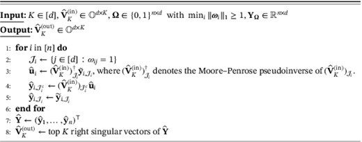
refine , a single step of refinement of current iterate
We now seek to provide formal justification for Algorithm 1. The recursive nature of the primePCA algorithm induces complex relationships between successive iterates, so to facilitate theoretical analysis, we will impose some conditions on the underlying data generating mechanism that may not hold in situations where we would like to apply to algorithm. Nevertheless, we believe that the analysis provides considerable insight into the performance of the primePCA algorithm, and these are discussed extensively below; moreover, our simulations in Section 4 consider settings both within and outside the scope of our theory, and confirm its attractive and robust numerical performance.
In addition to the loss function , it will be convenient to define a slightly different notion of distance between subspaces. For any , we let be an SVD of . The two-to-infinity distance between and is then defined to be
We remark that the definition of does not depend on our choice of SVD and that for any , so that really represents a distance between the subspaces spanned by and . In fact, there is a sense in which the change-of-basis matrix tries to align the columns of as closely as possible with those of ; more precisely, if we change the norm from the two-to-infinity operator norm to the Frobenius norm, then uniquely solves the so-called Procrustes problem (Schönemann, 1966):
The following proposition considers the noiseless setting , and shows that, for any estimator that is close to , a single iteration of refinement in Algorithm 1 contracts the two-to-infinity distance between their column spaces, under appropriate conditions. We define .
Proposition 1Letas in Algorithm1and further let. We assume thatand that. Suppose thatand that the SVD ofis of the form, whereandfor some. Then there exist, depending only on, such that whenever
- (i)
,
- (i)
,
we have that
In order to understand the main conditions of Proposition 1, it is instructive to consider the case , as was illustrated in Figure 1, and initially to think of as a constant. In that case, condition (i) asks that the absolute value of every component of the difference between the vectors and is ; for intuition, if two vectors are uniformly distributed on , then each of their norms is ; in other words, we only ask that the initialiser is very slightly better than a random guess. In Condition (ii), being less than 1 is equivalent to the proportion of missing data in each column being less than (where again depends only on , and the conclusion is that the refine step contracts the initial two-to-infinity distance from by at least a factor of . In the noiseless setting of Proposition 1, the matrix of right singular vectors of has the same column span (and hence the same two-to-infinity norm) as . We can therefore gain some intuition about the scale of by considering the situation where is uniformly distributed on , so in particular, the columns of are uniformly distributed on . By Vershynin (2018, Theorem 5.1.4), we deduce that . On the other hand, when the distribution of is invariant under left multiplication by an orthogonal matrix (e.g. if has independent and identically distributed Gaussian rows), then is distributed uniformly on . Arguing as above, we see that, with high probability, we may take . This calculation suggests that we do not lose too much by thinking of as a constant (or at most, growing very slowly with and ).
To apply Proposition 1, we also require conditions on and . In practice, if either of these conditions is not satisfied, we first perform a screening step that restricts attention to a set of row indices for which the data contain sufficient information to estimate the principal components. This screening step is explicitly accounted for in Algorithm 2, as well as in the theory that justifies it. An alternative would be to seek to weight rows according to their utility for principal component estimation, but it seems difficult to implement this in a principled way that facilitates formal justification.
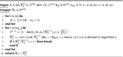
primePCA, an iterative algorithm for estimating VK given initialiser
Algorithm 2 provides pseudocode for the iterative primePCA algorithm, given an initial estimator . The iterations continue until either we hit the convergence threshold or the maximum iteration number . Theorem 3 below guarantees that, in the noiseless setting of Proposition 1, the primePCA estimator converges to at a geometric rate.
Theorem 3For, letbe theiterate of Algorithm2with input, , , , , and. Write, and let
where. Suppose thatand that the SVD ofis of the form, whereandfor some. Assume that
Then there exist, depending only and , such that whenever
- (i)
,
- (ii)
,
we have that for every,
The condition that amounts to the very mild assumption that the algorithmic input is not exactly equal to any element of the set , though the conditions on and become milder as increases.
3.1 Initialisation
Theorem 3 provides a general guarantee on the performance of primePCA, but relies on finding an initial estimator that is sufficiently close to the truth . The aim of this sub-section, then, is to propose a simple initialiser and show that it satisfies the requirement of Theorem 3 with high probability, conditional on the missingness pattern.
Consider the following modified weighted sample covariance matrix
where for any ,
Here, the matrix replaces in (4) because, unlike in Section 2.1, we no longer wish to assume homogeneous missingness. We take as our initial estimator of the matrix of top eigenvectors of , denoted . Theorem 4 below studies the performance of this initialiser, in terms of its two-to-infinity norm error, and provides sufficient conditions for us to be able to apply Theorem 3. In particular, it ensures that the initialiser is reasonably well-aligned with the target . We write and for probabilities and expectations conditional on .
Theorem 4Assume (A1)–(A4) and that. Suppose further that, that for alland let. Then there exist, depending only onand, such that for every, if
(10)then
As a consequence, writing
where and are as in Theorem3, we have that
The first part of Theorem 4 provides a general probabilistic upper bound for , after conditioning on the missingness pattern. This allows us, in the second part, to provide a guarantee on the probability with which is a good enough initialiser for Theorem 3 to apply. For intuition regarding , consider the MCAR setting with for . In that case, by Lemma 6, typical realisations of have and when is small. In particular, when , we expect to be small when and are both of the same order, and grow faster than
As a special case, in the -homogeneous model where for , the requirement on above is that it should grow faster than .
One of the attractions of our analysis is the fact that we are able to provide bounds that only depend on entrywise missingness probabilities in an average sense, as opposed to worst-case missingness probabilities. The refinements conferred by such bounds are particularly important when the missingness mechanism is heterogeneous, as typically encountered in practice. The averaging of missingness probabilities can be partially seen in Theorem 4, since and depend only on the and norms of each row of , but is even more evident in the proposition below, which gives a probabilistic bound on the original distance between and .
Proposition 2Assume the same conditions as in Theorem4. Then there exists a universal constantsuch that for any, if
(11)then
In this bound, we see that only depends on through the entrywise and norms of the whole matrix. Lemma 6 again provides probabilistic control of these norms under the -homogeneous missingness mechanism. In general, if the rows of are independent and identically distributed, but different covariates are missing with different probabilities, then off-diagonal entries of will concentrate around the reciprocals of the simultaneous observation probabilities of pairs of covariates. As such, for a typical realisation of , our bound in Proposition 2 depends only on the harmonic averages of these simultaneous observation probabilities and their squares. Such an averaging effect ensures that our method is effective in a much wider range of heterogeneous settings than previously allowed in the literature.
3.2 Weakening the missingness proposition condition for contraction
Theorem 3 provides a geometric contraction guarantee for the primePCA algorithm in the noiseless case. The price we pay for this strong conclusion, however, is a strong condition on the proportion of missingness that enters the contraction rate parameter through ; indeed in an asymptotic framework where the incoherence parameter grows with the sample size and/or dimension, the proportion of missingness would need to vanish asymptotically. Therefore, to complement our earlier theory, we present below Proposition 3 and Corollary 1. Proposition 3 is an analogue of the deterministic Proposition 1 in that it demonstrates that a single iteration of the primePCA algorithm yields a contraction provided that the input is sufficiently close to . The two main differences are first that the contraction is in terms of a Procrustes-type loss (see the discussion around (7)), which turns out to be convenient for Corollary 1; and second, the bound depends only on the incoherence of the matrix , and not on the corresponding quantity for .
Proposition 3Let, letand let. Fix and with, and let, with. Suppose thatare such that for every,
(12)Assume further that
(13)Then the outputof Algorithm1satisfies
where.
Interestingly, the proof of Proposition 3 proceeds in a very different fashion from that of Proposition 1. The key step is to bound the discrepancy between the principal components of the imputed data matrix in Algorithm 1 and using a modified version of Wedin's theorem (Wang, 2016). To achieve the desired contraction rate, instead of viewing the true data matrix as the reference matrix when calculating the perturbation, we choose a different reference matrix with the same top right singular space as but which is closer to in terms of the Frobenius norm. Such a reference shift sharpens the eigenspace perturbation bound.
The contraction rate in Proposition 3 is a sum of three terms, the first two of which are small provided that is small and is large respectively. On the other hand, the final term is small provided that no small subset of the rows of contributes excessively to its operator norm. For different missingness mechanisms, such a guarantee would need to be established probabilistically on a case-by-case basis; in Corollary 1 we illustrate how this can be done to achieve a high probability contraction in the simplest missingness model. Importantly, the proportion of missingness allowed, and hence the contraction rate parameter, no longer depend on the incoherence of , and can be of constant order.
Corollary 1Consider the-homogeneous MCAR setting. Fixandwith, and let, with. Suppose that, and are as in Proposition 3, let , and, fixing , suppose that
Suppose that. Then with probability at least, the outputof Algorithm1satisfies
To understand the conclusion of Corollary 1, it is instructive to consider the special case . Here, and is the ratio of the and norms of the vector . When the entries of this vector are of comparable magnitude, is therefore of order , so the contraction rate is of order .
3.3 Other missingness mechanisms
Another interesting aspect of our theory is that the guarantees provided in Theorem 3 are deterministic. Provided we start with a sufficiently good initialiser, Theorem 3 describes the way in which the performance of primePCA improves over iterations. An attraction of this approach is that it offers the potential to study the performance of primePCA under more general missingness mechanisms. For instance, one setting of considerable practical interest is the MAR model, which postulates that our data vector and observation indicator vector satisfy
for all and . In other words, the probability of seeing a particular missingness pattern only depends on the data vector through components of this vector that are observed. Thus, if we want to understand the performance of primePCA under different missingness mechanisms, such as specific MAR (or even MNAR) models, all we require is an analogue of Theorem 4 on the performance of the initialiser in these new missingness settings. Such results, however, are likely to be rather problem-specific in nature, and it can be that choosing an initialiser based on available information on the dependence between the observations and the missingness mechanism makes it easier to prove the desired performance guarantees.
We now provide an example to illustrate how such initialisers can be constructed and analysed. Consider an MAR setting where the missingness pattern depends on the data matrix only through a fully observed categorical variable. In this case, we can construct a variant of the OPW estimator, denoted , by modifying the weighted sample covariance matrix in (8) to condition on the fully observed covariate, and then take the leading eigenvectors of an appropriate average of these conditional weighted sample covariance matrices. Specifically, suppose that our data consist of independent and identically distributed copies of , where , where is a categorical random variable taking values in and where is independent of for all . Writing , and , we have that , that is, is block diagonal. Thus, introducing the subscript for our th observation, as a starting point to construct , it is natural to consider an oracle estimator of , given by
where . Observe that we can write
where and where is the OPW estimator of based on the observations with . Hence, is unbiased for , because
In practice, when is unknown, we can estimate it by
and substitute this estimate into to obtain empirical estimators and of and , respectively. Finally, can be obtained as the matrix of top eigenvectors of the matrix
To sketch the way to bound the loss of such an initialiser, we can condition on and apply matrix Bernstein concentration inequalities similarly to those in the proof of Theorem 1 to show that is close to for each . Simple binomial concentration bounds then allow us to combine these to control , and then apply a variant the Davis–Kahan theorem to obtain a final result.
While different initialisers can be designed and analysed theoretically in specific missingness settings, as shown in the example above, our empirical experience, nevertheless, is that regardless of the missingness mechanism, primePCA is extremely robust to the choice of initialiser. This is evident from the discussion of the performance of primePCA in MAR and MNAR settings given in Section 4.4.
4 SIMULATION STUDIES
In this section, we assess the empirical performance of primePCA, as proposed in Algorithm 2, with initialiser from Section 3.1, and denote the output of this algorithm by . In Sections 4.1, 4.2 and 4.3, we generate observations according to the model described in (1), (2) and (3) where the rows of the matrix are independent random vectors, for some positive semi-definite . We further generate the observation indicator matrix , independently of and , and investigate the following four missingness mechanisms that represent different levels of heterogeneity:
- (H1)
Homogeneous: for all ;
- (H2)
Mildly heterogeneous: for , where and independently;
- (H3)
Highly heterogeneous columns: for and all odd and for and all even .
- (H4)
Highly heterogeneous rows: for and all odd and for and all even .
In Sections 4.1, 4.2 and 4.3 below, we investigate primePCA in noiseless, noisy and misspecified settings, respectively. Section 4.4 is devoted to MAR and MNAR settings. In all cases, the average statistical error was estimated from 100 Monte Carlo repetitions of the experiment. For comparison, we also studied the softImpute algorithm (Hastie et al., 2015; Mazumder et al., 2010), which is considered to be state-of-the-art for matrix completion (Chi et al., 2018). This algorithm imputes the missing entries of by solving the following nuclear-norm-regularised optimisation problem:
where is to be chosen by the practitioner. The softImpute estimator of is then given by the matrix of top right singular vectors of . In practice, the optimisation is carried out by representing as , and performing alternating projections to update and iteratively. The fact that the softImpute algorithm was originally intended for matrix completion means that it treats the left and right singular vectors symmetrically, whereas the primePCA algorithm, which has the advantage of a clear geometric interpretation as exemplified in Figure 1, focuses on the target of inference in PCA, namely the leading right singular vectors.
Figure 2 presents Monte Carlo estimates of for different choices of in two different settings. The first uses the noiseless set-up of Section 4.1, together with missingness mechanism (H1); the second uses the noisy setting of Section 4.2 with parameter and missingness mechanism (H2). We see that the error barely changes when varies within ; very similar plots were obtained for different data generation and missingness mechanisms, though we omit these for brevity. For definiteness, we therefore fixed throughout our simulation study.

4.1 Noiseless case
In the noiseless setting, we let , and also fix , , and . We set
In Figure 3, we present the (natural) logarithm of the estimated average loss of primePCA and softImpute under (H1), (H2), (H3) and (H4). We set the range of -axis to be the same for each method to facilitate straightforward comparison. We see that the statistical error of primePCA decreases geometrically as the number of iterations increases, which confirms the conclusion of Theorem 3 in this noiseless setting. Moreover, after a moderate number of iterations, its performance is a substantial improvement on that of the softImpute algorithm, even if this latter algorithm is given access to an oracle choice of the regularisation parameter . The high statistical error of softImpute in these settings can be partly explained by the default value of the tuning parameter thresh in the softImpute package in , namely , which corresponds to the red curve in the right-hand panels of Figure 3. By reducing the values of thresh to and , corresponding to the green and blue curves in Figure 3, respectively, we were able to improve the performance of softImpute to some extent, though the statistical error is sensitive to the choice of the regularisation parameter . Moreover, even with the optimal choice of , it is not competitive with primePCA. Finally, we mention that for the 2000 iterations of setting (H2), primePCA took on average just under 10 min per repetition to compute, whereas the solution path of softImpute with took around 36 min per repetition.
![Logarithms of the average Frobenius norm sinΘ error of primePCA and softImpute under various heterogeneity levels of missingness in absence of noise. The four rows of plots above, from the top to bottom, correspond to (H1), (H2), (H3) and (H4). [Colour figure can be viewed at https://dbpia.nl.go.kr]](https://oup.silverchair-cdn.com/oup/backfile/Content_public/Journal/jrsssb/84/5/10.1111_rssb.12550/1/m_rssb_84_5_2000_fig-3.jpeg?Expires=1750218786&Signature=y7Fw5mY8MjsjbNxtGPzHeDsGTX3AHxYeKB3twMKAmUlvMMOSDW16rLb7b4MrwnVfUhBY-cwC5BVlebMKS9RuKnSEY69r-9b0bwy8s-tdm69LXQ1YrRtzRw4sHZDqPfnu9iNgxwunYkjYY5VL4blnE~j6brFcaJ2mTG3fR-jklUUCW5cMbku4hCHQD3rUQWNDQcUyPdplpVe-xp29wvxLGNAt5BuNJnivc1rqDd9pW4O7SCFzP2Nlup32XE~zSI~ScJNMc4xKO7Oc91O34h7Q3xZj48h4II7kT7kvi-xwskYnjp6UO2UN1eCJX5S3itOEaCjblsGGJwVgaL6yu~9lTA__&Key-Pair-Id=APKAIE5G5CRDK6RD3PGA)
Logarithms of the average Frobenius norm error of primePCA and softImpute under various heterogeneity levels of missingness in absence of noise. The four rows of plots above, from the top to bottom, correspond to (H1), (H2), (H3) and (H4). [Colour figure can be viewed at https://dbpia.nl.go.kr]
4.2 Noisy case
Here, we generate the rows of as independent random vectors, independent of all other data. We maintain the same choices of , , and as in Section 4.1, set and vary to achieve different SNRs. In particular, defining , the choices correspond to the very low, low, medium and high , respectively. For an additional comparison, we consider a variant of the softImpute algorithm called hardImpute (Mazumder et al., 2010), which retains only a fixed number of top singular values in each iteration of matrix imputation; this can be achieved by setting the argument in the softImpute function to be 0.
To avoid confounding our study of the statistical performance of the softImpute algorithm with the choice of regularisation parameter , we gave the softImpute algorithm a particularly strong form of oracle choice of , namely where was chosen for each individual repetition of the experiment, so as to minimise the loss function. Naturally, such a choice is not available to the practitioner. Moreover, in order to ensure the range of was wide enough to include the best softImpute solution, we set the argument in that algorithm to be 20.
In Table 1, we report the statistical error of primePCA after 2000 iterations of refinement, together with the corresponding statistical errors of our initial estimator primePCA_init and those of softImpute(oracle) and hardImpute. Remarkably, primePCA exhibits stronger performance than these other methods across each of the SNR regimes and different missingness mechanisms. We also remark that hardImpute is inaccurate and unstable, because it might converge to a local optimum that is far from the truth.
Average losses (with SEs in brackets) under (H1), (H2), (H3) and (H4)
| (H1) | hardImpute | ||||
| softImpute(oracle) | |||||
| primePCA_init | |||||
| primePCA | |||||
| (H2) | hardImpute | ||||
| softImpute(oracle) | |||||
| primePCA_init | |||||
| primePCA | |||||
| (H3) | hardImpute | ||||
| softImpute(oracle) | |||||
| primePCA_init | |||||
| primePCA | |||||
| (H4) | hardImpute | ||||
| softImpute(oracle) | |||||
| primePCA_init | |||||
| primePCA |
4.3 Near low-rank case
In this sub-section, we set , , , , and fixed once for all experiments to be the top eigenvectors of one realisation2 of the sample covariance matrix of independent random vectors. Here , and we again generated the rows of as independent random vectors. Table 2 reports the average loss of estimating the top eigenvectors of , where varies from 1 to 5. Interestingly, even in this misspecified setting, primePCA is competitive with the oracle version of softImpute.
Average losses (with SEs in brackets) in the setting of Section 4.3 under (H1), (H2), (H3) and (H4)
| (H1) | hardImpute | |||||
| softImpute(oracle) | ||||||
| primePCA_init | ||||||
| primePCA | ||||||
| (H2) | hardImpute | |||||
| softImpute(oracle) | ||||||
| primePCA_init | ||||||
| primePCA | ||||||
| (H3) | hardImpute | |||||
| softImpute(oracle) | ||||||
| primePCA_init | ||||||
| primePCA | ||||||
| (H4) | hardImpute | |||||
| softImpute(oracle) | ||||||
| primePCA_init | ||||||
| primePCA |
4.4 Other missingness mechanisms
Finally in this section, we investigate the performance of primePCA, as well as other alternative algorithms, in settings where the MCAR hypothesis is not satisfied. We consider two simulation frameworks to explore both MAR (see (14)) and MNAR mechanisms. In the first, we assume that missingness depends on the data matrix only through a fully observed covariate, as in the example in Section 3.3. Specifically, for some , for , and for two matrices3, the pair is generated as follows:
The other rows of are taken to be as independent copies of . Thus, when , the matrices and are independent, and we are in an MCAR setting; when , the data are MAR but not MCAR, and measures the extent of departure from the MCAR setting. The covariance matrix of is
In this example, we can construct a variant of the OPW estimator, which we call the OPWv estimator, by exploiting the fact that, conditional on the fully observed first column of , the data are MCAR. To do this, let
where and are the weighted sample covariance matrices computed as in (8), based on data and , respectively. The OPWv estimator is the matrix of the first two eigenvectors of . Both the OPW and OPWv estimators are plausible initialisers for the primePCA algorithm.
In low-dimensional settings, likelihood-based approaches, often implemented via an EM algorithm, are popular for handling MAR data (14) (Rubin, 1976). In Table 3, we compare the performance of primePCA in this setting with that of an EM algorithm derived from the suggestion in Little and Rubin (2019), section 11.3, and considered both the OPW and OPWv estimators as initialisers. We set , , and took for both the primePCA and the EM algorithms. From the table, we see that the OPWv estimator is able to exploit the group structure of the data to improve upon the OPW estimator, especially for the larger value of . It is reassuring to find that the performance of primePCA is completely unaffected by the choice of initialiser, and, remarkably, it outperforms the OPWv estimator, even though the latter has access to additional model structure information. The worse root mean squared error of the EM algorithm is mainly due its numerical instability when performing Schur complement computations4.
Root mean squared errors of the loss function (with SEs in brackets) over 100 repetitions from the data-generating mechanism in (15) for observed-proportion weighted (OPW) estimator and its class-weighted variant (OPWv), expectation-mMaximisation (EM) and primePCA with both the OPW or OPWv initialisers
| OPW | OPWv | EM | EMv | primePCA | primePCAv | ||
|---|---|---|---|---|---|---|---|
| 25 | 0.1 | ||||||
| 25 | 0.5 | ||||||
| 50 | 0.1 | ||||||
| 50 | 0.5 |
| OPW | OPWv | EM | EMv | primePCA | primePCAv | ||
|---|---|---|---|---|---|---|---|
| 25 | 0.1 | ||||||
| 25 | 0.5 | ||||||
| 50 | 0.1 | ||||||
| 50 | 0.5 |
The second simulation framework is as follows. Let and let be a latent Bernoulli thinning matrix. The data matrix and revelation matrix are generated in such a way that and are independent,
(where the maximum of the empty set is by convention). As usual, we observe . In other words, viewing each as a -step standard Gaussian random walk, we observe Bernoulli-thinned paths of the process up to (and including) the hitting time of the threshold . We note that the observations satisfy the MAR hypothesis if and only if , and as decreases from 1, the mechanism becomes increasingly distant from MAR, as we become increasingly likely to fail to observe the threshold hitting time. We take .
In Table 4, we compare the performance of primePCA with that of the EM algorithm, and in both cases, we can initialise with either the OPW estimator or a mean-imputation estimator, obtained by imputing all missing entries by their respective population column means. We set , , , took for both primePCA and the EM algorithm, and took . From the table, we see that primePCA outperforms the EM algorithm except in the MAR case where , which is tailor-made for the likelihood-based EM approach. In fact, primePCA is highly robust statistically and stable computationally, performing well consistently across different missingness settings and initialisers. On the other hand, the EM algorithm exhibits a much heavier dependence on the initialiser: its statistical performance suffers when initialised with the poorer mean-imputation estimator and runs into numerical instability issues when initialised with the OPW estimator in the MNAR settings. We found that these instability issues are exacerbated in higher dimensions, and moreover, that the EM algorithm quickly becomes computationally infeasible5. This explains why we did not run the EM algorithm on the larger-scale problems in Sections 4.1, 4.2 and 4.3, as well as the real data example in Section 5 below.
Root mean squared errors of the loss function (with SEs in brackets) over 100 repetitions from the data-generating mechanism in (16) for mean-imputation estimator (MI), observed-proportion weighted (OPW) estimator, Expectation–Maximisation (EM) and primePCA with both MI and OPW initialisers (distinguished by subscripts in table header)
| MI | OPW | EM | EM | primePCA | primePCA | |
|---|---|---|---|---|---|---|
| 1 | ||||||
| 0.75 | ||||||
| 0.5 | ||||||
| 0.25 |
| MI | OPW | EM | EM | primePCA | primePCA | |
|---|---|---|---|---|---|---|
| 1 | ||||||
| 0.75 | ||||||
| 0.5 | ||||||
| 0.25 |
5 REAL DATA ANALYSIS: MILLION SONG DATASET
We apply primePCA to a subset of the Million Song Dataset6 to analyse music preferences. The original data can be expressed as a matrix with users (rows) and songs (columns), with entries representing the number of times a song was played by a particular user. The proportion of non-missing entries in the matrix is . Since the matrix is very sparse, and since most songs have very few listeners, we enhance the SNR by restricting our attention to songs that have at least 100 listeners ( songs in total). This improves the proportion of non-missing entries to . Further summary information about the filtered data is provided below:
| (a) Quantiles of non-missing matrix entry values: | ||||||||||
|---|---|---|---|---|---|---|---|---|---|---|
| 1 | 1 | 1 | 1 | 1 | 1 | 2 | 3 | 5 | 8 | 500 |
| 8 | 9 | 9 | 10 | 11 | 13 | 15 | 18 | 23 | 33 | 500 |
| (b) Quantiles of the number of listeners for each song: | ||||||||||
| 100 | 108 | 117 | 126 | 139 | 154 | 178 | 214 | 272.8 | 455.6 | 5043 |
| (c) Quantiles of the total play counts of each user: | ||||||||||
| 0 | 0 | 1 | 3 | 4 | 6 | 9 | 14 | 21 | 38 | 1114 |
| 38 | 41 | 44 | 48 | 54 | 60 | 68 | 79 | 97 | 132 | 1114 |
We mention here a respect in which the data set does not conform exactly to the framework studied in the paper, namely that we treat zero entries as missing data (this is very common for analyses of user-preference data sets). In practice, while it may indeed be the case that a zero play count for song by user provides no indication of their level of preference for that song, it may also be the case that it reflects a dislike of that song. To address this issue, following our main analysis we will present a study of the robustness of our conclusions to different levels of true zeros in the data.
From point (a) above, we see that the distribution of play counts has an extremely heavy tail, and in particular the sample variances of the counts will be highly heterogeneous across songs. To guard against excessive influence from the outliers, we discretise the play counts into five interest levels as follows:
| Play count | 1 | 2–3 | 4–6 | 7–10 | |
| Level of interest | 1 | 2 | 3 | 4 | 5 |
| Play count | 1 | 2–3 | 4–6 | 7–10 | |
| Level of interest | 1 | 2 | 3 | 4 | 5 |
| Play count | 1 | 2–3 | 4–6 | 7–10 | |
| Level of interest | 1 | 2 | 3 | 4 | 5 |
| Play count | 1 | 2–3 | 4–6 | 7–10 | |
| Level of interest | 1 | 2 | 3 | 4 | 5 |
We are now in a position to analyse the data using primePCA, noting that one of the attractions of estimating the principal eigenspaces in this setting (as opposed to matrix completion, for instance), is that it becomes straightforward to make recommendations to new users, instead of having to run the algorithm again from scratch. For and , let denote the level of interest of user in song , let and let . Our initial goal is to assess the top eigenvalues of to see if there is low-rank signal in . To this end, we first apply Algorithm 2 to obtain ; next, for each , we run Steps 2–5 of Algorithm 1 to obtain the estimated principal score , so that we can approximate by . This allows us to estimate by . Figure 4 displays the top eigenvalues of , which exhibit a fairly rapid decay, thereby providing evidence for the existence of low-rank signal in .
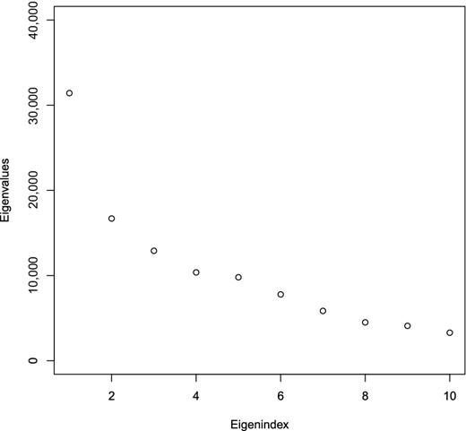
Leading eigenvalues of
In the left panel of Figure 5, we present the estimate of the top two eigenvectors of the covariance matrix , with colours indicating the genre of the song. The outliers in the -axis of this plot are particularly interesting: they reveal songs that polarise opinion among users (see Table 5) and that best capture variation in individuals' preferences for types of music measured by the first principal component. It is notable that Rock songs are overrepresented among the outliers (see Table 6), relative to, say, Country songs. Users who express a preference for particular songs are also more likely to enjoy songs that are nearby in the plot. Such information is therefore potentially commercially valuable, both as an efficient means of gauging users' preferences, and for providing recommendations.
![Plots of the first two principal components V^2prime (left) and the associated scores {u^i}i=1n (right) [Colour figure can be viewed at https://dbpia.nl.go.kr]](https://oup.silverchair-cdn.com/oup/backfile/Content_public/Journal/jrsssb/84/5/10.1111_rssb.12550/1/m_rssb_84_5_2000_fig-5.jpeg?Expires=1750218786&Signature=bstlqjXG3lYp8Ajo2HCkZadR861SphgQq4B3lI9OjB6UPJ00a6bE~2u71GPOXgfJTebBNiqAGwjDI2yDsEnMgOiisGcVCWADvpkh1YXVktuG~WaMcjb4ctPYWQWdn5fgDMXzEGUslTgky~RMEiMiL6rRv0MWdaTNEQL4QLpTFoaNvwZ5qXCvlCzjJqsUfiuww8hiIADFhbd83C1mM-moM13Ov0VB-J6CzScL8IJbwl8FCmU0BhoMwHiwuc4H5ngGdONh3o02QXkuIEhjk7jFUdh2IKuIoQXmKO6R~a3L~Z4Mu31ldyGbLcpgHGQnN4Gxl8Nh6g2t9KafdX-CgBSLvQ__&Key-Pair-Id=APKAIE5G5CRDK6RD3PGA)
Plots of the first two principal components (left) and the associated scores (right) [Colour figure can be viewed at https://dbpia.nl.go.kr]
Titles, artists and genres of the 22 outlier songs in Figure 5
| ID | Title | Artist | Genre |
|---|---|---|---|
| 1 | Your Hand In Mine | Explosions In The Sky | Rock |
| 2 | All These Things That I've Done | The Killers | Rock |
| 3 | Lady Marmalade | Christina Aguilera / Lil' Kim/ | Pop |
| Mya / Pink | |||
| 4 | Here It Goes Again | Ok Go | Rock |
| 5 | I Hate Pretending (Album Version) | Secret Machines | Rock |
| 6 | No Rain | Blind Melon | Rock |
| 7 | Comatose (Comes Alive Version) | Skillet | Rock |
| 8 | Life In Technicolor | Coldplay | Rock |
| 9 | New Soul | Yael Naïm | Pop |
| 10 | Blurry | Puddle Of Mudd | Rock |
| 11 | Give It Back | Polly Paulusma | Pop |
| 12 | Walking On The Moon | The Police | Rock |
| 13 | Face Down (Album Version) | The Red Jumpsuit Apparatus | Rock |
| 14 | Savior | Rise Against | Rock |
| 15 | Swing Swing | The All-American Rejects | Rock |
| 16 | Without Me | Eminem | Rap |
| 17 | Almaz | Randy Crawford | Pop |
| 18 | Hotel California | Eagles | Rock |
| 19 | Hey There Delilah | Plain White T's | Rock |
| 20 | Revelry | Kings Of Leon | Rock |
| 21 | Undo | Björk | Rock |
| 22 | You're The One | Dwight Yoakam | Country |
Genre distribution of the outliers (songs whose corresponding coordinate in the estimated leading principal component is of magnitude larger than 0.07)
| Rock | Pop | Electronic | Rap | Country | RnB | Latin | Others | |
|---|---|---|---|---|---|---|---|---|
| Population (Total ) | ||||||||
| Outliers (Total ) |
| Rock | Pop | Electronic | Rap | Country | RnB | Latin | Others | |
|---|---|---|---|---|---|---|---|---|
| Population (Total ) | ||||||||
| Outliers (Total ) |
The right panel of Figure 5 presents the principal scores of the users, with frequent users (whose total song plays are in the top 10% of all users) in red and occasional users in blue. This plot reveals, for instance, that the second principal component is well aligned with general interest in the website. Returning to the left plot, we can now interpret a positive -coordinate for a particular song (which is the case for the large majority of songs) as being associated with an overall interest in the music provided by the site.
As discussed above, it may be the case that some of the entries that we have treated as missing in fact represent a user's aversion to a particular song. We therefore studied the robustness of our conclusions by replacing some of the missing entries with an interest level of 1 (i.e. the lowest level available). More precisely, for some , and independently for each user , we generated , and assigned an interest level of 1 to uniformly random chosen songs that this user had not previously heard through the site. We then ran primePCA on this imputed dataset, obtaining estimators and of the two leading principal components. Denoting the original primePCA estimators for the two columns of by and , respectively, Table 7 reports the average of the inner product , where , based on 100 independent Monte Carlo experiments. Bearing in mind that the average absolute inner product between two independent random vectors chosen uniformly on is around 0.020, this table is reassuring that the conclusions are robust to the treatment of missing entries.
Robustness assessment: average inner products (over 100 repetitions) between top two eigenvectors obtained by running primePCA on the original data and with some of the missing entries imputed with an interest level of 1
| 0.05 | ||||
| 0.1 | ||||
| 0.2 |
| 0.05 | ||||
| 0.1 | ||||
| 0.2 |
Note: SEs are given in brackets.
6 DISCUSSION
Heterogeneous missingness is ubiquitous in contemporary, large-scale data sets, yet we currently understand very little about how existing procedures perform or should be adapted to cope with the challenges this presents. Here we attempt to extract the lessons learned from this study of high-dimensional PCA, in order to see how related ideas may be relevant in other statistical problems where one wishes to recover low-dimensional structure with data corrupted in a heterogeneous manner.
A key insight, as gleaned from Section 2.2, is that the way in which the heterogeneity interacts with the underlying structure of interest is crucial. In the worst case, the missingness may be constructed to conceal precisely the structure one seeks to uncover, thereby rendering the problem infeasible by any method. The only hope, then, in terms of providing theoretical guarantees, is to rule out such an adversarial interaction. This was achieved via our incoherence condition in Section 3, and we look forward to seeing how the relevant interactions between structure and heterogeneity can be controlled in other statistical problems such as those mentioned in the introduction. For instance, in sparse linear regression, one would anticipate that missingness of covariates with strong signal would be much more harmful than corresponding missingness for noise variables.
Our study also contributes to the broader understanding of the uses and limitations of spectral methods for estimating hidden low-dimensional structures in high-dimensional problems. We have seen that the OPW estimator is both methodologically simple and, in the homogeneous missingness setting, achieves near-minimax optimality when the noise level is of constant order. Similar results have been obtained for spectral clustering for network community detection in stochastic block models (Rohe et al., 2011) and in low-rank-plus-sparse matrix estimation problems (Fan et al., 2013). On the other hand, the OPW estimator fails to provide exact recovery of the principal components in the noiseless setting. In these other aforementioned problems, it has also been observed that refinement of an initial spectral estimator can enhance performance, particularly in high SNR regimes (Gao et al., 2016; Zhang et al., 2018), as we were able to show for our primePCA algorithm. This suggests that such a refinement has the potential to confer a sharper dependence of the statistical error rate on the SNR compared with a vanilla spectral algorithm, and understanding this phenomenon in greater detail provides another interesting avenue for future research.
1 When , we have that is the sine of the acute angle between and . More generally, is the sum of the squares of the sines of the principal angles between the subspaces spanned by and .
2 In R, we set the random seed to be 2019 before generating .
3 To be completely precise, in our simulations, and were generated independently (and independently of all other randomness) and were drawn from Haar measure on ; however, these matrices were then fixed for every replication, so it is convenient to regard them as deterministic for the purposes of this description.
4 In fact, to try to improve the numerical stability of the EM procedure, we prevented the sample covariance estimators from exiting the cone of positive semi-definite matrices during iterations and took Moore–Penrose pseudoinverses with eigenvalues below regarded as 0. Both of these modifications did indeed improve the algorithm, but some instability persists. Moreover, use of the SWEEP operator (Beaton, 1964), which is designed to compute the Schur complement in a numerically stable way, failed to remedy the situation, yielding identical (increasing) log-likelihood trajectories as the vanilla algorithm.
5 Each iteration of the EM algorithm involves the inversion of matrices, where the dimension of the th such matrix is (i.e. ). Using standard matrix inversion algorithms, then, each iteration has computational complexity of order , and moreover the number of iterations required for numerical convergence can be very large in higher dimensions. This meant that even when , primePCA was nearly 50 times faster than the EM algorithm.
ACKNOWLEDGEMENTS
The authors thank the anonymous reviewers for helpful feedback, which helped to improve the paper. Ziwei Zhu was supported by NSF grant DMS-2015366, Tengyao Wang was supported by EPSRC grant EP/T02772X/1 and Richard J. Samworth was supported by EPSRC grants EP/P031447/1 and EP/N031938/1, as well as ERC grant Advanced Grant 101019498.
REFERENCES
Author notes
Funding information Engineering and Physical Sciences Research Council, Grant/Award Numbers: EP/N031938/1; EP/P031447/1; EP/T02772X/1; H2020 European Research Council, Grant/Award Number: 101019498; NSF, Grant/Award Number: DMS-2015366
