


Abstract
This paper presents methods to estimate the number of persons with HIV in North Carolina jails by applying finite population inferential approaches to data collected using web scraping and record linkage techniques. Administrative data are linked with web-scraped rosters of incarcerated persons in a non-random subset of counties. Outcome regression and calibration weighting are adapted for state-level estimation. Methods are compared in simulations and are applied to data from the US state of North Carolina. Outcome regression yielded more precise inference and allowed for county-level estimates, an important study objective, while calibration weighting exhibited double robustness under misspecification of the outcome or weight model.
1 INTRODUCTION
Calculating estimates for rare or dynamic populations is challenging when no single data source contains all information necessary for estimation. A lack of a viable sampling frame further precludes the use of conventional methods for estimating the size and characteristics of a rare or ever-changing population. Record linkage techniques allow for multiple data sources to be combined, which can facilitate indirect estimation of the target population (Harron et al., 2017; Qayad & Zhang, 2009; St. Sauver et al., 2011). In the era of big data, these techniques can combine multiple types of data, including administrative records and publicly available data gathered through web scraping applications. However, when one or more data source is incomplete and record linkage results in missing data, methods are needed to generalize findings based on linked records to the target population (Bohensky et al., 2010; Ford et al., 2006; Harron et al., 2014; Judson et al., 2013).
The goal of this study is to develop and evaluate methods to estimate the number of incarcerated persons living with HIV in the US state of North Carolina (NC) jails overall and within each of the 100 counties over a fixed period of time by applying finite population inferential approaches to data collected using web scraping and record linkage techniques. Without information on this population, it is difficult to plan and implement programs to support the health of people living with HIV while in jail. Estimates of HIV within and across county jails in the state could be used by jail administrators as well as by local and state public health officials in efforts to ensure the availability of adequate medical resources to treat HIV during periods of jail incarceration and to support incarcerated persons’ health needs as they are released and return to the community.
NC does not maintain a list of persons living with HIV who are incarcerated in jails. To estimate the size of this rare population, jail incarceration records were linked with state court records and confidential NC health department records of persons in the state known to be living with HIV. This record linkage process provides estimates for the number of incarcerated persons living with HIV in jails in the 25 counties with consistently available jail incarceration data that includes sufficient information for accurate record linkage. The characteristics of the counties with publicly available data likely differ from those without publicly available data, so care must be taken when generalizing these results to the entire state of NC.
In this paper, two methods are considered for estimating the total number of incarcerated persons in NC jails living with HIV. One of these methods also provides county-level estimates within the 75 counties that either do not have publicly available jail rosters or whose rosters provide insufficient detail for record linkage. Both methods use sampling inference approaches that leverage county-level characteristics, either via outcome regression or weight calibration modelling. In Section 2, the methods are presented. Section 3 describes a simulation study comparing these methods based on bias and precision, and Section 4 provides an illustration of the two approaches using data from NC. Section 5 concludes with a discussion of the results and outlines the limitations of our study.
2 METHODS
2.1 Web scraping and record linkage
To generate estimates of the number of people living with HIV in NC jails who were charged with crimes within a NC county between 1 July 2018 and 30 June 2019, the following data sets were linked using incomplete personal identifiers: jail incarceration records derived from published inmate rosters available from 25 counties, statewide court records and confidential statewide health department records of persons living with HIV. A database of jail incarceration records was created using a technique called web scraping, in which, several times a day, automated ‘bots’ collected individual-level incarceration data from jail rosters published on county jail websites. In NC, 25 of the 100 counties had such online rosters consistently available, which include the incarcerated persons’ full names and ages (or dates of birth, DOBs). DOBs were consistently available in 16 counties and ages were included in the remaining 9 counties’ rosters. The 25 counties with available jail rosters are depicted in Figure 1. Over the 12-month period of study, this process generated approximately 177,000 incarceration-level records.

Availability of jail rosters by NC county.
State criminal court records were obtained from the NC Administrative Office of the Courts. These records include variables such as defendants’ full names, DOBs, the last four digits of their Social Security numbers (SSNs) and the county court system in which defendants’ cases were adjudicated. Over the 12-month period of study, there were over 1 million defendant-level records in the 25 counties with online inmate-level rosters and nearly two million defendant-level records for the entire state of NC. Finally, the NC State Health Department maintains a confidential database of all living persons who were diagnosed with HIV in the state. Among other variables, this database includes individuals’ full names, DOBs, SSNs and dates of HIV diagnoses. This database tracks lab results and access to care indicators for people living with HIV in NC.
Record linkage was conducted in two stages. During the first stage, our research team linked the jail and court records for the 25 counties with publicly available jail data. During the second stage, the NC Department of Public Health (DPH) linked the court records with their confidential HIV database for all 100 counties. Matching was conducted independently by the two research groups to ensure confidentiality of the DPH data. Linkage procedures differed in the two stages due to differing resources and priorities of the research groups. Following linkage, DPH provided deidentified, linked data to our research team. From the final linked data, the number of defendants and HIV-positive defendants in each of the 100 counties was computed. Additionally, the number of HIV-positive persons incarcerated and the proportion of defendants who were incarcerated were derived for the 25 counties with available incarceration data. Each of these steps is described in more detail below. Additional county-level covariates were obtained for analysis, as further discussed in Section 2.2.
A deterministic data linkage of jail and court records was performed using last names, partial first names, DOBs or ages, and counties. Deterministic matching was used for efficiency in the matching process and to reduce the potential of false matches. Deterministic matching did not require a manual review of potential matches, which would be logistically prohibitive given the number of records linked. The courts and jails are highly integrated within counties, as they are often physically connected and routinely share data. For this reason, all jail-court matches were constrained to be in the same county, reducing the probability of false matches. Thus, only incarceration records that corresponded with a court case in the same county were included in this analysis. For example, incarceration records associated with individuals temporarily held in jails who were charged at the federal rather than state level (e.g. due to immigration violations) would not match to county-level court records and therefore are not considered part of the target population. In the jail and court matching, 11% of incarceration records did not match to a court record in the corresponding county and were thus not included in subsequent analyses. The distribution of non-linked records across the 25 counties is shown in Web Table 1. With the exception of one county that accounted for approximately 14% of total incarcerations but 22% of non-linked incarcerations, the distribution of non-linked incarcerations in each county tracked fairly closely with the distribution of incarcerations overall. Because individuals could have multiple charges brought against them and/or could have been incarcerated multiple times during the study period, the jail to court linkage was a many-to-many matching.
DPH then linked the court records for all 100 counties to the State’s database of HIV records using the software package Link Plus 3.0 to apply their internal probabilistic matching algorithm. Matching was based on first and last name, year of birth and the last four digits of the SSN. DPH accepted matches with Link Plus probability scores of 25 or greater as true matches. DPH subsequently performed a thorough manual review of the matching, including comparisons with deterministic linkage results, and found little substantive differences between the deterministic and probabilistic matching procedures in this application. The DPH matching process was commensurate with the process employed to match their own records used for public health interventions.
Following linkage with HIV records, DPH provided linked and deidentified incarceration and court records. In the final matched data set, 63 HIV-infected persons were linked to multiple defendants. This represented less than 1% of HIV-positive court defendants on the file. There was one instance in which two records from the HIV database were linked to the same incarceration record. This incarceration record and the two linked HIV cases were removed from our analysis. All linkage results from the three data sources were subsequently aggregated at the person level. Using these aggregated linked data, we derived the previously discussed quantities needed for the estimation procedures described below. The Internal Review Board at the University of North Carolina at Chapel Hill reviewed and approved the study protocol (IRB # 17-0946).
2.2 Estimation
Denote the total number of incarcerated persons with HIV in NC jails who were charged with crimes within a NC county over the fixed period of interest by and within each of the N = 100 NC counties by , i = 1, …, N such that . The inferential goal is to estimate and for i = 1, …, N. Within each county i, denote the number of HIV-positive defendants by and the proportion of HIV-positive defendants who were incarcerated by , such that . Note was derived as described in Section 2.1 for all N counties, and was derived through the jail-court record linkage process for the n = 25 counties with publicly available jail rosters containing ages or DOBs. Thus, was derived from record linkage for the n counties that have publicly available jail rosters. For the purposes of this paper, the estimates resulting from record linkage are treated as known quantities. That is, error in the record linkage process is assumed to be negligible and is ignored. Furthermore, the 100 counties are assumed to be independent. Without loss of generality, assume that counties are ordered such that is known for i = 1, …, n and unknown for i = n + 1, …, N.
The 25 counties with available jail rosters are heavily concentrated in the central and western regions of the state (Figure 1), and so it is likely that the characteristics of these counties differ from those without publicly available data. Two statistical methods for obtaining estimates of are considered, each of which aims to reduce bias in generalizing the non-random sample of n counties to the entire state by leveraging county-level characteristics. The outcome regression approach aims to estimate in the N − n counties where this quantity is unknown, and thus also provides estimates for within these counties. The weight calibration approach uses a weighting adjustment to estimate directly and does not provide county-level estimates.
Both approaches leverage county-level covariates thought to be associated with the proportion of HIV-positive defendants who were incarcerated (for outcome regression) or the number of HIV-positive persons incarcerated in each county and the availability of jail rosters (for weight calibration). County-level covariates included the following, obtained from Vera Institute’s publicly available ‘Incarceration Trends’ dataset for the year 2014: annual jail admissions, daily jail populations, index crime rates and poverty levels (Vera Institute of Justice, 2014). County urbanicity level was based on NC Rural Center classifications, which define counties as rural if the 2010 US Census estimated population density per square mile was 250 people or fewer (NC Rural Center, 2021). The number of unique defendants and HIV-positive defendants obtained from record linkage are used as county-level covariates, as are the political affiliations of the district attorneys associated with each county and the number of traffic tickets issued per 100 county residents. The later two covariates were obtained from state and national public data sources (North Carolina Conference of District Attorneys, 2021; North Carolina Judicial Branch, 2021; North Carolina State Board of Elections, 2021; United States Census Bureau, 2021). The selection of covariates for each approach is discussed in Section 4.
2.2.1 Outcome regression
The outcome regression approach follows the prediction-based paradigm for finite population inference (Lohr, 2010, p. 148) by using in the n counties with publicly available jail rosters to estimate the proportions in the remaining N − n = 75 counties without publicly available rosters, based on a set of predictors. To estimate , the following linear regression model is fit for the n counties with publicly available rosters: , where represents the 1 × m vector of covariates for county i, β is the m × 1 vector of model parameters, and with errors independent across counties. The model outcome was not transformed because values of were not expected to be close to the boundaries of the parameter space, and this model demonstrated reasonable fit for data from NC (see Section 4.1).
Predicted values and 95% prediction intervals (PIs) ( , ) are obtained from the fitted model for each of the N − n counties without publicly available jail rosters. Let be the 97.5th percentile of the t-distribution with n − m degrees of freedom. Then and and are the lower and upper limits of
where are the maximum likelihood estimates for β, X is the n × m matrix of predictors for the regression model from the n counties with publicly available jail rosters, and the mean squared error is used to estimate .
To estimate the number of persons with HIV incarcerated in jails in each of the N − n counties without publicly available jail rosters along with 95% PIs, the predicted proportions and PI limits are multiplied by the number of HIV-positive defendants in the county. That is, point estimates and the lower and upper endpoints for the 95% PIs are defined as follows, respectively: , , and .
An estimate for the total number of incarcerated persons with HIV in NC jails can be obtained by adding the known number of incarcerated persons with HIV in the n counties to the estimated number of incarcerated persons with HIV in the N − n counties without publicly available jail rosters:
The estimator ((1)) is unbiased and has minimum variance among the class of all unbiased estimators of under the assumed linear regression model above (Bolfarine & Zacks, 1992, pp. 31–32). Let be the (N − n) × m matrix of covariates for the N − n counties without publicly available jail rosters, , and I be the (N − n) × (N − n) identity matrix. Then, a 95% confidence interval (CI) for is: , where (Bolfarine & Zacks, 1992, p. 122). Note is unbiased even if ε is not normally distributed, provided the error terms are independent, mean zero and homoscedastic; the additional assumption of normality justifies the validity of the confidence interval above (Bolfarine & Zacks, 1992, p. 122).
2.2.2 Weight calibration
Weight calibration aims to balance an observed sample with respect to a set of calibration variables by constructing the weights such that sample sums of the weighted calibration variables equal the population totals of the calibration variables (Deville & Särndal, 1992; Folsom & Singh, 2000). Weight calibration can reduce selection bias resulting from missing data under the assumption that each missed observation had some unknown (but positive) probability of participating in the study (Kott & Liao, 2015), and can reduce the variance of an estimated total compared to estimation based on uncalibrated weights when the outcome of interest is correlated with calibration variables (Deville & Särndal, 1992). When applied to correct for non-response or missing data, weight calibration is a type of selection modelling as well as a quasi-randomization based technique, as pseudo selection probabilities are estimated using external data (Kott, 2006; Valliant, 2020).
Weight calibration can be used to estimate . Calibrated weights are computed for each of the n ‘responding’ counties (i.e. the counties for which publicly available jail rosters were available) via a generalized exponential model (Folsom & Singh, 2000; Kott, 2006), where an a priori set of covariates assumed to be associated with response and the outcome of interest are calibrated to known state-level totals. When weight calibration is applied to probability sampling designs, each unit is assigned an initial weight that accounts for its probability of selection. Here, because no random sampling of counties occurred, each of the N counties is assigned an initial weight of 1 (i.e. , i = 1, …, N). That is, each county initially represents itself when combining county-level estimates to form an overall estimate for NC. To account for non-responding counties, the weight for each responding county i is adjusted by , the reciprocal of its probability of response. Assume where
is the m × 1 vector of calibration model parameters; and are specified by the analyst and determine the lower and upper bounds of the adjustments, respectively; is a centring constant for the model; and (Folsom & Singh, 2000; Kott, 2006; RTI International, 2012). For this application, a logistic model is assumed for the response probabilities by setting, (essentially unbounded), and . This implies , that is each county’s probability of response is approximately equal to a logistic function of the calibration variables (Kott, 2006).
Let be the response status for county i, with if county i responded, otherwise. Let be the m × 1 vector of calibration variable totals for the finite population (i.e. all 100 counties in NC). That is, . The parameter is then estimated by finding that solves the set of calibration equations using Newton-Raphson. After solving the calibration equations, is the calibration adjusted weight for responding county i (i = 1, …, n). Thus, the weighted sample totals of the calibration variables equal the population totals. When an intercept is included in the calibration model, corresponding to letting for i = 1, …, N, = .
The total number of incarcerated persons with HIV in NC jails is estimated by the following calibration estimator:
The estimator (2) is doubly robust, in that it is asymptotically unbiased for the finite population total if or if the linear model holds, where has mean zero (Kott, 2006; Kott & Liao, 2012). A linearization variance estimator is
where (Kott, 2006). A finite population correction (FPC) adjustment (1 − n/N) can be made to (3) to account for the large percentage of observed counties (n/N = 25/100) (see, e.g. Kish, 1965, p. 43). The FPC-adjusted variance estimator is . A 95% CI for is (RTI International, 2012), where replaces to obtain an FPC-adjusted CI.
3 SIMULATION STUDY
A simulation study was conducted to examine the two estimation approaches under both correct and incorrect model specification. True values of and were generated for each of the N = 100 counties (as outlined below), as well as three sets of response probabilities that allow for the examination of three sample size scenarios. In addition, larger finite populations of N ∈ {200, 500} were simulated, each with the same response probability distributions specified for the N = 100 population. While the n = 25, N = 100 scenario is of most relevance to the application presented in Section 4, the additional simulation scenarios provide insight regarding the performance of these methods if applied to other settings where the sample and/or finite populations were larger.
For the N = 100 population, the covariates and the number of defendants () from the linked data file were used. For the N ∈ {200, 500} populations, the data file was duplicated, with each county appearing either twice (for N = 200) or five times (for N = 500). Normally distributed random noise was added to continuous covariates and to the number of defendants in each county to obtain larger finite populations with counties that were similar, but not identical, to the observed data for the 100 NC counties.
3.1 Correct model specification
Given the covariates for each county, a true was generated for each of the counties in the finite population (N ∈ {100, 200, 500}) as , where was an urbanicity indicator variable, was the square root transformed index crime rate and was the square root transformed percent below poverty value for county i. The error term was generated from a mean zero normal distribution, that is , where σ = 0.015. The resulting had a median of 0.15 and ranged from 0.11 to 0.23 for N = 100, from 0.07 to 0.24 for N = 200 and from 0.03 to 0.29 for N = 500. The range of simulated was comparable to the range of the observed in the NC data. These values were used to calculate a true number of incarcerated persons with HIV within each county, resulting in ranging from 0 to 224 for N = 100, from 0 to 232 for N = 200 and from 0 to 243 for N = 500, with a sum of (for N = 100), (for N = 200) and (for N = 500).
For each finite population size (N ∈ {100, 200, 500}), three sets of response probabilities were generated for each county according to the model . Three values of were chosen such that the mean response across the counties for the three simulation scenarios was 0.25 (), 0.50 () and 0.75 (). This resulted in expected sample sizes for N = 100 of n = 25 (the number of responding counties in NC), 50 and 75. For N = 200, this resulted in expected sample sizes of n = 50, 100 and 150. For N = 500, this resulted in expected sample sizes of n = 125, 250 and 375.
After generating true values under the specified models, 2000 simulated samples were selected for each of the nine finite population and sample size scenarios. Simulated samples were obtained by assigning each county a binary response status based on a random draw from a Bernoulli random variable with mean . After the response status was assigned, and thus were observed only for the responding counties, and the outcome regression and weight calibration methods were implemented with correctly specified models to estimate and/or . Because the same covariates were included in the data generating mechanism for and , both the outcome and weight models were correctly specified when , and were included in the models. For each iteration of the simulation, (1) and (2) were calculated along with estimated standard errors. Additionally, 95% CI and 95% PI coverage were evaluated.
The simulation results are summarized in Table 1 for each of the nine finite population size by sample size combinations under correctly specified models. Density plots for the distribution of (1) and (2) across the 2000 simulated samples for N = 100 are shown in Figure 2; results for the N ∈ {200, 500} populations were similar and are not shown. Empirical bias was small (absolute mean percent bias of 2.1% or lower) for all sample sizes, finite population sizes and methods. The largest empirical bias was for the weight calibration method when N = 100 and n = 25, the scenario of most interest for the application. Among the remaining scenarios, absolute mean percent bias ranged from 0.0% to 0.7% of the true value. For all population and sample sizes, the distributions of both estimators were centred close to the true value of (depicted with vertical dotted lines in Figure 2).
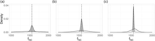
Density plots for estimates of based on outcome regression (dark grey) versus weight calibration (light grey) with correctly specified models, 2000 simulations, N = 100, (a) n = 25, (b) n = 50 and (c) n = 75.
Simulation summary results with correctly specified models, 2000 simulations
| N | Avg n | Method | Avg | Empirical bias (%) | ASE | ESE | SER | 95% CI Coverage (%) | 95% CI HW |
|---|---|---|---|---|---|---|---|---|---|
| 100 | 25 | OR | 1556 | 0.0 | 51 | 49 | 1.0 | 98 | 106 |
| WC | 1524 | −2.1 | 241 | 358 | 0.7 | 79 | 498 | ||
| WC-FPC | 1524 | −2.1 | 208 | 358 | 0.6 | 76 | 431 | ||
| 50 | OR | 1556 | 0.0 | 26 | 22 | 1.2 | 98 | 52 | |
| WC | 1552 | −0.2 | 205 | 163 | 1.3 | 95 | 412 | ||
| WC-FPC | 1552 | −0.2 | 144 | 163 | 0.9 | 90 | 290 | ||
| 75 | OR | 1556 | 0.0 | 14 | 12 | 1.1 | 99 | 27 | |
| WC | 1562 | 0.4 | 184 | 86 | 2.1 | 99 | 366 | ||
| WC-FPC | 1562 | 0.4 | 91 | 86 | 1.1 | 95 | 182 | ||
| 200 | 50 | OR | 3082 | 0.7 | 62 | 58 | 1.1 | 96 | 124 |
| WC | 3046 | −0.5 | 503 | 494 | 1.0 | 92 | 1012 | ||
| WC-FPC | 3046 | −0.5 | 436 | 494 | 0.9 | 88 | 876 | ||
| 100 | OR | 3074 | 0.4 | 35 | 33 | 1.1 | 96 | 69 | |
| WC | 3062 | 0.0 | 377 | 270 | 1.4 | 98 | 748 | ||
| WC-FPC | 3062 | 0.0 | 266 | 270 | 1.0 | 93 | 529 | ||
| 150 | OR | 3068 | 0.2 | 20 | 19 | 1.0 | 96 | 39 | |
| WC | 3063 | 0.0 | 322 | 154 | 2.1 | 100 | 636 | ||
| WC-FPC | 3063 | 0.0 | 160 | 154 | 1.0 | 95 | 317 | ||
| 500 | 125 | OR | 8573 | −0.1 | 89 | 88 | 1.0 | 95 | 177 |
| WC | 8568 | −0.1 | 898 | 790 | 1.1 | 96 | 1778 | ||
| WC-FPC | 8568 | −0.1 | 777 | 790 | 1.0 | 93 | 1538 | ||
| 250 | OR | 8576 | 0.0 | 52 | 53 | 1.0 | 95 | 103 | |
| WC | 8588 | 0.1 | 656 | 442 | 1.5 | 100 | 1292 | ||
| WC-FPC | 8588 | 0.1 | 463 | 442 | 1.0 | 96 | 913 | ||
| 375 | OR | 8578 | 0.0 | 31 | 31 | 1.0 | 95 | 61 | |
| WC | 8593 | 0.2 | 554 | 250 | 2.2 | 100 | 1089 | ||
| WC-FPC | 8593 | 0.2 | 277 | 250 | 1.1 | 97 | 545 |
For outcome regression, the average estimated standard error approximately equalled the empirical standard error. The outcome regression CIs were conservative for the smallest finite population N = 100, but the empirical coverage was close to the nominal 95% for the larger finite populations. The weight calibration method exhibited undercoverage when N = 100, n = 25, regardless of whether or not the FPC adjustment was made. For larger finite population sizes and sampling fractions, weight calibration tended to be conservative when the FPC was ignored and provided close to nominal coverage when the FPC was applied.
The outcome regression estimator was more precise (Figure 2, Table 1), with average estimated standard errors 4.7–17.9 times smaller than the weight calibration estimator without the FPC adjustment and 4.1–8.9 times smaller than the weight calibration estimator with the FPC adjustment. Likewise, the outcome regression 95% CI half-widths were much smaller than the weight calibration half-widths for all population and sample size scenarios. County-level PIs for the outcome regression approach had close to nominal coverage, as 94%–95% of PIs included the true across the 2000 simulated samples for each scenario (results not shown).
3.2 Incorrect model specification
Additional simulations were conducted to evaluate the performance of these methods under misspecified outcome and/or weight calibration models. For these simulations, the data were generated according to the models and , where , , and are as defined in Section 3.1 and for mean responses {0.25, 0.50, 0.75}, respectively, for N = 100, with slight adjustments for N ∈ {200, 500} to ensure the appropriate mean response. The simulation study described in Section 3.1 was repeated under this data generating mechanism, but with the following modifications. For the ‘weight model incorrect’ simulations, and were included in the assumed outcome regression and weight calibration models, and for the ‘outcome model incorrect’ simulations, and were included in the assumed models. For the ‘both models incorrect’ simulations, was included in the assumed models, where represents the estimated prevalence of HIV in county i, derived by dividing the count of residents who were HIV-positive (North Carolina HIV/STD/Hepatitis Surveillance Unit, 2017) by the estimated number of county residents in 2016 from the US Census Bureau (U.S. Census Bureau Population Division, 2018). This variable was moderately correlated with , and , but was not part of the data generating mechanism for or .
The incorrect model specification simulation results are presented in Figure 3 and Web Tables 2–4. Mean empirical bias for each finite population and sample size scenario under each form of model misspecification is shown in Figure 3. As expected, the outcome regression method had minimal empirical bias when the outcome model was correctly specified (Figure 3), but exhibited considerable bias when the outcome model was misspecified (Figure 3 and Figure 3). The weight calibration estimator exhibited minimal empirical bias when either model was misspecified (Figure 3 and Figure 3), but was biased when both models were misspecified (Figure 3). This is expected due to its doubly robust property. The largest relative empirical bias for the weight calibration estimator when one model was misspecified occurred when N = 100, n = 25 and the weight model was misspecified (−4.7%).
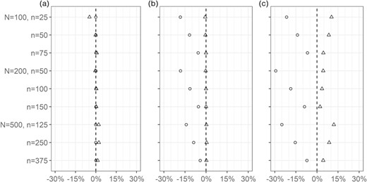
Mean empirical bias (%) for estimates of based on outcome regression (circle) versus weight calibration (triangle) with incorrectly specified models, (a) weight model incorrect, (b) outcome model incorrect, (c) both models incorrect.
Empirical coverage of 95% CIs tended to be less than the nominal level when the assumed models were misspecified. When the outcome model was misspecified, 95% CI coverage for the outcome regression method ranged from 0% to 56% across the scenarios considered (Web Tables 3 and 4). When the FPC adjustment was not applied and either model was correctly specified, coverage for the weight calibration method was close to or exceeded the nominal 95% level for all but two scenarios (N = 100, n = 25 and N = 200, n = 50) (Web Tables 2 and 3). However, when the FPC adjustment was applied, coverage was typically below the nominal level. Coverage for the weight calibration method was closer to the nominal level than the outcome regression method when both models were misspecified for all scenarios, regardless of whether the FPC was applied (Web Table 4). As with the simulations in Section 3.1, outcome regression estimates were more precise and resulting CIs were narrower than CIs corresponding with the weight calibration method across the three model specifications considered (Web Tables 2–4).
The simulations described in Sections 3.1 and 3.2 provide insight regarding the performance of the statistical methods specified in Section 2 under correctly and incorrectly specified models for varying finite population and sample sizes. The outcome regression approach had good empirical properties when the outcome model was correctly specified, with the estimator empirically unbiased and the corresponding CIs and PIs having empirical coverage rates approximately equal to the nominal level. The weight calibration estimator was much less precise than the outcome regression estimator but was more robust to model misspecification.
4 RESULTS
The outcome regression and weight calibration methods were implemented on the linked NC data, as outlined in Section 2. Annual jail admissions, daily jail populations, index crime rates, the number of defendants per county and the number of traffic tickets per 100 county residents were square root transformed to reduce skewness of these variables and thus the overinfluence of the largest or outlier counties on model fit.
4.1 Outcome regression
The covariates a priori thought to be predictive of were poverty level, daily jail population, number of unique defendants in court records, the political affiliation of the district attorney and the number of traffic tickets issued per 100 county residents. These covariates were included in the multivariable outcome regression model. Because was small in many counties, was estimated based on all defendants, not just defendants living with HIV. This is justified under the assumption that the risk of incarceration for defendants is independent of their HIV status. The second sensitivity analysis discussed below considers violations of this assumption. The known and estimated in the 25 counties for which the outcome regression model was fit aligned fairly well (Figure 4), indicative of reasonable model prediction. Additionally, diagnostic plots based on residuals showed no evidence of violations to the model assumptions (Figure 4 and Figure 4). Table 2 presents the parameter estimates from the model. Daily jail population and number of unique defendants in court records were both associated with the outcome; however, these covariates were strongly correlated (estimated Spearman correlation coefficient = 0.93), so the estimates in Table 2 should be interpreted with caution.
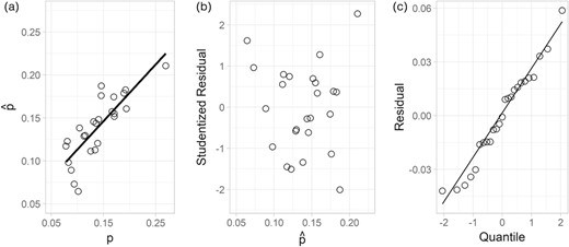
Diagnostic plots for multivariable regression analysis in Section 4.1 (a) predicted versus actual proportion of defendants who were incarcerated, (b) studentized residuals versus predicted values, (c) normal Q–Q residual plot.
Parameter estimates for multivariable outcome regression model
| Variable | 95% CI | p | ||
|---|---|---|---|---|
| Intercept | 0.173 | 0.057 | (0.055, 0.292) | 0.01 |
| Percent below poverty | 0.001 | 0.002 | (−0.004, 0.006) | 0.73 |
| Daily jail populationa,b | 0.305 | 0.068 | (0.164, 0.446) | <0.001 |
| Unique defendants in court recordsa,b | −0.037 | 0.007 | (−0.052, −0.022) | <0.001 |
| District attorney political affiliation: Republican | 0.018 | 0.015 | (−0.014, 0.050) | 0.26 |
| Traffic tickers per 100 populationb | −0.009 | 0.016 | (−0.043, 0.025) | 0.57 |
In thousands.
Square-root transformed.
Based on the multivariable model, were computed and the number of HIV-positive persons incarcerated within the 75 counties without publicly available jail rosters, , were estimated. As an example, county-level estimates and 95% PIs for the 5 largest and 5 smallest non-responding counties in NC are displayed in Table 3. Based on the outcome regression approach, for the time period of 1 July 2018 through 30 June 2019, , with a 95% CI of (1339, 1533).
Estimated number of persons with HIV in jails in the five smallest and five largest non-responding counties from 1 July 2018 through 30 June 2019
| County | , 95% PI | , 95% PI | |
|---|---|---|---|
| Small county 1 | 1 | 0.16 (0.07, 0.25) | 0.2 (0.1, 0.3) |
| Small county 2 | 1 | 0.17 (0.10, 0.25) | 0.2 (0.1, 0.2) |
| Small county 3 | 5 | 0.07 (0.00, 0.22) | 0.3 (0.0, 1.1) |
| Small county 4 | 3 | 0.15 (0.06, 0.24) | 0.4 (0.2, 0.7) |
| Small county 5 | 19 | 0.10 (0.00, 0.21) | 2.0 (0.0, 4.1) |
| Large county 1 | 64 | 0.14 (0.07, 0.21) | 9.1 (4.8, 13.4) |
| Large county 2 | 105 | 0.10 (0.04, 0.17) | 10.8 (3.9, 17.7) |
| Large county 3 | 171 | 0.08 (0.01, 0.15) | 13.2 (1.6, 24.8) |
| Large county 4 | 241 | 0.14 (0.06, 0.21) | 33.0 (15.5, 50.6) |
| Large county 5 | 403 | 0.10 (0.01, 0.18) | 38.5 (5.5, 71.5) |
Two sensitivity analyses were conducted. In the first analysis, subsets of predictor variables were considered and observations were removed to assess robustness of the findings to the inclusion of different covariate sets and influential or outlier counties, respectively. One county was highly influential in the model based on Cook’s distance while another county had much larger than the other observed counties, so the model was fit again twice, individually excluding these counties. The resulting estimates and 95% CIs were similar for all models examined, with within ±5.4% of the estimate based on the multivariable model from Table 2. Web Table 6 presents the models considered in this sensitivity analysis and the resulting estimates. In the second sensitivity analysis, violations of the assumption that the risk of incarceration for defendants is independent of their HIV status were considered. Within each of the 25 observed counties, the value of used in the outcome regression model was specified as , where represents the proportion of all defendants who were incarcerated and c represents a constant, with c > 0. Note the primary analysis is the special case where c = 1. The estimate and its corresponding CI was computed for c ranging from 0.5 to 2.0, with the results presented in Web Figure 1. For this range of c, was between −15.9% and 31.8% of the estimate based on the multivariable model from Table 2.
4.2 Weight calibration
County-level covariates a priori thought to be associated with the availability of jail rosters and the number of incarcerated persons with HIV were the number of unique defendants in court records, the number of HIV-positive defendants in court records, annual jail admissions, daily jail population, index crime rate and urbanicity status. Responding counties tended to have more total defendants and HIV-positive defendants compared to non-responding counties (Table 4). Annual jail admissions, daily jail populations and index crime rates were also higher in responding counties than non-responding counties. Non-responding counties were more rural compared to responding counties.
County characteristics by response status, N = 100 counties
| County characteristic | Responding counties n = 25 | Non-responding counties N − n = 75 | |
|---|---|---|---|
| Unique defendants in Court recordsa | Median (Q1, Q3) | 24.6 (14.5, 49.6) | 9.1 (4.6, 17.0) |
| Mean (SD) | 38.1 (34.6) | 13.3 (12.3) | |
| Min, Max | 3.3, 115.3 | 1.0, 64.9 | |
| HIV+ defendants in Court records | Median (Q1, Q3) | 88 (45, 202) | 20 (9, 64) |
| Mean (SD) | 209 (275) | 48 (66) | |
| Min, Max | 3, 955 | 0, 403 | |
| Annual jail admissionsa | Median (Q1, Q3) | 6.5 (3.5, 12.6) | 1.6 (0.5, 3.1) |
| Mean (SD) | 9.7 (10.3) | 2.5 (2.7) | |
| Min, Max | 1.5, 40.3 | 0.0, 12.9 | |
| Daily jail population | Median (Q1, Q3) | 230 (139, 488) | 87 (36, 176) |
| Mean (SD) | 404 (435) | 123 (111) | |
| Min, Max | 46, 1881 | 0, 521 | |
| Index crime ratea | Median (Q1, Q3) | 3.8 (1.7, 7.1) | 1.3 (0.3, 2.7) |
| Mean (SD) | 7.2 (9.3) | 1.7 (2.1) | |
| Min, Max | 0.6, 40.0 | 0.0, 14.5 | |
| Urbanicity status | Rural | 12 (48%) | 68 (91%) |
| Regional city, suburban | |||
| County or urban | 13 (52%) | 7 (9%) |
In thousands.
The weight calibration estimator (2) was calculated using covariates listed in Table 4. The annual jail admission covariate was excluded from the calibration model due to collinearities with the other covariates that resulted in a lack of model convergence. Based on the simulation study, the sample size of n = 25 counties is not large enough to ensure nominal coverage of 95% CIs, and undercoverage was made worse when the FPC adjustment was applied. For this reason, the FPC was excluded from the standard error calculation. The multivariable calibration model parameter estimates are included in Table 5. The calibrated weights exhibited a fairly high amount of variation, ranging from 1.0 to 19.8 (with a median of 2.1). Note with the constraints of the lower bound equal to 1 and that the weights sum to 100, the possible bounds for the calibrated weights were 1 to 76. Two counties had calibrated weights over 10, with the remaining 23 counties having calibrated weights less than 10. The calibration weights for each of the 25 responding counties are included in Web Table 5, along with the covariates from the weight calibration model associated with each county. Based on the calibrated weights, , with a 95% CI of (1400,1687) for the 1 July 2018 to 30 June 2019 time period.
Parameter estimates for weight calibration model
| Variable | 95% CI | p | ||
|---|---|---|---|---|
| Intercept | 5.61 | 1.97 | (1.55, 9.67) | 0.01 |
| Urbanicity: regional city, suburban county or urbana | −0.58 | 1.16 | (−2.98, 1.82) | 0.62 |
| Unique defendants in court recordsb | 0.29 | 0.94 | (−1.65, 2.23) | 0.76 |
| HIV+ defendants in court records | 0.01 | 0.01 | (0.00, 0.03) | 0.13 |
| Daily jail populationb | −3.17 | 6.42 | (−16.42, 10.08) | 0.63 |
| Index crime rateb | −3.69 | 3.68 | (−11.28, 3.91) | 0.33 |
Rural is the reference level.
In thousands, square-root transformed.
The estimates of are similar for the outcome regression and weight calibration methods, with overlapping CIs. The precision of the two methods differs greatly, with outcome regression providing the narrower interval (half-width of 97) and weight calibration providing a wider interval (half-width of 143).
5 DISCUSSION
While web scraping is a commonly used method for collecting data, use of web scraping remains a relatively novel public health approach to measure health outcomes, and the linking of web-scraped data with confidential public health records is rare. To our knowledge, this study represents the first study to leverage such a linkage to estimate HIV prevalence in any setting. Record linkage across three large NC databases, combined with outcome regression or weight calibration, allows for indirect estimation of a rare population that cannot be directly measured given the current data collection practices and capabilities of NC jails. Measurement of this population can support public health interventions to ensure care for HIV while persons are incarcerated.
There are advantages and limitations of each method that are specific to the application at hand. Outcome regression has the advantage of producing county-level estimates, which will be useful for targeting HIV interventions where they are most needed. However, outcome regression approaches rely on correct outcome model specification (Hansen, 1987), and simulations demonstrated large empirical bias when the outcome model was incorrectly specified. Weight calibration can also be used to obtain an overall estimate for the entire state of NC. The weight calibration estimator is doubly robust, providing asymptotically unbiased estimates if either the outcome model or the response model is correctly specified. Furthermore, unlike the outcome regression approach, weight calibration does not require the error terms to be homoscedastic or normally distributed. However, the weight calibration method does not provide county-level estimates and simulation results suggest the corresponding confidence intervals of the population total may under cover in settings similar to the NC jail example. In the simulations, the FPC was applied to the calibration model variance estimator without a formal justification. Use of the FPC led to improved CI coverage compared to ignoring the FPC adjustment for larger finite populations under correct model specification.
There are limitations associated with our findings. The small sample of 25 counties made model-fitting challenging and the validity of asymptotic approximations questionable. The two evaluated approaches treat the number of HIV-positive defendants and persons with HIV in the 25 jails as known quantities, ignoring any error in the record linkage process. The results of this analysis may be sensitive to linkage error. The use of deterministic matching of the jail and court records could result in missing some true matches due to typos or incomplete identifiers in the data sources. For some of the variables included in the outcome regression and/or weight calibration models, there was a lack of overlap between responding and non-responding counties. For example, there were two non-responding counties with daily jail populations of zero, but the minimum daily jail population for responding counties was 46. This lack of overlap may introduce bias in the estimates of the number of persons with HIV in NC jails; however, the inclusion of multiple covariates in both the weight calibration and outcome regression models potentially mitigates such bias. Furthermore, while limiting the jail to court matching within counties reduces the potential for false matches, it excludes incarcerated individuals who did not have charges against them in the same county.
Despite these limitations, these findings demonstrate how outcome regression and weight calibration can be used to account for missing data following record linkage procedures in order to generalize results to a target population. These methods can be used for continued estimation of the number of incarcerated persons living with HIV in NC jails over time. Additionally, the methods could be applied to data from other US states and in different settings to estimate the burden of public health conditions (e.g. opioid use) within the jail and prison systems. More broadly, the findings reflect the potential to generate public health insights through the novel aggregation of data and its linkage to confidential health information. As in the current example, similar efforts in the future will be dependent on close collaboration and strong trusting relationships between academia and public health practitioners.
SUPPLEMENTARY MATERIALS
The supplementary materials include tables summarizing the non-linked incarceration records across NC counties and detailed results from the simulation study with incorrectly specified models as described in Section 3.2. Additionally, a supplemental table with covariates from the weight calibration model and resulting weights for each of the 25 counties with publicly available jail rosters is included. A table and figure display the results of the sensitivity analyses described in Section 4.1. SAS and SUDAAN code for computing the two estimators along with the corresponding standard error estimators is available at https://github.com/bonnieshook/Record_Linkage_Finite_Pop_Inference.
Supporting Information
Additional supporting information may be found in the online version of the article at the publisher’s website.
ACKNOWLEDGEMENTS
This work was supported by the US National Institutes of Health under award numbers R01 AI129731, R01 AI157758 and R37 AI029168, and by the University of North Carolina at Chapel Hill Center For AIDS Research (CFAR), an NIH-funded programme P30 AI050410. The content is solely the responsibility of the authors and does not necessarily represent the official views of the National Institutes of Health. The authors thank the Joint Editor, Associate Editor, two anonymous reviewers, Phillip Kott at RTI International for their helpful suggestions which improved the paper and Mincen Liu at the University of North Carolina at Chapel Hill for help with data preparation. We also gratefully acknowledge Erika Samoff and Brad Wheeler from the Communicable Disease Branch of the NC DHHS for their important contributions to this project.
