


Summary
The consequences of reduced fertility and mortality on the age distribution are an issue for most developed countries, but especially for the ‘Asian tiger’ economies. We use functional data analysis forecasting techniques to project the population of Hong Kong. Our projections include error estimates that allow for forecasting error as well as exogenous variations of fertility and migration numbers. We separate out the effects of pure demographic shifts from projected behavioural changes in labour force participation. This enables us to look at the kinds of changes in labour force participation that would be required to offset the aging effects that we estimate.
1. Introduction
Population aging is a global challenge. It is the inevitable consequence of very high post-war fertility followed by much lower fertility in an environment of steadily reducing mortality. World wide, the proportion of adults aged 65 years and older increased from 5.1% in 1950 to 5.9% in 1980, but it has since reached 8.3% in 2015 and is expected to increase to 15.8% by 2050. Such trends are clearest in high income countries. The starkest example is Japan where it is already 26%, and which has one of the lowest fertilities and longest life expectancies in the world (United Nations, 2017).
There are several measures of the economic burden of population aging in common use. The elderly dependence ratio is the number of elderly divided by the number of productive people, where the productive people are equated with the age range 15–64 years. Since this ignores the burden of the young, we shall prefer to look at the number of non-productive (i.e. young and old) per productive people, which we call the age dependence ratio (ADR). This has been called the total dependence ratio by some researchers. We shall point out some of the consequences of using this measure in Section 9.1.6. Any measure based on equating a crude age range with productivity takes no account of changing patterns of work in response to aging. Indeed, in most countries where aging is a problem, labour force participation rates (LFPRs) are increasing among the elderly whereas educational credentialism is leading to lower participation in the 15–19 years range. Therefore, we prefer to replace the crude age group surrogate with actual labour force participation, and to integrate across all ages to obtain the overall labour force participation. Of course, this requires data on, and projections of, age- and gender-specific labour force participation rates, which is why it is less commonly used. We call this the economic dependence ratio (EDR), though we note that Yip et al. (2010) used this term for the odds against participation.
Aging patterns are especially pronounced in the highly developed Asian countries, namely Japan, South Korea, Singapore, Taiwan and Hong Kong. Although Japan is 15 years ahead of the others, all are projected to have of the order of 35% aged over 65 years old by 2050. The pace and magnitude of aging are expected to be faster and deeper than the European experience, largely because of their common experience of extreme fertility decline. The total fertility rate (TFR) in these five Asian countries dropped from around five children per woman to below replacement (2.1) in only 25 years and collapsed to below 1.4 thereafter. Although pronatalist policies are in place, these Asian countries show no sign of the fertility rebound that has been seen in Europe. Meanwhile, decreasing trends are observed in their LFPRs among males, partly offset by increasing rates for females (International Labour Organization, 2015).
As the trend is well established, interest is moving from the extent and timing of the demographic transition to how countries can better prepare (Bouvier, 2001; Nagase and Brinton, 2017). What kinds of changes to labour force patterns are required to offset aging and to what extent can fertility recovery and immigration reverse the trend itself?
Hong Kong is our chosen case-study of the potential effect of aging in the high income Asian context. With a dense population of 7.4 million, a TFR at 1.2 and life expectancy among the highest in the world, Hong Kong underwent a rather extreme version of demographic transition over recent decades (Yip et al., 2001, 2009; Census and Statistics Department, 2016). There are also two special and interesting features of Hong Kong demography.
Firstly, since the large-scale refugee migrations from mainland China in the 1930s, Hong Kong has always been a ‘migrant metropolis’ and mainland immigrants continue to be a major source of overall population growth. Currently, there is a daily intake of 150 migrants from mainland China known as ‘one-way permit holders’ (OWPHs), mostly the spouse or child of a Hong Kong resident. Although the main purpose is family reunion, OWPHs are eligible for permanent residency after 7 years. Because of the very low fertility in Hong Kong, the one-way permit (OWP) scheme has been the major source of population growth and has contributed to over 60% of population growth in the past decade. Most OWPHs are in the productive age range (80.5% were aged 15–64 years in 2014) and are mainly female (66.6%), which mitigates the aging effects of low fertility and mortality.
Secondly, cross-border marriage is a very unique situation in Hong Kong. Since the 1997 change of sovereignty, Hong Kong has become a special administrative region of the People's Republic of China (PRC) and is governed under the so-called one country–two systems. There is a physical border between Hong Kong and the PRC. PRC residents do not have the automatic right of abode in Hong Kong. The term ‘cross-border marriage’ means a marriage between a Hong Kong resident and a PRC resident. It has become a substantial component of Hong Kong marriage, especially with the increasing business and social contact since 1997. At its peak, 45% of marriages registered in Hong Kong involved a mainland spouse, but this has been levelling off and is now about 35%. The majority of cases involve Hong Kong men marrying mainland women, which has imposed a shortage of local male marriage partners for local females: a point that has not been recognized or addressed in other studies.
In this paper, we provide 50-year projections of Hong Kong's total population, including particularly the age structure and various EDRs. There are several noteworthy technical features of this work.
- (a)
We use functional data analysis (FDA) (Ramsay and Silverman, 2005) to project mortality, fertility, labour force participation and net migration. This technique is currently underutilized in demography and has several advantages. For instance, projected fertility and mortality curves are automatically smooth and the uncertainty of population projections is easily simulated.
- (b)
We address the gender imbalance constraints on the Hong Kong population due to female overrepresentation in immigration from the PRC. We quantify the effects of this imbalance, which is caused by, but can also be mitigated by, cross-border marriages and include projections of these cross-border marriages in our model.
- (c)
In assessing the effects of aging on EDRs, we separate out the effects of pure demographic shifts from projected behavioural changes in labour participation. This allows us to look at the kinds of change in labour force that would be required to offset projected aging effects. We supplement our projections with scenario analyses where fertility and net migration are exogenously varied and find that one of these has much more effect than the other.
The plan of the paper is as follows. We give a short overview of functional data analysis. We then use this technique to model and predict fertility, mortality, labour force participation and migration flow, all treated as (smooth) functions of age for each gender. We then use these projections to project the Hong Kong population. We also generate projections under a range of plausible scenarios where fertility and migration flows are manipulated exogenously and evaluate the age burden as measured by the ADR and EDR. The policy implications are discussed in the final section.
2. Projecting functional data
Our projections involve fertility, mortality, labour force participation rates and migration, all of which depend on age. FDA treats these demographic features as functions, generically denoted by f(x), where x here represents age. We expect that f(x) is a smooth function of x and that the ‘shape’ of f(x) will change smoothly over time. FDA has been available for several decades but its application to demography was first highlighted by Hyndman and Ullah (2007). A systematic review on the application of FDA identified 84 references post 1995 (Ullah and Finch, 2013): only three in the field of demography. One was an application to Serbia (Nikitovic, 2011) and one an unpublished report on Great Britain (Shang et al., 2013).
2.1. Functional data model
We have observations ft(xj) at time points t = 1,…,T and ages x1,…,xq. We arrange this as a T × q matrix with rows indexing time and columns age. For instance, for our mortality data we have q = 86 ages ranging from x1 = 0 to x86 85 years and greater and T = 39 time points from 1976 to 2014. Our goal is to make m-step-ahead projections fT+m(xj).
A simple but naive method is to analyse each age xj separately, i.e. to take each column of the data matrix, to fit a time series model to ft(xj) and to project this into the future. This leads to forecasts that quickly become a non-smooth function of xj. The idea of FDA is to describe the systematic changes in ft(xj) in terms of a small number (often two or three) of smooth features and to project these into the future. This not only reduces statistical uncertainty because we use two or three forecast models instead of q models but also generates forecasts which mirror the smoothness of the historical data. It also provides a parsimonious way to describe how the curve has changed, and will change, over time.
With FDA, the basic observations are the rows ft(x) and these functions are described with a single equation
for some value K<min(q,T). So the function ft(xj) at time t is generated by a baseline mean function μ(xj) plus a time progressing linear combination of K basis functions ϕk(xj). The case K = 1 is the well-known model of Lee and Carter (1992). For applications where ft(x) is thought to be a smooth function of x, it is recommended to presmooth each row of the data matrix first.
2.2. Fitting
For a given K, the basis functions ϕk and the coefficients βt,k are estimated by singular value decomposition (SVD). Further theoretical details are in the on-line appendix A.
As in other modelling contexts, the fit improves with more components K, either measured by the total squared error or the sum of the first K eigenvalues of the SVD. If the main aim of the decomposition is forecasting then components can also be rejected on the basis of their contribution to the forecast; for those components whose coefficients βt,k are white noise (or a random walk) the forecasts of these coefficients will be 0 (or quickly decay to 0). It is common for this to occur and for only a small number of components to be retained.
2.3. Forecasting
Forecasts are generated by applying univariate time series methods to each of the k sequences βt,k. By construction, these series are orthogonal and are modelled separately. Forecasting these K series is the part of analysis where art as well as science are required, though automatic time series algorithms are available, such as auto.arima in R which we shall utilize where appropriate.
It is common to measure the accuracy of a forecasting procedure conditionally on model selection. In this case, model selection is deemed to include extraction of the basis functions, so only the estimates of the future βt,k involve statistical error, measures of which are routinely outputted by the time series package that is used. Moreover, estimated from equation (1) the squared standard error of the m-step-ahead forecast is
A useful feature of FDA methods is that this standard error can be used to generate estimates of the statistical uncertainty of our final projections. To incorporate the uncertainty in our forecasts we simulate the population by using where z is drawn from the standard normal distribution.
3. Fertility rates
3.1. Historical patterns in fertility rates
We obtained data for 34 years (from 1981 to 2014) on the age-specific fertility rate (ASFR), age of mother being measured to the nearest year. Fertility is measured in units of live births per 1000 females and is taken to be 0 outside the age range 15–49 years.
Foreign domestic helpers are an important population component in Hong Kong, numbering more than 320000 in 2017. They are overwhelmingly female and come mainly from the Philippines, Indonesia and other relatively low income countries in south and south-east Asia. The wage is relatively affordable (US $550 per month) compared with the median household income (US $3300 in 2017). On average there is one foreign domestic helper per eight households and they provide much needed elderly and child care support to Hong Kong families (Census and Statistics Department, 2017). However, they have no right of abode in Hong Kong; nor do their children. For this reason, they are best considered as a separate population and fertility rates are computed after excluding them from the database.
Fig. 1(a) plots the ASFR functions ft(x) against age x for each year, darker lines being the most recent. The curves have been moving towards the right, representing delay of childbearing. Total fertility, which is the area under the curve, is in Fig. 1(b) and decreased steadily from 1981 to 2001. The rebound from 2002 appears impossible to anticipate from the previous data and some might argue that it is impossible to predict rates accurately in the future, since they are partly driven by social trends that are inherently complex. This is supported by the erratic behaviour of the TFR over the last 3 years.
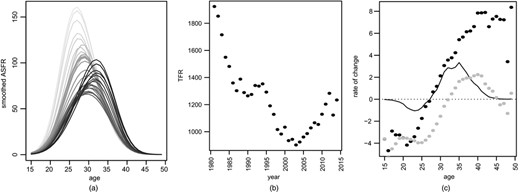
Historical fertility: (a) historical ASFRs 1981–2014 (smoothed); (b) TFR versus time showing rebound from 2002; (c) percentage growth over the previous 34 years ( ) and the most recent 15 years (
 ) (
) ( , absolute growth rate over the previous 15 years
Fig. 1(c) shows the rate of change of fertility by age. The grey points give the percentage change over the previous 34 years. Rates decreased for all ages up to 32 years but mostly increased at ages above 32 years. The dark points give the percentage change over the previous 15 years. It appears that fertility rates have increased even more strongly at all ages above 28 years whereas the tendency of decreasing rates at lower ages is still apparent. These are all percentage rates of change and suppress the absolute change. The full curve shows the absolute growth in ASFR over the previous 15 years. Most of the increase in TFR is attributable to higher absolute rates in the age range 30–40 years (which have grown at about 3% per annum), partly offset by decreases for ages 20–25 years.
3.2. Functional data decomposition of fertility rates
The panel of fertility rates was log-transformed then smoothed (as recommended by Hyndman and Ullah (2007)) by using a 7 degrees-of-freedom smoothing spline. The back-transformed data were displayed earlier in Fig. 1(a). FDA was applied to the smoothed log-data and two clear components emerged, accounting for 95% of the variation. Moreover, all subsequent components have coefficients βt,k that follow white noise or a random-walk process and so contribute nothing to long-run forecasts. Plots of these components and the time varying coefficients βt1 and βt2 are in Fig. 13 of the on-line appendix B.
The first component describes a tendency for higher fertility rates for mothers over 32 years old with a peak around 40 years of age and reduced rates at young age groups. The coefficients βt1 have been increasing strongly over time, though at a reducing rate. The second can be interpreted as a combination of two effects, namely higher TFRs with a simultaneous shift to the right. So increasing βt2 will increase the TFR but also skew the ASFRs towards older mothers. These coefficients decreased consistently from 1981 to 2002 and then strongly rebounded, which is a very similar pattern to what we saw in the raw historical TFR.
3.3. Functional data forecasts of fertility rates
The FDA decomposition models the historical ASFR curves by using two easily interpreted components and reduces forecasting these curves to forecasting the two sequences of coefficients βt1 and βt2.
For the first sequence βt1, the forecast is based on a power model with auto-regressive AR(1) errors and is displayed in the upper right-hand panel of Fig. 13 in the on-line appendix B. The second component is much more difficult to forecast. We have already noted the erratic behaviour of the TFR in the last 3 years of the historical data and the same variability is present in βt2. Details of our ensemble forecast model are in the on-line appendix B.
Fig. 2(a) shows historical data in grey and 50 years of FDA projections in shades of blue. The centre of the ASFR curve is projected to move to the right by another 3 years over the next 50 years. Fig. 2(b) shows the projection 50 years hence. Fig. 2(c) shows the projections of TFR with error bands generated by simulation. The first component, which measures increases in fertility for mothers over 32 years of age, is well estimated. It is the total fertility which is less certain. These wide bands indicate that the TFR is difficult to estimate and in later sections we shall interpret this to mean that fertility is best investigated by varying it exogenously in our simulations rather than measuring uncertainty by statistical error.
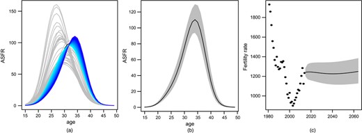
Projected fertility: (a) projected ASFRs (pale grey curves are from 1981 to 2014; forecasts are from 2015 to 2064 starting light blue and ending dark blue); (b) forecast ASFR function in 2064 with 1-standard-error bands; (c) TFR from summing the projected ASFRs at the left-hand side, with standard error bands
The value of FDA here may appear nebulous. However, the shapes of the ASFR curves are well estimated and this is important in our projections since population dynamics will depend on how these curves integrate with the age distribution of mothers. The large standard error of the TFR warns us of the limitations of forecasting total fertility while still allowing quite precise forecasts of ASFR.
4. Mortality rates
We obtained data on registered deaths from 1976 to 2014, broken down by age and gender, and converted these into mortality rates by dividing by the age- and gender-specific mid-year population. The single-age population data that we used have an open age group 85 years and older. Fig. 3(a) shows mortality rates averaged over the 39-year period for males (the full curve) and females (the broken curve), both log-transformed. Fig. 3(b) shows the absolute reduction between 1976 and 2014. Further detailed data displays are in the on-line appendix C.
4.1. Historical patterns in mortality rates
Males have higher mortality than females at almost all ages but mortality is reducing for both genders and at all ages, largely because of improvement in hygiene and advances in medical technology. Hong Kong has a universal and affordable healthcare system. The decreases are largest for older age groups and for males, where there is more potential for improvement. These patterns will be detected and projected in our FDA decomposition.

Historical mortality rates per 1000 population: (a) average age- and gender-specific mortality rates (1976–2014), LN(rates) versus age ( , males;
  , females); (b) reduction in mortality rates from 1976 to 2014 (, males;
  , females)
Mortality rates were log-transformed and then presmoothed from age 1 to 84 years, using a smoothing spline with 15 degrees of freedom. Age group 85 years and older was not included since it represents a discontinuity and age 0 was also treated separately since it is drastically higher than for age 1 year.
4.2. Functional data forecast of mortality rates
FDA was applied to the smoothed log-transformed data. The first component explains 90.5% and 90.1% of the variation for males and females respectively. The variation that is explained by the second component drops to 3.5% and 4.1%. For both males and females, subsequent components are governed by coefficients βt,k that are either white noise or some other stationary process for which forecasts will quickly decay to 0.
The first two components are displayed in Figs 15 and 16 in the on-line appendix C for males and females respectively. The decompositions are quite similar. The first basis function is uniformly negative and describes a tendency for mortality rates generally to reduce, and at a faster rate for younger than older people. The coefficients βt1 have steadily increased over the past four decades (the top right-hand panel of Fig. 15) but at a decreasing rate. The second component describes a tendency for lower mortality for ages around 20 years with a simultaneous increase for children around the age of 10 years. For both genders, the coefficients βt2 were decreasing until the mid-1990s. This means that, on top of the general decreasing tendency described by component 1, mortality for children around 10 years was reducing faster than the long-term trend and for those around 20 years was reducing slower than the long-term trend. These effects reversed in the mid-1990s, reflecting a faster mortality reduction for those around 20 years and slower for those around 10 years old.
We used a two-component model for the forecast of mortality rates. The time series for βt1 and βt2 were carefully modelled (see the on-line appendix C). βt1 is projected to continue to increase but at a decreasing rate. The second component will eventually decay but still has some effects in the following decade, suggesting additional reductions in mortality in ages around 20 years and less for children around 10 years old . The smoothed historical mortality rates as well as a 50-year projection on the log-scale are displayed in Fig. 4.
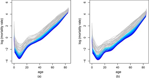
Projected mortality rates for males and females (pale grey curves are 1976–2014 data; forecasts from 2015 to 2064 start light blue and end dark blue): (a) historical and projected mortality rates per 1000 for males on a log-scale; (b) historical and projected mortality rates per 1000 for females on a log-scale
5. Labour force participation
We obtained data on the LFPR by age group and gender from 1994 to 2014. For reasons that were explained in Section 3, foreign domestic helpers are considered as a separate population and excluded from the analysis. A summary of the main patterns in the data is displayed in Fig. 5. Fig. 5(a) displays rates for males and females by age group, averaged over time. Fig. 5(b) shows recent growth rates for each age group and both genders. Further data displays are in the on-line appendix D.
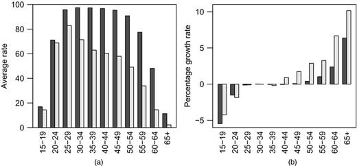
Historical LFPRs (, males;  , females) (source, Census and Statistics Department, Hong Kong Special Administrative Region): (a) average rates 1994–2014 for males and females by age group; (b) percentage growth rates from 2004 to 2014 in LFPR odds for various age groups
The broad patterns are easy to summarize. For males, rates are near saturation in the 25–49 years age range whereas rates for females almost match those for males from 15 to 24 years but then fall short, reaching a peak of 84% in the 25–29 years age group and decreasing thereafter. Single-figure estimates of trends for the last 10 years only are in Fig. 5(b). For both genders, rates have decreased strongly for the 15–24 years group: more so for males. The decrease is probably due to improving education opportunities and higher levels of training that are required in the modern economy. For both genders rates have increased at higher ages. However, for females this growth is much stronger (albeit off a lower base) and applies to middle as well as older ages.
To avoid extrapolating outside the range (0, 1), we first applied the logit transform to all rates. We applied a 7 degrees-of-freedom smoothing spline and interpolated to individual ages from 15 to 70 years. This gives a 21×56 data matrix for each gender.
5.1. Functional data forecast of rates for males
Two components account for 97.5% of the variation and for subsequent components the βt,k follow a random-walk or white noise process. The two chosen components are displayed in Fig. 18 of the on-line appendix D. In plain language, the first component describes a tendency of increasing participation for the elderly and decreasing participation for those under 45 years old. This tendency has steadily increased over time. The second component describes a more general tendency for the LFPR curve to shift to the right. The tendency is smaller in magnitude and has mainly been increasing over the past 10 years.
The time varying coefficients βt1 and βt2 were carefully modelled (see the on-line appendix D) and the projections with error bands are also indicated in the right-hand panels of Fig. 18.
As expected from the projections and interpretations of the βt,k, the male LFPR as a function of age is projected to decrease for ages below 50 years but increase for ages above 50 years. Although the total LFPR depends on the age distribution, it appears as if this will decrease. The smoothed historical data as well as 50 years of projection are displayed in Fig. 6 for easy comparison with the rates for females, to which we now turn.
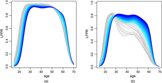
Projected LFPRs for males and females (pale grey curves are 1994–2014 historical data; forecasts from 2015 to 2064 start light blue and end dark blue): (a) historical and projected LFPRs for males on a logit scale; (b) historical and projected LFPRs for females on a logit scale
5.2. Functional data forecast of rates for females
We know that the rates for females are strongly increasing in the central age groups and we have seen that the rates for males are decreasing and are projected to continue to decrease. This raises the prospect that forecasting the rates for females will exceed those for males and this indeed occurs for quite-well-supported forecast models of the females data. We considered it unlikely that the total rates for females will surpass those for males, though this has already happened for the youngest ages where rates for both genders are quite low.
Fig. 19 in the on-line appendix D shows the historical differences between the rates for males and females on the logit scale (in grey). These have also been projected by using FDA with a method that limits how far logit rates for females may exceed those for males. Details are in the on-line appendix. Combining the forecasts of the difference with the forecasts for males produces forecasts for females. These are displayed on the logit scale in the on-line appendix and on the ordinary scale in Fig. 6.
6. Migration
Hong Kong has two qualitatively different migration channels, namely two-way flows of Hong Kong permanent residents (HKPRs) and one-way inflow of migrants from mainland China, known as OWPHs. Their different natures result in distinct age and gender patterns. This justifies separate analyses.
HKPRs have freedom to move into and out of Hong Kong. The OWP is issued by the PRC Government granting PRC residents the right to leave the mainland permanently and to move to Hong Kong or Macau. They are eligible for permanent residence after 7 years. There has been a long-standing daily quota of 150 people (54750 per annum). Although the primary purpose of the scheme is family reunion instead of general immigration, OWPHs have become a significant constituent of population growth in Hong Kong. The scheme has undergone recent amendments. Since April 2011, ‘overage children’ (aged over 18 but less than 60 years) of HKPRs who live in the PRC may apply for an OWP. Previously, this was limited to children under 18 years old.
6.1. Net movement of Hong Kong permanent residents
We obtained data on net movement (inflow minus outflow) of HKPRs by gender and single age (up to 85 years or older) from 2007 to 2014. On average, the net movement was −49332 per annum, with slightly more males moving out than females (female-to-male ratio 0.92). However, this is misleading: until 2013, around 64% of this net movement were babies, overwhelmingly born in Hong Kong to mainland women with non-resident fathers, known locally as type II babies. According to law, these babies were entitled to permanent residence at birth. Between 91% and 99% return to mainland China before 1 year of age, since their parents do not have residence right (Census and Statistics Department, 2011).
Since 2003, the number of type II babies increased enormously, peaking at 35700 in 2011 and accounted for nearly 40% of all births in that year. It is estimated that over 300000 type II babies were born. This was driven by mainland mothers visiting Hong Kong to give birth, partly to avoid the one-child policy and more generally to take advantage of the superior healthcare services for delivery and the right of abode of becoming a Hong Kong resident. This explains the huge outflow of HKPRs aged 0 in the data. Moreover, about 50% of these babies would return to Hong Kong before 6 years of age for schooling (Census and Statistics Department, 2011) though this has recently reduced to about 25% (Yip et al., 2017). Nonetheless, these flows ceased as a result of the zero-quota policy on obstetric services for mainlanders that was imposed by the Hong Kong Government in 2013, in response to severe strains on the local obstetric healthcare system. So, the earlier pattern for age 0 cannot be naively projected and some adjustments to the age 0 data are required. Further details are in the on-line appendix E. After adjustment, there were a net of 27059 HKPRs moving out of Hong Kong averaged over 8 years, with a female-to-male ratio of 1.08.
The data were then presmoothed, with age 0 excluded for reasons just explained. The smoothed data were then modelled by using FDA, which revealed two components accounting for 88.2% and 91.1% of total variation for males and females respectively. However, all four sequences of coefficients bt,k were best modelled as white noise, contributing nothing to the forecast. Fig. 7(a) displays the mean functions extracted from the FDA.
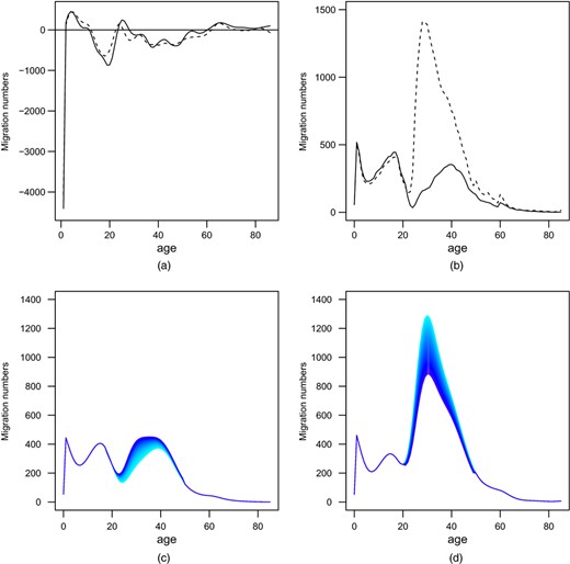
Migration numbers: (a) mean function of net movement of HKPRs ( , males;
  , females); (b) historical average numbers of inflow of OWPHs versus age for 2007–2014 (
 , males;
  , females); projected number of inflow of OWPHs versus age from 2015 to 2064, starting from light and ending in dark blue (c) for males and (d) for females
Future patterns of movement depend on numerous external factors that are difficult to predict. Historical trends should play an important role but no consistent trend has been identified. Therefore, we shall assume that future movement of HKPRs will stably follow the mean age–gender pattern, with a net number of 13057 females and 11992 males leaving Hong Kong each year. In our later projections, we vary total migration numbers exogenously.
6.2. Inflow of one-way permit holders
We obtained data on inflow of OWPHs by gender and single age (up to 85 years or older) from 2007 to 2014. Fig. 7(b) displays the age–gender pattern averaged over 8 years. Each year, there were an average of 44820 PRC residents holding OWPs who moved to Hong Kong, with a large 2.1 female-to-male ratio. Detailed displays of the data are in the on-line appendix E. Clearly, females aged 20–50 years are hugely overrepresented, driven by the large gender asymmetry in cross-border marriages. Historically, the rate of Hong Kong men marrying PRC women has been 5–6 times more frequent than the reverse, though the ratio is more like 2.5 in recent years.
The data were presmoothed and FDA extracted two components accounting for 96.6% and 96.2% of the total variation for males and females respectively. The gender-specific mean functions revealed that the large inflow of females occurred within childbearing ages 21–49 years. However, all time varying coefficients βt,k are white noise and therefore, as with the HKPR decomposition, have zero contribution to the forecast. On the basis of this, we could project the simple averages in Fig. 7(b) into the future. However, we prefer a less naive approach.
Future inflow of OWPHs will be influenced by two drivers, neither of which is predictable statistically. The first is the number of families requiring reunion. This is driven by cross-border marriage which is in turn driven by the gap between quality of life in Hong Kong compared with in mainland China. Historically, this meant mainland women marrying Hong Kong men. The number of such marriages is already diminishing as the differential in living standard reduces. It is reasonable to assume that this trend will continue and drive a decrease in the inflow of female OWPHs of childbearing age. In contrast, the number of inflow of adults may increase because of the overage children policy that was mentioned at the start of this section. Consequently, we may observe the female-to-male ratio moving towards parity in the future.
Making use of the difference of male and female mean functions (μF(xj)−μM(xj)) identified from the FDA, we proposed a mathematical model to project the future inflow of OWPHs, considering a change in gender ratio and a change in age distribution at the same time. Details of the model are in the on-line appendix E and projections are displayed in Figs 7(c) and 7(d), with daily number ranging from 115 to 124 and the gender ratio decreasing from 1.93 to 1.36. We do not have a measure of forecast error for these projections. However, migration numbers will be varied exogenously in Section 8 .
7. Population projections
On the basis of our forecasts of fertility, mortality and migration flows we project the Hong Kong population by using the standard cohort component method. All projections are supplemented by estimates of statistical error.
7.1. Projection method
For each year we first apply mortality rates to each gender–age segment by using random binomial generation, i.e. if n people are subject to mortality p then we generate a binomial count with these parameters. This assumes that deaths occur independently, both within and between the groups. The amount of random variation that is involved is typically small because of the large counts involved, but it does accumulate over the 50 years of our projection.
We next apply fertility rates to females to generate births by using the same binomial method. However, we do not include every female in the 15–49 years age range: why? In 2014, the ratio of females to males was 1.07. This is forecast to increase strongly, reaching 1.15 by 2030 and 1.25 by 2050. The gender skew is not driven by differences in mortality, which mainly affect older age groups, but by a strong skew towards females in net immigration. It is not clear whether or not all females in Hong Kong will find a partner when the gender ratio is 1.25. In contrast, it might be argued that there is an effectively inexhaustible supply of males from the PRC. This is an issue that has not been identified in the literature and is not easy to resolve, but it does have a non-trivial effect on projections depending on how it is handled. In the on-line appendix F we detail our approach to this issue, which involves looking at trends in cross-border marriages for males and females and making reasonable projections. We also give some results on the level of difference that this whole issue can make to overall projections.
For the final steps of our projections, we apply net immigration flow excluding OWPHs to each age–gender group and lastly OWPHs to each age–gender group.
Statistical variability is accounted for by using the FDA standard errors. For each simulated projection, we perturb the forecast fertility, mortality and LFPR profiles with their standard errors multiplied by a standard normal variable. We summarize 1000 runs of this procedure using the mean and 1-standard-deviation bands either side.
7.2. Demographic projection
Fig. 8 describes our results. Fig. 8(a) shows the total population for 2015–2064, as well as disaggregated numbers in three age groups. Notionally, we deem the youngest age group to be economically inactive. In the previous literature, the economically active group has often been taken to be aged 15–65 years; however, with increasing participation, as forecast in Section 5, it seems preferable to extend this to 15–70 years.
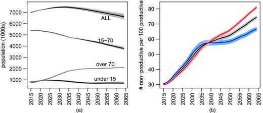
Projected population counts and ADR: (a) summary of 1000 projections using best forecasts of all drivers ( , mean;
  , 1 standard deviation); (b) summary of projections of ADR (
 , males;
  , females;
  , both genders)
The total population is projected to peak at 7.47 million in 2033. The numbers in the youngest age group will be relative stable. The main changes will be a decrease in the productive age range from 5.38 million to 3.79 million at the same time as the oldest age group increases from 0.75 million to 2.11 million. As described in Section 1, we measure age burden by the ratio of non-productive age groups (i.e. the youngest plus the oldest) to the productive age group, labelled ADR. Larger values indicate a larger burden. This has been displayed separately for males and females, and also overall, in Fig. 8(b). Not surprisingly, the females ratio is projected to become higher than the males ratio in around 2036, almost entirely driven by the lower mortality of females compared with males.
7.3. Economic participation projections
We combine the population projections with our forecast age- and gender-specific LFPR to investigate the effects of aging on overall labour force participation, known as EDR.
Let Lg(x,t) be the LFPR at time t, conditional on age =x and gender g≡m, f. We generated forecasts of Lg(x,t) in Section 3 Roughly speaking, for central ages, rates for females will tend to increase, and for males will tend to decrease slightly; the population will both age and tend to skew to females. It is not clear from this qualitative discussion how overall participation will fare.
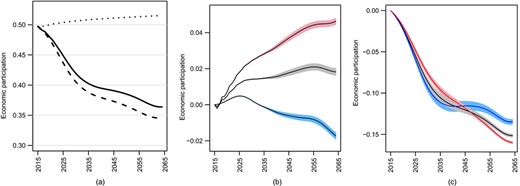
The EDR is obtained by integrating Lg(x,t) with respect to the age distribution πg(x,t) at time t. We denote this Eg(t); see the on-line appendix F for its exact definition. We have projected Eg(t) 1000 times, allowing for uncertainty in the forecasts of πg(x,t), and Lg(x,t) and summarized results by the mean. The full curve in Fig. 9(a) is for all genders and shows that E(t) will decrease from 50% to 37% by 2064. How much of this decline is due to demographic changes and how much to changes in age- and gender-specific LFPR?
Economic participation: (a) projections of E(t) ( , baseline projection;
  , projection with demographic changes only;
  , projection with changes in LFPR only); (b) effect on E(t) of changes in LFPR assuming fixed demographics (
 , females;
  , males); (c) effect of demographic changes on E(t) assuming fixed Lg(x) (
 , females;
  , males)
We can investigate this by holding either πg(x,t) or Lg(x,t) fixed at t = 0. Again, mathematical and notational details are in the on-line appendix F. The broken curve in Fig. 9(a) shows the mean value of our projections where only the demography πg(x,t) changes. This is projected to fall to under 35%, which is slightly worse than E(t) because we are not factoring in increases in LFPR, especially among the elderly. The dotted curve shows the mean value of our projections where only Lg(x,t) changes and demography is held fixed. This is projected to increase from 50% to 52%. So the short story is that underlying economic participation will increase modestly but will be easily outweighed by the effects of aging.
It is helpful to decompose the separate effects of demographics and LFPR by looking at the relevant differences. Formulae are again given in the on-line appendix F. The pure effect of changes in Lg(x,t) are displayed in Fig. 9(b). It shows the changes in economic participation if the age distribution was held constant at πg(x,0). Female participation (pink) would increase by about 0.045 and male participation (blue) would decrease by about 0.015. Overall, there would be an increase of 0.015 (grey). Fig. 9(c) shows pure effects of demography. The change is –0.12 for males and –0.16 for females. This is because aging of the female population is more pronounced than for the male population. These effects are almost an order of magnitude larger than the pure economic effects. The conclusion from this analysis is that demographics effects will swamp the forecast increased participation in older age groups and among females that has sometimes been touted as a solution to demographic aging.
8. Population scenarios
Our FDA decomposition of fertility and migration flows had time varying coefficients that followed random walks or white noise. This suggests that they are not statistically predictable; fertility is based on an accumulation of autonomous decisions which depend on economic and political trends; sometimes, net migration and especially OWPH flows are based on economic and political decisions. This being so, it seems pertinent to vary these two drivers exogenously by plausible amounts to see what effect they will have on ADRs and EDRs.
In this section we consider the effects of exogenous manipulations of fertility and migration on the age burden. This is measured by the ADR, which is the ratio of non-productive to productive people and the EDR, which is simply the overall labour force participation rate. We remind the reader that neither of these measures makes a distinction between young and old non-productive people.
8.1. Scenarios considered
Our baseline scenario and projection method is as described in the previous sections. Baseline fertility forecasts were described in Section 3.3 Current Chinese Government policy is to grant 50000 OWPS per year (though not all of these are always exercised) and we described forecasts of the demographics of these in Section 6.
We shall make three kinds of perturbation from the baseline forecast. The first is to multiply the whole set of fertility curves by 1+g/100. This amounts to an instantaneous and permanent change to fertility of g% and is termed fast. The second method is to multiply the fertility curves for the projection m years ahead by (1+g/100)m/50. This amounts to gradually changing fertility by g% over a period of 50 years and is termed slow. We chose g = ±25 which means that total fertility would be around 1.5 in the high case and a little below 1 in the low case, which seems historically reasonable. The third manipulation is to vary total OWPH numbers. We consider the effects of increasing this to 75000 or reducing it to 25000. Note that OWPHs tend to be in the productive 15–70 years age group and are skewed towards females, whereas increased fertility introduces non-productive children to the population and slightly favours males. The combinations of these manipulations are summarized in Table 1.
Projection scenarios considered†
| Scenario | Fertility change | OWPH change |
|---|---|---|
| 1 | None | None |
| 2 | 25% (s) | None |
| 3 | 25% (f) | None |
| 4 | −25% (s) | None |
| 5 | −25% (f) | None |
| 6 | None | 25000 |
| 7 | None | −25000 |
| 8 | 25% (f) | −25000 |
| 9 | −25% (f) | 25000 |
| 10 | 25% (f) | 25000 |
| 11 | −25% (f) | −25000 |
s means that fertility change is introduced slowly i.e. gradually over 50 years; f means that it is introduced fast, i.e. instantly in 2015.
8.2. Age dependence
Fig. 10 describes our results on the ADR. The first message from all of these plots is that the ADR is set to increase drastically over the next 50 years, regardless of fertility or migration levels.
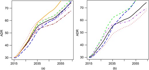
Effects of fertility and net flow on the ADR (the measure is the number of non-productive per 100 productive): (a) baseline scenario 1 ( ) with manipulations 2–7 (
 , scenario 2;
  , scenario 3;
  , scenario 4;
  , scenario 5;
  , scenario 6;
  , scenario 7); (b) baseline scenario 1 (
 ) with manipulations 8–11 (
 , scenario 8;
  , scenario 9;
  , scenario 10;
  , scenario 11)
Increased fertility is, perhaps surprisingly, associated with a higher, i.e. worse, dependence ratio. This is because our measure includes the young as dependent. Looking at the fast increase (scenario 3), the ADR increases and then begins to return towards baseline as the children enter the productive age range. After 50 years, it has just returned to baseline. The slow increase (scenario 2) is similar to the fast increase but delayed by about 25 years. Eventually, the age distribution will converge to a limit, but this limit is not reached in 50 years. Nor is it clear that the limiting ADR would be more favourable, even though the age distribution will certainly be younger, again because the young are counted as dependent.
Increasing or decreasing OWHPs lead to lower or higher dependence ratios, both immediately and persistently. This is as expected since the majority of OWPHs are in the economically active age range. It is interesting to note that, by around 2035, the dependence ratio for the increased OWHP scenario 6 falls below the fast fertility reduction scenario 5 and results in the lowest ratios into the future.
Fig. 10(b) describes the effects of the fast fertility and OWHP manipulations in combination. Scenarios 9 and 10, which both have an increase in OWHP, lead to the lowest dependence ratios. The two differ in the fast fertility manipulation which has an initial effect but appears to be largely swamped by the OWHP manipulation by the end of the forecast period. Scenarios 8 and 11, which both have a reduction in OWHP, lead to the highest ratios. Again the joint fertility manipulation has a strong initial effect but the curves are very close from around 2050 onwards.
8.3. Economic dependence
The effects of fertility and OWPH manipulations on the ADR do not tell the whole story, because LFPR is projected to change as well. In Section 7.3 we gave projections of the EDR, obtained by integrating the LFPR forecasts with respect to the demographic forecasts. Fig. 11 presents results for the effects of fertility manipulations in Fig. 11(a) and OWPH manipulations in Fig. 11(b). Again, increases in fertility lead to a lower, i.e. worse, EDR and the effect is faster when the increase is instant rather than gradual. In Fig. 11(b), increases or decreases in OWPH lead respectively to higher or lower participation rates. We have also run scenarios that combine fertility and OWPH manipulations and found similar results to those for the ADR. Specifically, the best outcomes are for lower fertility and higher OWHP but plausible changes in OWPH seem to have a larger effect than plausible changes in fertility.
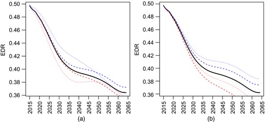
Effects of fertility and net flow on EDR: (a) effect of varying fertility by ±30% ( , baseline;
  , gradual, 30%;
  , instant, 30%;
  , gradual, 30%;
  , instant, 30%); (b) effect of varying LFPR in increments of 15000 (
 , 20000;
  , 35000;
  , 50000;
  , 65000;
  , 80000)
These results are further discussed in the next conclusion section.
9. Discussion and conclusion
In this study, we have used modern FDA methods to project fertility, mortality and LFPR and used these to project two measures of age burden out to 2064. The large contribution of migration to population growth, as well as the gender skew that this is causing, are interesting complicating factors and we have attempted to model these less formally.
Our projections suggest that large increases in the age burden are seemingly inevitable for Hong Kong. There are policy discussions in Hong Kong of how best to increase fertility and to attract migrants to maintain a healthy population structure, yet the ultimate effects of these changes were not well understood. This study quantifies these effects through scenario analyses, where these two drivers are varied by plausible amounts. Our results indicate that varying fertility and migration has a modest cumulative and long-term effect on dependence ratios. The ‘best’ outcomes follow from lower fertility and higher migration regimes. Critical to this conclusion is that we count the young as well as the elderly as dependent. The result for low fertility is not surprising, as fewer babies mean fewer dependants, who are likely not to enter the labour force for at least 20 years. However, reducing fertility is obviously not a sustainable option for Hong Kong, where rates are already very low. They need to maintain a healthy demographic structure to maintain sustainable development into the future.
9.1. Main results
9.1.1. Fertility
Our projections suggest further postponement of childbearing, associated with the growing norm of delayed marriage. Fertility decisions are influenced by many factors. In Hong Kong, the major concerns are the financial burden of housing and forgone salary, and the weight of responsibility (Family Planning Association of Hong Kong, 2014). Public policies promoting childbearing appear to have limited effect on total fertility, probably because they do not address these basic issues adequately.
There is no indication that the TFR will rise in the foreseeable future. Indeed, as low fertility is now the social norm of modern Hong Kong, it has perhaps acquired its own inertia. Our modelling efforts uncovered no useful predictions of total fertility which was, instead, varied exogenously in our projections.
9.1.2. Mortality
Reducing mortality rates mean a longer lifespan, but not necessarily a longer disability-free life. Consequently, we can expect an increasing healthcare burden in the future (Kwok et al., 2017). A natural increase in population has been low for many years and will reduce to 0 in around 2030.
9.1.3. Migration
Hong Kong has received more than 1 million OWPH migrants in the past two decades and newcomers from mainland China will account for an increasing share of annual population growth. The majority are in the working age group and so provide an immediate and steady supply to the labour force. Again, there was no useful prediction of total numbers and we varied this by plausible amounts in our projections.
9.1.4. Gender balance
The proportion of females is increasing systematically, mainly because of a gender skew in OWPHs driven by a gender asymmetry in cross-border marriages. This creates a marriage squeeze for Hong Kong women. There are signs that the reducing economic gap between Hong Kong and mainland China will reduce this asymmetry and that cross-border marriages of Hong Kong women to mainland men are already starting to increase. The effect of increasing gender imbalance on fertility is unclear. Although we have modelled this process, it remains an open question whether every female in Hong Kong can find a partner. Formal marriage is essential for a traditional Chinese culture like Hong Kong's, where birth out of wedlock is still rare (about 6%).
9.1.5. Labour force participation
The main patterns are decreasing rates for the young, increasing rates for the old, increasing rates for females aged 30–50 years off a low base and decreasing rates for males aged 30–50 years off a high base. We address these in turn.
The decreasing rates for the young reflect time spent in higher education. Skills training is important for those eschewing tertiary level education, so that they still have an entry into the productive workforce. Labour participation rates among older adults in Hong Kong are the lowest in the region (Chief Secretary for Administration's Office, 2015) but are strongly increasing. Taken together, the patterns for the old and the young mean that the LFPR age profile is moving to the right, i.e. the labour pool becomes older, partly in response to demographics.
Rates for females are increasing at ages over 30 years, from a historical pattern where rates dropped from the age of 25 years, because of family duties. Although rates are moving in the right direction, the projected increases in the rates for females are only projections and will need pronatalist employment policy support to be realized. Rates for males in the productive years have reduced from 98% to 96%, possibly because of increasing affluence.
9.1.6 Age burden
Our two metrics of age burden, namely the ADR and EDR, treat young and old non-productive people as equally burdensome. It is more common to consider only the burden of the elderly which automatically leads to recommendations of increased fertility. Indeed, the higher the fertility the lower the proportion of elderly will be in the limit. Yet, anyone who has had children knows that they are a cost, as well as a joy.
Thus our results show that increasing fertility will increase the total economic burden (as measured by the ADR or EDR) both in the short and the medium terms. In the very long term, increased fertility means a younger average age but this can mean a higher or lower ADR or EDR, depending on the exact shape of the population and the labour force patterns.
Without doubt, the ADR and EDR are set to deteriorate drastically over the next 50 years, regardless of fertility or migration settings. It is the latter that will have the greatest mitigating effect on the basis of plausible policy changes, though such changes are politically difficult. It is worth noting also that increases in migration from the mainland will not lead to overpopulation but rather to a population equilibrium.
9.2. Some specific policy issues
Since the total population in Hong Kong will peak in around 2030 under current projections, an increased migration quota is a possible response to demographic burdens. However, the migration policy lever might be limited by negative local sentiments if the local carrying capacity is not improved accordingly.
The younger a mainland child is admitted, the easier they can adapt to Hong Kong's education system and local community (Bacon-Shone et al., 2008; Yip and Lee, 2000). A flexible management scheme of the OWPH quota could avoid long waiting times for family reunions and facilitate the supply of labour. Infrastructure needs to be built to remove barriers to settlement so that this human capital can be unleashed into the capacity building of the community.
There are encouraging signs that females and the elderly are increasing their labour force participation. Most advanced countries have already extended their retirement age, supplementing this with flexible working hours, retraining and initiation of some re-employment plans with affordable medical insurance coverage. The challenge for Hong Kong, therefore, will be to support physically and cognitively fit older people to remain or even to return to the workforce.
Pursuing a career and raising children are not necessarily incompatible. Some Organisation for Economic Co-operation and Development countries (e.g. Norway and Sweden) have maintained fertility rates at around 1.8, whereas female participation has shown large increases, going from about 50% to 75% during the period 1975–2015. In France, both the TFR (about 1.7–1.8) and the female LFPR (about 70%) remain at high levels. Koppen (2004) showed that compatibility between work and family life is high in France, where highly educated women are more likely to have a second child than are less educated women. The increase in female labour force participation could generate further gains in income per capita and lessen the acute labour shortage, and the examples of other countries demonstrate that this is achievable. Child care service for local working women in Hong Kong is severely lacking and unaffordable to many.
9.3. Conclusion
The demographic window of opportunity will soon close in Hong Kong, as in many other high income Asian countries, such as Singapore, Taiwan and South Korea. Hong Kong's population growth will slow, the workforce will inevitably shrink and the gender balance will become skewed towards females. Policies that attract outside talent and which promote fertility may slow these trends, but only at the margin. The poor ADR and EDR in 50 years, which is the result of a sharp decline in fertility in the past and consistent mortality decline, remain similar under all plausible scenarios. To tackle the effect of population aging, simple demographic inputs are necessary but just not sufficient.
A highly skilled, educated and sufficiently numerous workforce is vital if Hong Kong seeks to become a successful knowledge-based and service-oriented economy. Hong Kong needs a forward looking, integrated and evidence-based population, education, labour and migration policy to achieve a sustainable and diversified economy. Training and education opportunities should be provided to all the young people of age 15–24 years. Policies targeting specific ages and levels of education, where the effect will be greatest, should be considered. Labour policy should focus on facilitating the participation of women and those in older age groups. Migration should focus on those in the productive ages and reversing the gender skew. A key task will be to tune policy to utilize the human capital from mainland migrants.
Embracing and understanding demographic challenges and economic burdens are among the highest priorities of the Hong Kong Government today. This has largely motivated our analysis, which will also have a bearing on other societies which have undergone a similar rapid demographic transition.
Acknowledgement
The third author was supported by a Hong Kong ‘Strategic public policy research’ grant (SPPR-HKU-12).
