


Summary
Administrative data sets are increasingly used in research because of their excellent coverage and large scale. However, in the UK the use of administrative data on individuals’ earnings, and particularly graduates’ earnings, is novel. Understanding the strengths and weaknesses of such data is important as they are set to be used extensively for research and to inform policy. Here we compare survey-based labour earnings data from the UK's Labour Force Survey (LFS) with UK Government administrative sources of individual level earnings data, focusing separately on young (up to age 32 years) graduates and non-graduates. This type of administrative data set has few sample selection issues and is longitudinal and its large samples mean that the earnings of subpopulations can potentially be studied with low error. Overall we find a similar share of individuals with zero earnings in the LFS and administrative data, but a considerably higher share (conditionally on working) earning below £8000 in the administrative data. The LFS has generally higher earnings right through the distribution, though above the median a large share of the differences can potentially be explained by employee pension contributions. We also find considerably larger gender difference in the survey data. The findings hold for both graduates and non-graduates. These differences are substantively important and suggest different conclusions about the gender wage gap, the graduate earnings premium and the extent of earnings inequality.
1. Introduction
A rich literature has shown the power of administrative tax records to understand better the earnings of subpopulations (e.g. Chetty et al. (2014a, 2014b)). Such data have comprehensive coverage, clearly defined income categories and individual (or household) level data that stretch over significant periods of time. Given these advantages, as discussed in Savage and Burrows (2009), Webber (2009) and Card et al. (2010), there is a growing literature on the application of large-scale administrative data to understand the outcomes from education (see Figlio et al. (2015), Black et al. (2005), Bhuller et al. (2017) and Carneiro et al. (2013) for illustrations of the use of such data). However, although administrative data have been used to good effect to study labour markets in many countries, their use in the UK is in their relative infancy and there has been little work establishing the quality of such data.
Here we build and document a new database that we call the ‘golden sample’ (GS) that links administrative tax records for young (up to age 32 years) individuals to their Student Loan Company (SLC) records. This enables us to investigate the earnings of English graduates. We compare the GS's summary statistics with corresponding results from a well-established government-funded labour market sample survey, the Labour Force Survey (LFS), exploring the relative strengths and weaknesses of both of these sources of data. Such data are set to take a more prominent role in UK policy making in years to come. For example, current estimates of the long-run costs of income contingent student loans in the UK, which require the forecasting of graduates’ earnings several years into the future, are largely based on survey data, and the LFS in particular. The administrative data set that we introduce here is set to be used by the UK Government to investigate these long-run costs, as it provides rich earnings information with long panels with large sample sizes and links to higher education (HE) providers and subject choice that allow detailed breakdowns of the cost of loans by subpopulations. Documenting the differences between, and relative advantages of, the administrative and survey data, particularly for graduates’ earnings, is therefore of great importance for researchers and policy makers. For comparison, we also build a less rich data set of UK-based non-graduates, which we call the ‘silver sample’ (SS), and compare it with non-graduate LFS data.
We compare our administrative data with the LFS, which is a survey that is commonly used to estimate graduate earnings (e.g. Walker and Zhu (2011)) and other labour market measures (e.g. Cribb and Joyce (2015)). Overall we find a similar share of individuals with zero earnings in the LFS and the administrative data, but a considerably higher share (conditionally on working) earning below £8000. The LFS has generally higher earnings right through the distribution, though above the median a large share of the differences can potentially be explained by employee pension contributions. These findings are robust to whether we are looking at graduates or non-graduates.
These differences have implications for future research and public policy. The administrative data sets are the official earnings records for an individual and hence the earnings that are relevant for the loan repayment calculations and for tax receipts. Further, we also believe that the administrative data are more reliable than the LFS, at least conditionally on earnings being greater than £ 8000. However, we find that the high share of individuals earning between £0 and £8000 and in particular the lack of gender differences in the lower part of the distribution in the administrative data are not just inconsistent with the LFS but also with the Family Resources Survey, which is another commonly used survey for studying earnings. There are various potential explanations for this, including sample selection or non-response bias that results in low earners being under-represented, measurement error, in particular annualizing earnings from sometimes shorter periods and the treatment of those with variable income, and the inclusion of sources of income other than earned income, such as salary sacrifice pension contributions. Alternatively, the administrative data may suffer from under-reporting of income to avoid paying tax or to qualify for benefits, and also has issues that are caused by the inclusion of all English-domiciled borrowers rather than graduates. All these issues are discussed in more detail below, when we use the data to measure the gender wage gap, the graduate wage premium and earnings inequality among graduates and non-graduates. We show how important conclusions that are made about the economic advantages or otherwise of taking a degree differ, depending on which source of data is used. This paper serves to improve our understanding of the different features of the two sources of data and, although we conclude that the administrative data do indeed have considerable advantages over the survey data, we also highlight limitations that need to be understood by researchers if such data are to be used to best effect.
The rest of the paper is laid out as follows. In Section 2 we review the literature and in Section 3 we detail the linkage of administrative data. In Section 4 we discuss the UK LFS and summarize the key differences between the sources of data. Section 5 compares earnings distributions of LFS graduates versus the GS, LFS non-graduates versus the ‘non-HE’ sample (a corrected version of the SS) and the overall LFS population versus the combined GS and SS populations. Section 6 makes applied comparisons, investigating differences in the gender wage gap, the graduates-to-non-graduates earnings ratio and earnings inequality, and Section 7 concludes. An on-line appendix contains various additional results that are referred to in this paper.
The programs that were used to analyse the data can be obtained from
https://dbpia.nl.go.kr/jrsssa/issue/
2. Literature
This paper builds on a significant literature (e.g. Bound et al. (2001), Abowd and Stinson (2013) and Koijen et al. (2015)) which has discussed the problems of using sample surveys, particularly in relation to measuring income, comparing their results with some administrative data. There are also specific data collection issues in the LFS. Skinner et al. (2002), for example, have found significant discrepancies in earnings estimates for the low paid by using different ways to calculate hourly pay in the LFS. Traditionally, hourly pay in the LFS was calculated by using weekly pay received divided by usual working hours. More recently, the LFS has included an hourly rate of pay variable. Skinner et al. (2002) concluded that this variable has less measurement error but is missing for a significant proportion of the sample. Imputing earnings for those with missing data on the hourly rate of pay variable leads to substantially reduced estimates of the proportion who are low paid. Bound et al. (2001) discussed sources of error in earnings surveys, concluding that self-reported annual earnings tend to have less error than disaggregated measures, such as hourly or weekly earnings (see also Duncan and Hill (1985)). Bound et al. (2001) also found evidence that survey errors are mean reverting. There was mixed evidence on whether graduates or individuals with more human capital were more likely to report their earnings with error, though some studies that have compared survey measures with administrative records have found a positive correlation between true earnings and error in earnings (e.g. Rodgers et al. (1993)). Bound et al. (2001) found limited evidence that respondents with very high earnings tend to under-report their earnings and those with very low earnings overreport theirs, rejecting the theory of ‘social desirability bias’ where individuals report with bias to appear less different. However, they did find non-negligible measurement error in measures of schooling and highest education level: individuals can misreport or misremember their years of schooling or highest level of qualification. This measurement error in reported schooling levels will in turn cause measurement error in estimates of earnings differences by level of education, even if individuals report their earnings correctly.
A review by Moore et al. (2000) that focused on sources of error in earnings measures in official surveys suggested a wide range of sources of bias. Non-response is an issue. Respondents may not completely understand the different definitions of earnings being used (e.g. in the LFS they are asked for earnings both ‘before deductions’ and net pay ‘after deductions’). Questions may not be precise about the inclusion of pension contributions and child care allowances, and individuals may have recall problems depending on the period being asked about. Although it is well known that earnings data collected with a single question are subject to extensive measurement error (e.g. Micklewright and Schnepf (2010)), even when more complex survey designs are used it remains a challenge to design high quality instruments for measuring earnings in surveys, particularly if household members are being asked to report on the earnings of others (this is so with the LFS: in practice we actually find that removing proxy responses makes little difference to our conclusions). Indeed previous work has identified differences in earnings estimates across a number of survey-based sources. For example, comparing UK individual survey data on earned income (from the Family Expenditure Survey and the General Household Panel Survey) with surveys of businesses (the Annual Survey of Hours and Earnings, which is based on a 1% sample of employee jobs taken from Her Majesty's Revenue and Customs (HMRC) Pay As You Earn (PAYE) records, with information on earnings and hours obtained from employers) have tended to find that the former underestimate the earnings of respondents compared with the latter (Atkinson et al., 1981, 1982; Devereux and Hart, 2010). It should be noted that, although the Annual Survey of Hours and Earnings does sample from HMRC tax records, it is based on a survey of employers only and so does not include self-assessed earnings nor those not paid in the reference week. It is also still based on a survey methodology and suffers from non-response, meaning that it is not directly comparable with our work.
This paper contributes to this literature in several ways. First, the paper compares the distribution of earnings in the administrative data with the LFS and highlights the potential limitations of both data sets, which is an issue of increasing relevance as administrative data sources start to become more readily available for policy makers. Second, it provides evidence on the level and variation of UK graduate earnings by using this new high quality data source (Naylor et al., 2016; Walker and Zhu, 2011). Third, it highlights the rich potential of this data set for understanding inequality in earnings, adding to the large body of work on this issue (Cunha and Heckman (2016) have provided a comprehensive summary). Fourth, it provides UK evidence on the gender wage gap particularly among graduates, again building on previous UK empirical work which has often relied on survey data and the LFS specifically (Machin and Puhani, 2003; Chevalier, 2007).
3. Our administrative databases
3.1. The golden sample
The GS is a database that we built, using national insurance numbers to hard-link three data sets: data from the SLC and PAYE and self-assessment (SA) databases from HMRC. This provides us with a large longitudinal database on UK earnings for individuals domiciled in England on application to HE, who received loans from the SLC.
The two HMRC data sets arise because the UK has two types of income tax forms. The significant majority of taxpayers use the PAYE system, which is operated by employers who withhold income and other employment taxes and report the earnings and deductions made to HMRC. This means that the majority of UK citizens do not themselves file tax forms; Pope and Roantree (2014) reported that around 90% of UK income tax is collected through the PAYE system. For those with more complicated tax affairs (e.g. high incomes, self-employed, owning a business, having significant investment accounts or being in a professional partnership) HMRC require them to file a set of SA forms. Individual taxpayers can also opt to submit SA forms.
The UK runs an individual tax filing system with no option to file as a household. Thus UK administrative data will be good for studying individuals’ earnings but, unlike in the USA (e.g. Guvenen et al. (2014)), not good for household earnings. HMRC do have address information which would allow the fuzzy linkage into households, but we do not have access to this information. We therefore focus on individual rather than household earnings.
3.1.1. Earnings data
Our focus is on earned labour income, so we defined this as the sum of employment income, profits from partnerships and profits from self-employment declared to HMRC. Clearly some aspects of the returns from a partnership are due to the capital risk that a partner is exposed to, but we cannot break that component out here and so take profits from partnerships as earnings.
The SA databases also contain information on trust income, profits on share transactions, profits from land and property, UK dividends, pension income, life policy gains, ‘other’ income, bank and building society interest and total income, all of which we exclude from earned income as they measure non-employment income. We wanted to include foreign income from employment and savings, but the calculation involved various delicate deductions, so we excluded it.
We do not make a record of any deductions that taxpayers make, e.g. capital losses on investments, nor of any tax-free allowances that individuals may have. We also do not account for employers’ and employees’ tax-free pension contributions as labour earnings as UK tax forms record only pension income and not pension contributions.
When we have both PAYE and SA earnings we use the SA data, as HMRC regard the SA records as definitive (noting that an SA form will include PAYE income). If an individual has no reported earnings then we take their earnings as 0. This is likely to miss some earnings for very low earners who do not have to return a PAYE form and who may not be asked to complete an SA form (although note that they have a legal responsibility to report this income). All earnings are converted into October 2012 prices by using the consumer price index.
3.1.2. Student Loan Company data
The SLC has offered income contingent loans to all UK-domiciled HE students since 1998. The take-up rate among eligible students during this period is around 85–90% overall, which is a rate that has remained relatively stable (authors’ own calculations based on overall student numbers from the SLC ‘Student support for higher education in England’ archived series). Not all individuals receiving a loan from the SLC will be studying for first degrees, as individuals can access loans for foundation degrees, Higher National Diplomas and lower undergraduate qualifications. The data set that we received from the SLC does not have any indicators to split individuals into these different groups. We observe the final degree for which an individual qualifies for a loan. So, for example, for someone attending an HE institution for a term before dropping out and restarting at a different institution sometime in the future, only their second degree is observed so long as they borrowed again (though the date that they started in HE is the first-degree start date).
The data set includes only individuals who borrowed from the English part of the SLC—meaning that they were domiciled in England on application—between 1998 and 2010—and covers around 2.6 million former borrowers who are qualified to be in repayment, which happens in April of the year after they leave HE. We have no data on those who are still in HE and have insufficient earnings to qualify them for repayment, which results in a decline in our cohort sizes for more recent student cohorts (Table 1). Note that we observe only borrowers and not whether individuals graduate, resulting in individuals who borrow from the SLC but subsequently drop out being inaccurately defined as graduates (throughout, we use the terms ‘borrowers’ and ‘graduates’ interchangeably). During this period the dropout rate from UK universities for those who enrol was around one in 10, including mature entrants (taken from Higher Education Statistics Agency performance indicators data series, where the Higher Education Statistics Agency measures drop out by those who attended for at least 90 days before dropping out).
Number of GS (10% sample of loan database) borrowers and tax data in 2011–2012†
| Cohort | Results for all | Results for males | Results for females | |||||||||
|---|---|---|---|---|---|---|---|---|---|---|---|---|
| GS | PAYE | SA | Either | GS | PAYE | SA | Either | GS | PAYE | SA | Either | |
| 1998 | 14487 | 11646 | 2310 | 12226 | 6927 | 5528 | 1351 | 5875 | 7560 | 6118 | 959 | 6351 |
| 1999 | 22621 | 18410 | 3447 | 19354 | 10590 | 8529 | 1912 | 9063 | 12031 | 9881 | 1535 | 10291 |
| 2000 | 23506 | 19214 | 3425 | 20176 | 10853 | 8761 | 1908 | 9322 | 12653 | 10453 | 1517 | 10854 |
| 2001 | 23924 | 19921 | 3108 | 20818 | 11025 | 9060 | 1759 | 9625 | 12899 | 10861 | 1349 | 11193 |
| 2002 | 23891 | 20104 | 2814 | 20906 | 11060 | 9156 | 1576 | 9642 | 12831 | 10948 | 1238 | 11264 |
| 2003 | 23972 | 20387 | 2447 | 21097 | 11024 | 9315 | 1314 | 9726 | 12948 | 11072 | 1133 | 11371 |
| 2004 | 23577 | 20367 | 2266 | 20997 | 10767 | 9163 | 1251 | 9526 | 12810 | 11204 | 1015 | 11471 |
| 2005 | 25103 | 21800 | 2085 | 22397 | 11439 | 9822 | 1141 | 10183 | 13664 | 11978 | 944 | 12214 |
| 2006 | 25383 | 22149 | 1864 | 22589 | 11340 | 9749 | 992 | 10024 | 14043 | 12400 | 872 | 12565 |
| 2007 | 25352 | 22303 | 1527 | 22694 | 11292 | 9746 | 774 | 9981 | 14060 | 12557 | 753 | 12713 |
| 2008 | 20847 | 18154 | 1039 | 18430 | 8990 | 7704 | 531 | 7872 | 11857 | 10450 | 508 | 10558 |
| 2009 | 6510 | 5386 | 426 | 5485 | 3029 | 2452 | 215 | 2509 | 3481 | 2934 | 211 | 2976 |
| 2010 | 2993 | 2477 | 152 | 2511 | 1334 | 1082 | 72 | 1101 | 1659 | 1395 | 80 | 1410 |
| 2011 | 851 | 721 | 724 | 360 | 291 | 294 | 491 | 430 | 430 | |||
| All | 263000 | 223000 | 27000 | 230000 | 120000 | 100000 | 15000 | 105000 | 143000 | 123000 | 12000 | 126000 |
PAYE and SA denote databases. Either denotes being in either PAYE or SA or both. Cohort denotes the first year that the borrower received a loan from the SLC.
3.1.3. Linking the administrative data sets
Primarily because of computational limitations, HMRC have allowed us to link 10% of individuals in the SLC data to the tax data, with the 10% selected on the basis of two digits within each individuals’ randomly allocated national insurance number. HMRC use the same 10% for much of their own analysis. Because we have the full sample of borrowers, our 10% sample includes the small fraction of individuals who never file a return with HMRC.
We call this 10% matched sample the GS. We have up to 11 tax years (note that the tax year runs from April 6th to April 5th each year) in the data set for each individual, from 2002–2003 to 2012–2013, although the majority of our focus here is on the 1998–2003 cohorts in the period from 2008–2009 to 2012–2013 to give individuals sufficient time to complete their degrees and to enter the labour market after starting their HE course. Once submitted to HMRC, UK tax forms are highly confidential and access to them is restricted by Parliamentary statutes. We have been given access to an anonymized version of the data and our work was carried out in a highly secure data enclave within an HMRC facility. All outputs are checked by officials to ensure that they cannot be disclosive of any individual's information.
The matching is a hard link based on the individuals’ national insurance number, which is available in both data sets and the quality of which is checked many times (for more detailed information on this see Britton et al. (2015)). These data therefore do not suffer from the weaknesses of some other linked administrative data sets; for example Chetty et al. (2014a) reported linkage rates close to 90% by using fuzzy matching, based on date of birth, state of birth, names and gender, between school reports and tax records and just under 98% for matching parents to children (although it should be noted that Chetty et al. (2014a) did have considerably larger sample sizes).
A drawback is that, when former students become non-resident for UK tax purposes, HMRC may lose contact with them and generally will record earnings from only UK sources as these are their UK taxable earnings. We shall express the earnings of such students as 0 in our reports if HMRC records it as 0, which clearly may underestimate their true earnings.
3.1.4. Basic summaries of the golden sample
The GS has 263052 members, covering cohorts from 1998 to 2011. We focus on the tax years from 2008–2009 to 2012–2013. It should be noted that this was a financially difficult period. The GS is detailed for 2011–2012 in Table 1. There are around 24000 students in each cohort, with the smaller 1998 figure reflecting slow uptake of the new income contingent student loans and the decline at the end reflecting the fact that individuals have not entered repayment (i.e. left HE) by 2011–2012. The student numbers align with Higher Education Statistics Agency statistics for 2007–2008, which state that around 325000 UK-domiciled students were studying in England. Our 10% sample is 25000 students in this year, meaning a cohort size of around 250000 borrowers. Around 15% of the English students do not borrow (taking us to 295000), whereas the remaining students would be non-English UK students studying in England.
Each individual potentially has an SA and a PAYE tax record in each tax year but may have neither. By construction, we can state that if they have neither an SA nor a PAYE record then they have no UK tax return at all—note that, unlike in the USA, in the UK it is not legally necessary to file a tax form if your income is indeed 0, although it is required for any amount above 0. We shall record such non-filers as having zero earnings. We end up with the GS for whom we have earnings data from the PAYE database, the SA database or both.
Table 1 gives the breakdown of different types of tax forms for 2011–2012 by gender and cohort. It shows that a significant majority of borrowers are female for all cohorts, reflecting greater HE participation among women. In more recent cohorts there are very little SA data since it is higher earners and the self-employed who are more likely to use SA, both of which become more likely with age. There are some people, mostly self-employed, who appear only in the SA data (for example, in 1998 of the 14487 individuals in the GS, 12226 have tax records for that year and 1730 had only SA records—this is equal to 11646 + 2310 – 12226) and a considerably higher rate of SA for males.
Table 2 shows the percentage of individuals who filed no tax form at all during 2011–2012, and the share with no and low earnings, by cohort (with the median age of the cohort indicated). The columns are cumulative, so the share with earnings of less than £8000 includes those with zero earnings and those with no filed tax form. For those with no form, we assume that the individual has zero taxable income in the UK. The rate of not filing initially decreases moving up through the cohorts, but then increases. There is little gender difference in the not-filing-rate, even as the cohort reaches their early 30s, which is surprising given evidence on the unequal split of child care responsibilities—one possible explanation might be predominantly female individuals paying national insurance contributions even when they have zero earnings to preserve pension benefits in later life, although we do not attempt to quantify this here. There is a sizable group of people in the databases with returns of zero income (given by subtracting the share with no form from the share with earnings of £0; for example, for the 1998 cohort, 2.7% of women filed returns of zero earnings). This might arise, for example, from employers filing PAYE returns for former employees. Again there is very little difference by gender.
GS for 2011–2012: percentages of individuals with no filed income form and percentages with no or low earnings†
| Median age (years) | Cohort | % no tax form | % earnings = (or no form) £ 0 | % earnings < £ 8000(includes 0s and missing values) | ||||||
|---|---|---|---|---|---|---|---|---|---|---|
| All | Males | Females | All | Males | Females | All | Males | Females | ||
| 31 | 1998 | 13.0 | 12.6 | 13.3 | 15.6 | 15.2 | 16.0 | 27.3 | 26.7 | 27.9 |
| 30 | 1999 | 11.7 | 11.4 | 11.9 | 14.4 | 14.4 | 14.5 | 26.2 | 25.7 | 26.7 |
| 29 | 2000 | 11.4 | 11.2 | 11.5 | 14.2 | 14.1 | 14.2 | 26.1 | 25.7 | 26.5 |
| 28 | 2001 | 10.1 | 9.9 | 10.3 | 13.0 | 12.7 | 13.2 | 25.0 | 24.5 | 25.5 |
| 27 | 2002 | 9.6 | 9.9 | 9.3 | 12.5 | 12.8 | 12.2 | 25.3 | 25.5 | 25.0 |
| 26 | 2003 | 9.0 | 8.9 | 9.0 | 12.0 | 11.8 | 12.2 | 25.8 | 25.4 | 26.1 |
| 25 | 2004 | 8.0 | 8.3 | 7.7 | 10.9 | 11.5 | 10.5 | 25.9 | 26.8 | 25.2 |
| 24 | 2005 | 7.5 | 7.4 | 7.5 | 10.8 | 11.0 | 10.6 | 29.1 | 30.3 | 28.2 |
| 23 | 2006 | 7.5 | 7.8 | 7.2 | 11.0 | 11.6 | 10.5 | 34.3 | 36.3 | 32.6 |
| 22 | 2007 | 7.0 | 7.8 | 6.3 | 10.5 | 11.6 | 9.6 | 43.2 | 45.1 | 41.8 |
| 21 | 2008 | 8.4 | 9.1 | 7.8 | 11.6 | 12.4 | 11.0 | 61.6 | 63.2 | 60.4 |
| 21 | 2009 | 10.9 | 11.6 | 10.4 | 15.8 | 17.2 | 14.5 | 61.1 | 64.6 | 58.0 |
| 20 | 2010 | 11.0 | 12.0 | 10.2 | 16.1 | 17.5 | 15.0 | 67.9 | 72.0 | 64.6 |
| 18 | 2011 | 10.1 | 13.1 | 7.9 | 14.9 | 18.3 | 12.4 | 90.6 | 90.6 | 90.6 |
Columns are cumulative so the share with earnings less than £8000 includes those with earnings £ 0 and those with no form. Median age does not decrease by 1 each year in the GS because of small sample sizes and variation in the ages of HE leavers (since individuals only enter our data set once they have left HE).
The rate of borrowers with zero earnings appears to be high, accounting for over 14% of individuals aged around 30 years. However, this figure is comparable with SLC official statistics (which are not perfectly equivalent, as they include European Union borrowers). These show that, of the 2001 cohort in 2013–2014 (as close to the equivalent for the 1999 cohort in 2011–2012 as we could achieve), 9% still have debt but have no employment. Approximately 1.4% of individuals have had their loans written off because of death, disability or bankruptcy and 37% have cleared their debts. Some individuals in each of the latter groups will have zero earnings but would not be incorporated in the 9% figure. If all of those with debt written off because of death, disability or bankruptcy were on zero earnings, that would be 10.4% of borrowers and, if just 7% of those with cleared debts were also on zero earnings, that would take us to around 13%.
The remaining difference can most likely be explained by individuals moving abroad. Table 3 summarizes some additional SLC information on this. This shows that around 1% of the 1999 cohort were abroad and in repayment in 2011–2012. These data are incomplete, as the SLC does not continue to track individuals’ country of residence once they are out of repayment—we therefore also show figures for individuals who have been abroad at any point (which includes those currently abroad). This is around 4% for the 1999 cohort in 2011–2012. Table 3 also shows the share of individuals with no and low (less than £8000) earnings. Around 80% of those currently abroad have earnings in the UK below £8000, whereas more than half of those ever abroad do. This shows that some individuals still file while they are abroad, but it also suggests that more than 1% of individuals are abroad at any given time. Combining this with the 13% figure above, this therefore moves us close to SLC official records. The UK Department for Education has also started to use HMRC administrative data on earnings separately (with some notable differences; they do not yet use SA data, and they cannot hard-link data sets to identify graduates by using national insurance numbers) and their calculations suggest a similar proportion of graduates with zero earnings.
SLC in repayment and living abroad data in 2011–2012†
| Cohort | % abroad | % been abroad | Of those abroad | Of those been abroad | ||
|---|---|---|---|---|---|---|
| Earnings =£0 | Earnings <£8000 | Earnings =£0 | Earnings <£8000 | |||
| 1998 | 1.0 | 4.4 | 73.2 | 40.8 | 50.6 | |
| 1999 | 1.1 | 4.2 | 69.8 | 86.8 | 42.7 | 52.2 |
| 2000 | 1.2 | 4.0 | 61.7 | 80.7 | 42.0 | 53.9 |
| 2001 | 1.2 | 4.1 | 66.2 | 78.5 | 42.5 | 52.2 |
| 2002 | 1.3 | 3.8 | 58.4 | 78.1 | 39.5 | 52.1 |
| 2003 | 1.4 | 3.7 | 57.0 | 73.8 | 40.8 | 55.1 |
| 2004 | 1.4 | 3.8 | 47.7 | 71.8 | 36.4 | 54.9 |
| 2005 | 1.4 | 3.4 | 55.9 | 82.6 | 39.3 | 61.9 |
| 2006 | 1.4 | 2.6 | 51.2 | 85.3 | 43.1 | 73.5 |
| 2007 | 1.4 | 1.9 | 43.8 | 86.0 | 44.0 | 82.9 |
| 2008 | 0.6 | 0.7 | 34.1 | 35.3 | ||
Abroad is an indicator for being overseas and in repayment according to SLC records. Been abroad is an indicator for abroad and in repayment or have been in this state at some point in the past. Figures are excluded where the implied sample sizes are too small.
Table 2 also records the percentage of borrowers with incomes below £ 8000. This level was selected since it is approximately the level of earnings at which individuals start to pay national insurance contributions and income tax (Pope and Roantree, 2014), meaning that the administrative data are more likely to be reliable above this level. Around a quarter of borrowers earn less than £8000 around their late 20s and early 30s, with again only a relatively small difference between genders. This finding is stark, and we return to it below.
One concern is under-reporting of earnings, which is an issue that might be a particular problem for the self-employed, for whom it is easier to move income into other forms as there is no employer-based filing which can be used to verify the income independently. Indeed Her Majesty's Revenue and Customs (2014) have estimated the amount of uncollected tax that is caused by the under-reporting of income, finding a tax gap of around 17% for self-assessed taxes (with around 25% of SA taxpayers under-reporting their earnings) and 1.5% for PAYE taxes. Since the vast majority of our data comes from PAYE sources, and the majority of those with SA reports also have most of their earnings recorded through employer-based PAYE records (i.e. the ‘P60’ form), the main vulnerability of the tax data is therefore to under-reporting from the fully or partially self-employed.
Table 4 quantifies the degree of self-employment in this data set, showing how it varies with cohort and gender. Around 10% of our sample are either fully or partially self-employed. We have not made any correction to the raw HMRC data in our analysis to take this under-reporting into account, though we would obviously expect this to bias our estimates for this group downwards. The proportion of borrowers who have earnings only from self-employment is roughly 1–3%, clearly increasing with age and with a higher rate for men than women. Of these, around 35% of men report labour earnings of below £8000, whereas the equivalent figure for women is almost 60%. A higher rate of partial self-employment is recorded, again with males having higher incidence than females. Among these individuals, women again have a considerably higher chance of having low earnings. We refer to this when considering the high incidence of low earnings in the tax data in Section 5.
GS self-employment: the cohort who are only partially self-employed (not those fully self-employed) and those entirely self-employed†
| Median age (years) | Cohort | Results for only partly self-employed | Results for entirely self-employed | ||||||||||
|---|---|---|---|---|---|---|---|---|---|---|---|---|---|
| Of all (%) | Of self-employed part:% earnings < £ 8000 | Of all (%) | Of self-employed only:% earnings < £ 8000 | ||||||||||
| All | Males | Females | All | Males | Females | All | Males | Females | All | Males | Females | ||
| 31 | 1998 | 6.4 | 7.1 | 5.7 | 33.4 | 27.1 | 40.7 | 3.6 | 4.4 | 2.8 | 44.9 | 35.4 | 58.8 |
| 30 | 1999 | 6.5 | 7.3 | 5.8 | 34.6 | 30.3 | 39.3 | 3.8 | 4.5 | 3.1 | 46.4 | 39.4 | 55.3 |
| 29 | 2000 | 6.6 | 7.5 | 5.8 | 33.8 | 31.7 | 36.1 | 3.7 | 4.6 | 2.9 | 46.7 | 42.9 | 51.9 |
| 28 | 2001 | 6.2 | 7.5 | 5.1 | 34.3 | 31.7 | 37.5 | 3.5 | 4.7 | 2.5 | 47.6 | 43.4 | 54.4 |
| 27 | 2002 | 5.8 | 6.9 | 5.0 | 35.9 | 35.5 | 36.3 | 3.3 | 4.3 | 2.4 | 47.2 | 46.3 | 48.7 |
| 26 | 2003 | 5.4 | 6.1 | 4.8 | 37.9 | 33.9 | 42.1 | 3.0 | 3.6 | 2.5 | 52.1 | 46.6 | 58.9 |
| 25 | 2004 | 5.2 | 6.2 | 4.3 | 38.8 | 36.2 | 41.9 | 2.8 | 3.6 | 2.1 | 51.7 | 47.7 | 57.6 |
| 24 | 2005 | 4.9 | 5.9 | 4.1 | 41.3 | 41.5 | 41.1 | 2.6 | 3.3 | 2.0 | 58.3 | 55.3 | 62.6 |
| 23 | 2006 | 4.3 | 5.1 | 3.7 | 47.6 | 46.6 | 48.8 | 2.2 | 3.0 | 1.5 | 63.1 | 59.7 | 68.5 |
| 22 | 2007 | 3.8 | 4.4 | 3.4 | 54.7 | 50.7 | 58.8 | 1.9 | 2.5 | 1.5 | 68.2 | 61.2 | 77.7 |
| 21 | 2008 | 3.1 | 3.6 | 2.7 | 67.9 | 68.3 | 67.5 | 1.7 | 2.4 | 1.2 | 78.1 | 78.0 | 78.1 |
| 21 | 2009 | 3.4 | 4.0 | 3.0 | 62.5 | 63.3 | 61.5 | 1.8 | 2.2 | 1.4 | 85.2 | 86.4 | 83.7 |
| 20 | 2010 | 2.8 | 3.4 | 2.4 | 61.9 | 1.3 | 87.5 | ||||||
Also given are the corresponding percentages who have low earnings. Earnings are all earnings from work, not just from the self-employed part. Results are for the 2011–2012 tax year. See the footnote to Table 2 to explain the pattern for median age.
3.2. The silver sample
The HMRC and SLC linking also yields a sample of people who did not take out loans from the English part of the SLC. The significant majority of these UK people are non-graduates. This database is called the SS.
The SS is built by taking the 10% national insurance number sample (which, as described above, is a random 10% sample of the population) in the tax data and removing all those who appear in the SLC database. Specifically, this means that the SS consists of anybody who appears at any point in the PAYE or SA tax data between 2008–2009 and 2012–2013 inclusively, is in the 10% national insurance number sample and does not appear in the SLC data set (meaning that they did not borrow to go to university). For each person in this population we know their age, gender and earnings (including type of earnings) only. Then for each cohort and gender we have sampled this new population to produce a database with the same age profile as in the SLC database. This results in a large database which the HMRC systems have difficulty coping with. We therefore randomly select a subset of the SS, keeping approximately two members of the SS for every one in the GS, which roughly halved the overall size of the SS.
Summaries of the characteristics of the SS are given in Table A1 in the on-line appendix A. There are more men in the SS, reflecting the fact that there are more women in the GS, and the rate of SA is lower in the SS than in the GS (for example in 1999 the GS SA rate is about 15%, whereas for the SS it is about 11%). Table 5 shows that the rate of low pay in the SS is roughly twice as high as for the GS, with 45% of non-graduates with earnings below £8000, compared with 25% of graduates. There is also more of a gender difference than in the GS, with around 50% of females in their early 30s earning below £ 8000 in the SS, compared with 43% of males.
3.2.1. Correcting the silver sample
There are three major issues with the SS (that do not apply to the GS). First, it misses people who have no tax record at all in either of the PAYE or the SA data sets from 2008–2009 to 2012–2013. Second, immigrants entering the country and being assigned a national insurance number will be included and are (at least in principle) also included in the LFS. A problem is created if the individual is not in the country for the entire 5-year period. For example, an individual who enters the country in 2012–2013 would be recorded as having no tax form and hence zero earnings in each of the other years. Third, the SS includes graduates from England who did not borrow (around 15% of English graduates) as well as graduates (and non-graduates) from Scotland, Wales and Northern Ireland.
SS database for 2011–2012: percentages with no filed income tax form and percentages with no and low earnings†
| Median age (years) | Cohort | % no tax form | % earnings = £ 0(or no form) | % earnings < £ 8000(includes 0s and missing values) | ||||||
|---|---|---|---|---|---|---|---|---|---|---|
| All | Males | Females | All | Males | Females | All | Males | Females | ||
| 31 | 1998 | 22.1 | 21.5 | 23.0 | 27.3 | 26.7 | 27.9 | 46.3 | 43.3 | 49.9 |
| 30 | 1999 | 22.6 | 21.3 | 24.2 | 27.7 | 26.6 | 29.0 | 47.5 | 43.8 | 51.9 |
| 29 | 2000 | 23.5 | 21.8 | 25.5 | 28.5 | 27.0 | 30.4 | 48.8 | 45.2 | 53.2 |
| 28 | 2001 | 24.3 | 22.4 | 26.5 | 29.1 | 27.6 | 31.0 | 49.7 | 46.1 | 54.0 |
| 27 | 2002 | 24.8 | 23.1 | 26.8 | 29.7 | 28.3 | 31.4 | 51.2 | 47.9 | 55.1 |
| 26 | 2003 | 25.0 | 23.2 | 27.2 | 29.9 | 28.2 | 31.9 | 51.9 | 48.5 | 55.8 |
| 25 | 2004 | 24.9 | 22.7 | 27.5 | 30.1 | 28.1 | 32.5 | 52.9 | 49.8 | 56.6 |
| 24 | 2005 | 24.2 | 21.8 | 27.0 | 29.3 | 27.3 | 31.7 | 53.8 | 51.2 | 56.9 |
| 23 | 2006 | 23.7 | 21.4 | 26.4 | 29.0 | 26.9 | 31.4 | 55.8 | 53.4 | 58.6 |
| 22 | 2007 | 22.8 | 20.3 | 25.6 | 28.2 | 25.9 | 30.9 | 58.6 | 55.7 | 61.9 |
| 21 | 2008 | 21.6 | 19.4 | 24.1 | 27.8 | 25.4 | 30.5 | 61.6 | 59.0 | 64.5 |
| 21 | 2009 | 20.4 | 19.5 | 21.3 | 26.4 | 25.6 | 27.3 | 64.2 | 62.0 | 66.7 |
| 20 | 2010 | 18.4 | 17.1 | 19.9 | 24.4 | 23.1 | 25.8 | 68.8 | 66.0 | 71.8 |
Median age does not decrease by 1 each year in the SS because the age distribution is matched exactly to the GS (see the footnote to Table 2).
For the first two of these issues, there is little that can be done, since Table 2 shows that a high share of graduates have no tax form, so omitting everybody with no form would dramatically underestimate the share with no earnings. Consequently, we focus much of our later analysis on those with positive earnings only. This resolves the issue with no form and considerably reduces the problem with immigration (it does not completely remove it, however, as immigrants may file a form despite only being present in the country for a fraction of the tax year).
We can correct the third issue by effectively reweighting the earnings distribution of the SS on the basis of the share of graduates whom we believe are in the sample. The result is called the non-HE sample. Let FS(y)=Pr(Y⩽y) be the distribution function of SS earnings Y for a specific cohort and gender. FHE will be the corresponding result for the subset that went into HE and FnonHE is the result for the others. We write ω as the proportion of graduates in the SS; then, by construction,
We now make the assumption that ; then FHE(y)=FG(y) where FG is the distribution function from the GS. This says that the distribution of earnings of the graduates in the SS matches the distribution of earnings in the GS—i.e. the GS well represents all graduates, not just English borrowers. It is important to note that FG is likely to underestimate earnings for English graduates who do not borrow as we might expect this group to come from wealthy families and subsequently to have higher-than-average earnings themselves, but it is difficult to quantify this underestimation (especially as there are other reasons why people may not borrow that might not be positively correlated with subsequent earnings, such as debt aversion).
Under these assumptions, for ,
Since we can estimate FS and FG from the data, we simply need ω to make this correction. Using a combination of data from the Office for National Statistics, government records and SLC data we estimate that ω is equal to around 0.14 for men and 0.21 for women (see the on-line appendix B).
Around a half of these are non-borrowers from England and the rest are all of the graduates from Scotland, Wales and Northern Ireland. Hence the SS will typically overestimate the distribution of earnings for non-graduates, as HE graduates are much more likely to be very high earners than are non-HE people, yielding a large bias if we use it to learn about the upper tail or mean of earnings for non-graduates. However, at the centre of the distribution and in the left-hand tail it is likely to be a good approximation. It should be more accurate for men than for women because the estimated share of graduates in the SS is lower for men than for women.
4. The Labour Force Survey
The LFS has a rolling five-wave design, with 20% of the overall sample replaced with new respondents each quarter. Individuals are surveyed for five consecutive quarters, meaning that five waves of data may be available for one person with the first and fifth waves 1 year apart. Earnings questions appear only in waves 1 and 5. Many people will take the survey but, as is often the case, not provide information on earnings while answering other questions.
Table 6 shows the sample sizes for the LFS between April 2011 and March 2012 (i.e. quarters 2–4 from 2011 and quarter 1 from 2012) for different ages which are the closest match to SLC cohort, by gender and graduate status. The latter is determined from the ‘highest qualification’ question in the LFS, which we choose to align as closely to the HMRC data as possible, meaning that we include all courses that are eligible for student loans (in practice our definition also aligns closely with Walker and Zhu (2011)). Because of the lack of more information on HE, cohorts are assigned to individuals on the basis of their age on August 31st in a given year, which we observe in the LFS special licence access data set. For example, individuals who were 18 years old on September 1st, 1998, are assigned to the 1998 cohort. We focus on individuals who are domiciled in England at the point of survey (rather than on the point of application to HE) and we have included proxy earnings responses, where individuals complete the earnings questions on behalf of a family member (although previous work (Wilkinson, 1998) has suggested that proxy earnings might underestimate true earnings, our findings are not sensitive to this decision).
LFS unweighted samples sizes in England in 2011–2012: number of employment and earnings answers by ages which are the closest match to the SLC cohort and gender†
| Cohort | Results for graduates | Results for non-graduates | ||||||
|---|---|---|---|---|---|---|---|---|
| Number of employment answers | Number of earnings answers | Number of employment answers | Number of earnings answers | |||||
| Males | Females | Males | Females | Males | Females | Males | Females | |
| 1998 | 852 | 1170 | 184 | 261 | 1091 | 1228 | 219 | 221 |
| 1999 | 876 | 1109 | 192 | 253 | 1154 | 1197 | 225 | 204 |
| 2000 | 909 | 1113 | 206 | 248 | 1258 | 1231 | 242 | 200 |
| 2001 | 765 | 1021 | 165 | 218 | 1160 | 1232 | 211 | 202 |
| 2002 | 702 | 1028 | 136 | 206 | 1092 | 1181 | 230 | 203 |
| 2003 | 826 | 927 | 168 | 195 | 1073 | 1144 | 201 | 197 |
| 2004 | 779 | 962 | 156 | 209 | 1038 | 1113 | 213 | 180 |
| 2005 | 785 | 865 | 135 | 160 | 1009 | 1283 | 171 | 218 |
| 2006 | 694 | 851 | 123 | 165 | 1105 | 1221 | 199 | 161 |
| 2007 | 692 | 820 | 108 | 146 | 1045 | 1277 | 175 | 195 |
| 2008 | 659 | 715 | 98 | 109 | 1215 | 1235 | 182 | 207 |
| All | 8539 | 10581 | 1671 | 2170 | 12240 | 13342 | 2268 | 2188 |
The earnings answers are the number of individuals giving positive earnings answers. This question is available in only waves 1 and 5 in the LFS but is still subject to high rates of non-response. Individuals may appear up to four times in the employment columns but only once in the earnings columns.
Table 6 gives the raw, unweighted sample sizes, which means that they are affected by non-response. This drives the larger number of women and the lower share of graduates in the data. We deal with non-response by using LFS population weights in our subsequent comparisons.
Individuals are included if they answer the employment or earnings questions at least once during the four waves for a given tax year (although in no cases does an individual answer the earnings question without answering the employment question). We include all observations here, meaning that some individuals will appear up to four times in the employment column. They can only appear once in the earnings column, however, as waves 1 and 5 for any individual cannot occur within 12 months of each other. However, the lower number of earnings answers is not only driven by being asked only in two of five waves. In addition to this, response rates to the LFS earnings questions are relatively poor, with only around 70% of individuals in employment responding to the earnings questions when asked them (with little difference by gender). In subsequent analysis of earnings distributions we use LFS ‘piwt’ weights which deal with this non-response conditionally on being in work. The low sample sizes in the LFS are a concern, so in subsequent analysis we pool across the 1998–2003 cohorts inclusively.
4.1. Summary of differences between the data sets
Table 7 summarizes the differences between the LFS and the administrative data. Here we discuss six of these key differences and their likely effect.
Summary of differences between the LFS graduate and the GS data sets
| LFS graduates | GS | |
|---|---|---|
| Definition of graduates | Those whose highest qualification is at graduate degree level: for the majority this is ‘higher degree’ or ‘first degree’ | Those who borrowed from the SLC: includes those who borrowed and failed to complete degree; excludes those who did not borrow |
| Population | Graduates living in England at the point of the survey who are surveyed and respond: those with ‘variable’ earnings and those not in households have been excluded | 10% sample of English-domiciled (on application) borrowers from the SLC: includes those never in contact with HMRC and those living outside England |
| Definition of cohort | Allocated based on age on August 31st in a given year | Observed year started borrowing |
| Earnings | Gross weekly earnings in 1st and 2nd job combined, multiplied by 52: weekly earnings are imputed in the survey based on a response period chosen by the individual | PAYE and SA reported annual labour income: individuals are legally required to report |
| Pensions | Employer contributions usually excluded: employee contributions usually included | Employer and employee contributions excluded |
| Proxy responses | Included (although this has limited influence on the qualitative conclusions of the paper) | Not applicable |
| Self-employment | Included, but with no earnings data | Included |
First, whereas the LFS observes graduate status, the GS is the 10% sample of the population of borrowers from the SLC. The GS therefore includes borrowers who did not complete their degree (as mentioned, this is approximately a tenth of graduates) and excludes graduates who did not borrow. Both of these factors are likely to bias downwards the GS from the true distribution of graduate earnings, as dropouts are likely to earn less than non-dropouts, whereas non-borrowers are likely to earn more than graduates. This conclusion follows as students from wealthier backgrounds are likely to earn more (e.g. Crawford and Vignoles (2014)), although it should be noted that Callender and Jackson (2005, 2008) have suggested that poor students are more debt averse and these students are likely to earn a lower return to their HE. Of course, as discussed earlier, self-report survey measures of schooling level also suffer from measurement error and hence some graduates in the LFS will also be misclassified. We cannot suggest a direction for this bias.
Second, the GS includes individuals who were domiciled in England at the time that they applied for HE. We do not observe this in the LFS and instead focus on graduates living in households in England at the point of survey. For the GS a major drawback is that among those who have moved abroad we do not observe their earnings. The likely scale of this problem is further discussed in Section 3.1.4, but this will bias estimates downwards. One major cause for concern here was the possibility that individuals from overseas would reside in England for sufficiently long to qualify for loans, obtain a loan, pay off quickly and move abroad. However, the distribution of earnings among those who clear their debts within 1 year of graduating does not look very different from the baseline, suggesting that this is not driving the results more than could already be accounted for from Table 3. For the LFS, English students who moved abroad will not be included at all, whereas graduates living in England at the point of survey but who studied abroad will be included. Further, the LFS includes only those living ‘households’ which will miss those in the army and some postgraduates living in student accommodation. The sign of each of the biases that arise from population differences is unclear and could go in either direction.
Third, whereas we observe the precise cohort (i.e. year started HE) in the GS data we do not observe this in the LFS and therefore must impute cohort from age. This is likely to create biases in the LFS data, as their population is of younger graduates. However, in the GS, we did not find that assigning everybody to cohorts based on age rather than actual observed cohort makes very much difference to the distribution, suggesting that the effect of this is likely to be small.
Fourth, the GS includes actual observed annual taxable earnings, for which there is a legal requirement for accurate reporting to HMRC. For the majority of individuals this reporting comes from their employer. Meanwhile, LFS earnings are self-reported with no legal obligation or checks and are therefore subject to selection issues from non-response and measurement error. Another potential error in the LFS data is that respondents report their earnings over a sample period that is chosen by themselves, and this is converted into a weekly figure for researchers to use. For our purposes, we multiply this weekly figure by 52 to obtain annual earnings for comparison with the HMRC data. This can bias earnings in either direction but is likely to be worst for those with unsteady work or highly variable pay. The LFS attempts to deal with this by excluding the earnings of those who indicate that they have variable pay—these individuals therefore appear as employed but do not have any earnings information. This is likely to exclude low paid individuals disproportionally.
Fifth, the GS includes self-employed earnings whereas these individuals are excluded from the LFS earnings data (but not from the LFS altogether). As we see in Table 4, the share of self-employed individuals with low earnings (conditionally on having non-zero earnings) is higher than for the rest of the population, meaning that they pull down the distribution compared with the LFS. This implies that the LFS distribution is biased upwards compared with the true distribution of graduate earnings, as self-employed individuals should be included in this. However, Table 4 shows that the overall share of self-employed individuals is relatively low, and we also found that excluding self-employed earnings from our positive earnings distribution did not have a dramatic effect.
Finally, in the UK there are two types of pension contribution—employer and employee. Employee contributions are tax-free deductions. Both the GS and the LFS exclude employer pension contributions but, although the GS excludes employee pension contributions, it is likely that individuals will report this in the LFS (although there is some ambiguity depending on the respondent's interpretation). The associated ‘bias’ of this difference depends on what one is interested in measuring: for the taxpayer returns to HE, or the long-run cost of income contingent loans, taxable earnings are what is important; for estimating overall individual returns to HE, pension contributions should be included.
In summary, compared with the true distribution of graduates’ earnings, the majority of the biases in the GS are negative (including dropouts, missing wealthy graduates, including people who move abroad but excluding pension contributions), whereas for the LFS they are mostly positive (annualizing earnings from sometimes shorter periods, excluding those with variable earnings, excluding self-employed earnings but including pension contributions).
When we consider differences between the SS and LFS non-graduates, many of these differences hold. However, three additional problems arise that are discussed in more detail in Section 3.2.1, namely the exclusion from the SS of people who never are in contact with HMRC, the possible inclusion of foreign individuals who are in the country for a short space of time and then leave and the inclusion of graduates who do not borrow (alongside the exclusion of HE dropouts). We believe that the second of these is likely to outweigh the first, whereas we adjust for the third with the correction in Section 3.2.1. Overall, we think that the SS is likely to be biased downwards compared with the ‘true’ distribution of non-graduates, therefore.
5. Comparing earnings distributions
In this section we compare the share of individuals with no and low earnings and the positive earnings distributions in the LFS and the administrative data: all done separately by gender. We first compare the GS with graduates in the LFS, then the corrected SS with non-graduates in the LFS and then the GS and SS combined with the full LFS sample. Throughout this section the figures that we provide are given for the 2008–2009 and 2011–2012 tax years, with results for 2009–2010, 2010–2011 and 2012–2013 provided in the on-line appendix C. To deal with small sample size issues in the LFS, we pool across the 1998–2003 cohorts of students (as defined above) in each case. An alternative is to use a model-based approach that pools more years of data and cohorts in the estimation and then predicts earnings for a given cohort in a given year. We document this in the on-line appendix D, though in practice we find that this approach does not impact our conclusions.
5.1. Labour Force Survey and golden sample comparison
Table 8 gives the percentages of graduates with no and low earnings for the LFS and the GS, by gender for each of the five tax years from 2008–2009. Individuals with no earnings in the tax data either have no form for that given year or have filed a form with zero earnings. Individuals with no earnings in the LFS are those who have indicated that they are not in employment (thus including the unemployed and the economically inactive). Overall, the share of individuals with zero earnings is comparable between the data sets, with the difference generally 1–2 percentage points, most of which can be explained by individuals in the GS moving abroad. However, differences emerge when this is broken down by gender. In the LFS, the share of men on zero earnings declines with age from 9% to 7%, whereas the share of women on zero earnings increases with age from 12% to 18% in the LFS. Meanwhile the share of both men and women on zero earnings in the administrative data increases with age from around 12% to around 14%. This discrepancy does not appear to be driven by the inclusion of those who have moved abroad in the GS, since this share is too small to explain the differences (see Table 3) and does not differ dramatically by gender.
LFS and GS: graduates not employed and with low earnings overall and by gender for 2008–2009 to 2012–2013†
| Year | Results for % not employed | Results for % earnings < £ 8000 given earnings> £0 | ||||||||||
|---|---|---|---|---|---|---|---|---|---|---|---|---|
| Sample size | Share | Sample size | Share | |||||||||
| All | Males | Females | All | Males | Females | All | Males | Females | All | Males | Females | |
| LFS | ||||||||||||
| 2008–2009 | 9234 | 4088 | 5146 | 10.4 | 8.7 | 12.0 | 2249 | 1012 | 1237 | 4.6 | 3.2 | 6.1 |
| 2009–2010 | 9375 | 3952 | 5423 | 11.3 | 9.3 | 13.1 | 2244 | 931 | 1313 | 5.3 | 3.6 | 7.0 |
| 2010–2011 | 9582 | 4057 | 5525 | 11.2 | 8.0 | 14.1 | 2323 | 955 | 1368 | 5.4 | 2.8 | 7.9 |
| 2011–2012 | 10297 | 4315 | 5982 | 13.0 | 8.9 | 16.5 | 2350 | 1004 | 1346 | 4.5 | 1.7 | 7.4 |
| 2012–2013 | 8596 | 3616 | 4980 | 12.5 | 6.9 | 17.5 | 1882 | 807 | 1075 | 5.9 | 3.6 | 8.1 |
| GS | ||||||||||||
| 2008–2009 | 132401 | 61492 | 70909 | 11.4 | 11.9 | 10.9 | 117332 | 54187 | 63145 | 13.8 | 13.9 | 13.8 |
| 2009–2010 | 132401 | 61492 | 70909 | 13.8 | 14.0 | 13.7 | 114090 | 52886 | 61204 | 13.8 | 14.2 | 13.4 |
| 2010–2011 | 132401 | 61492 | 70909 | 13.4 | 13.6 | 13.2 | 114669 | 53111 | 61558 | 13.5 | 13.3 | 13.7 |
| 2011–2012 | 132401 | 61492 | 70909 | 13.5 | 13.4 | 13.5 | 114578 | 53268 | 61310 | 13.3 | 12.7 | 13.7 |
| 2012–2013 | 132401 | 61492 | 70909 | 14.6 | 14.4 | 14.7 | 113111 | 52659 | 60452 | 13.9 | 12.5 | 15.2 |
The 1998–2003 cohort is pooled for each year. LFS population weights are applied (the ‘pwt’ weight for the unemployed share, and the ‘piwt’ weight for the earnings share).
Table 8 also gives the share with earnings below £8000, conditionally on working. Here the differences between the LFS and GS are stark; only around 5% of those in employment earn below £8000 in the LFS, whereas for the GS it is around 14%. There are also clear gender differences in the survey data, where this fraction for females is around double the equivalent for men, whereas in the GS the gender differences are minimal, with the exception of only the most recent data.
We know from Table 8 that the differences in the shares with low earnings between the data sets are large. In Fig. 1 we consider the earnings distributions for the LFS and GS, conditionally on earnings being greater than £8000, to consider the possibility that earnings might be more comparable above this point. However, we see that even here considerable earnings differences exist, with earnings generally being higher in the LFS right through the distribution until we reach the high percentiles. This pattern is more clear for men than for women and is more true in 2008–2009 than in 2011–2012. It is reflected in the difference in conditional means (given to the right of each panel in Fig. 1), which are higher in the LFS than in the GS.
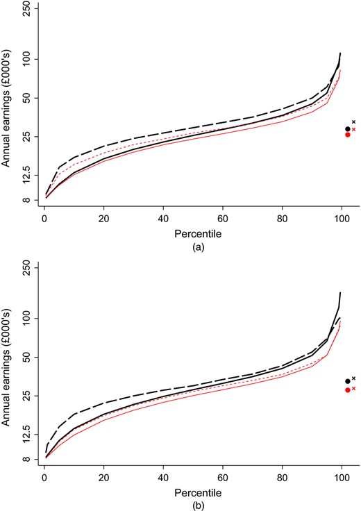
Graduate earnings, 1998–2003 cohorts pooled (non-parametric estimates of the LFS graduate and GS earnings distributions, for earnings greater than £ 8000; the left hand y-axis shows annual earnings on a log-scale and the right-hand axis shows the absolute percentage difference between the LFS and GS; conditional means are provided to the right of each picture (horizontal jitter is included to improve clarity); LFS earnings are weighted by using population weights) ( , males, GS;
  , mean;
  , females, GS;
  , mean;
  , males, LFS;
  , mean;
  , females, LFS;
  , mean): (a) 2008–2009 data; (b) 2011–2012 data
Returning to the full earnings distribution in Fig. 2, we observe considerably higher earnings in the LFS than in the GS in the lower parts of the distribution. The precise numbers are given in the on-line appendix C. In 2008–2009, at the 10th percentile, earnings are almost three times higher for men in the LFS (£ 15900) than in the GS (£5600) and twice as high for women (£ 12100 and £5900) respectively. The gap declines in percentage terms at higher levels of earnings but persists through the distribution up to the top tail. This is true for both genders in each of the five years that we investigate, with earnings only ever higher in the GS at or above the 99th percentile of the distribution. Consequently mean earnings (conditionally on working) are always higher in the LFS—by around 20% for men and slightly less for women. Indeed there is little difference in earnings between male and female graduates in their mid–late 20s and early 30s in the GS, whereas the differences in the LFS are larger.

The discrepancies between the GS and the LFS are striking and we consider a few potential explanations. First, lower earners may be less likely to respond in the LFS. Lower income individuals are more likely to be doing shift work, to have varied hours and to be more geographically mobile, which may make it more difficult to reach them longitudinally to complete the survey. Further, the low paid may be less inclined to complete the survey. For this to be the driving source of differences, this response issue must be gendered, with low earning men considerably less likely to respond than low earning women.
Second, LFS-reported earnings are subject to measurement error, caused by annualizing earnings from sometimes shorter periods. Around 60% report earnings for periods of less than a year, and those individuals typically have lower earnings than those who report earnings over a 1-year period. Individuals with very low earnings are likely to spend periods of the year out of work and this is ignored in such calculations. This explanation is supported by the fact that the discrepancy between the GS and the LFS is larger in 2008–2009 than in 2011–2012, which was a time when the labour market was more turbulent, but it would be more convincing if the share of those on zero earnings were greater in the LFS than in the administrative data, which is not so. A more convincing explanation is that the LFS excludes the earnings of individuals with variable pay. Our analysis here essentially assumes that the data are randomly missing earnings information from the set of individuals in employment. In practice this is unlikely, and this is instead likely to underestimate the share of individuals with low earnings.
Third, the LFS excludes self-employed earnings. Referring to Table 4 we see that around 45% of the fully self-employed earn below £8000. However, since this accounts only for less than 4% of individuals, excluding these individuals from the tax data would reduce the share earning between £0 and £8000 by only around 1.5 percentage points, which is a small fraction of the overall difference.
Fourth, employee pension contributions are excluded from the GS. This could plausibly explain a large share of the differences in earnings between the data sets above the median. According to the Office for National Statistic figures, average employee contributions are 6% of earned income and, although our own calculations from the British Household Panel Survey suggest that these are much smaller for 20–30-year-olds, they increase considerably with earnings—we estimate that they explain around half of the differences above the median for men and more for women. However, this is highly unlikely to explain the differences at the bottom of the distribution.
A final explanation is that the differences are instead driven by under-reporting of earnings in the GS. There may be earnings that people simply do not report to the tax office, such as earnings for cash-in-hand overtime work, to avoid paying tax or to receive in-work benefits. This is likely to be important when looking at the low paid. This would result in the proportion of individuals reporting very low earnings being higher in the official data than in the LFS, with the latter collecting a more realistic assessment of total earned income. However, this issue may also be relevant when considering gender differences; from the unconditional figures, it is clear that the LFS shows a stronger gender gap than does the GS. Potentially this would imply that males are more likely to have second jobs and additional sources of income that they include in their reporting to the LFS but that they do not declare to the tax office. Our conclusions for the LFS are unchanged by excluding earnings from second jobs but it is possible that individuals provide aggregate estimates of their earnings from all jobs when responding to the income questions in the LFS and hence this could still be an explanation.
In summary, there are various potential reasons why earnings are lower in the GS than in the LFS and we have no definitive explanation, particularly for the share of low earners. It is, however, important from a policy perspective to observe that the official tax record is the relevant record in terms of both tax contributions and repayment of student loans.
5.2. Labour Force Survey non-graduate and administrative data non-higher-education comparison
We now turn our attention to non-graduates. In the LFS these individuals are those who have not achieved a higher degree or equivalent, whereas for the administrative data we use the corrected SS, as described in Section 3.2.1. Table 9 compares the share of individuals who were not employed and, conditionally on working, the share reporting earnings between £0 and £8000. As for graduates, although the overall share of those not in employment is very similar across the two surveys, there are considerable gender differences in the LFS which do not exist in the administrative data. As previously described, we were particularly concerned about the share of low earnings in the SS due to issues with the ‘never-filers’, i.e. those who never file a return with HMRC, and with immigration. For these factors to be driving the results, never-filers would have to be predominantly women, whereas immigrants would have to be predominantly men. Although this is plausible, these patterns are similar for the GS where these issues do not apply.
LFS and corrected SS: non-graduates not employed and with low earnings overall and by gender for 2008–2009 to 2012–2013†
| Years | Results for % not employed | Results for % earnings < £ 8000 given earnings> £0 | ||||||||||
|---|---|---|---|---|---|---|---|---|---|---|---|---|
| Sample size | Share | Sample size | Share | |||||||||
| All | Males | Females | All | Males | Females | All | Males | Females | All | Males | Females | |
| LFS | ||||||||||||
| 2008–2009 | 16326 | 7759 | 8567 | 27.0 | 17.2 | 37.3 | 2942 | 1484 | 1458 | 11.7 | 4.2 | 20.9 |
| 2009–2010 | 14920 | 7021 | 7899 | 30.1 | 21.0 | 40.0 | 2594 | 1326 | 1268 | 13.2 | 4.8 | 24.5 |
| 2010–2011 | 14382 | 6925 | 7457 | 28.2 | 17.5 | 40.1 | 2430 | 1261 | 1169 | 13.0 | 4.1 | 25.5 |
| 2011–2012 | 14041 | 6828 | 7213 | 28.3 | 18.1 | 39.8 | 2481 | 1278 | 1203 | 13.9 | 4.3 | 28.8 |
| 2012–2013 | 10495 | 5082 | 5413 | 27.6 | 16.3 | 40.1 | 1778 | 946 | 832 | 15.4 | 5.4 | 29.9 |
| HMRC non-HE | ||||||||||||
| 2008–2009 | 243099 | 132522 | 110577 | 29.1 | 28.5 | 30.0 | 172245 | 94816 | 77429 | 37.4 | 33.7 | 42.0 |
| 2009–2010 | 243099 | 132522 | 110577 | 31.4 | 30.1 | 32.9 | 166805 | 92588 | 74217 | 37.6 | 34.5 | 41.5 |
| 2010–2011 | 243099 | 132522 | 110577 | 29.9 | 28.8 | 31.2 | 170451 | 94392 | 76059 | 38.0 | 34.7 | 42.0 |
| 2011–2012 | 243099 | 132522 | 110577 | 29.0 | 27.7 | 30.6 | 172581 | 95870 | 76711 | 38.9 | 34.7 | 44.3 |
| 2012–2013 | 243099 | 132522 | 110577 | 28.8 | 27.6 | 30.2 | 173102 | 95966 | 77136 | 38.7 | 33.9 | 44.7 |
The 1998–2003 cohort are pooled for each year. Note that the share not employed in the corrected SS is equal to the share not employed in the SS as the econometric correction corrects only the positive earnings distribution.
Fig. 3 shows the distribution of earnings for those with earnings above £ 8000 and for the entire distribution combined. Above £8000, the distributions are quite similar, with the LFS reporting higher earnings at the lower end of the distribution and lower earnings at the higher end. For the full distribution, we have a similar story to that for the graduate comparison, with the LFS reporting considerably higher earnings at the low end of the distribution. There is again more gender disparity in the survey data than in the tax data, although there is clearly a much greater gender difference in the non-HE sample than in the GS.
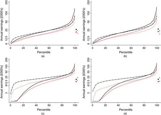
Similar to Figs 1 and 2, non-graduate earnings, 1999 cohort (precise numbers are given in the on-line appendix) ( , males, corrected SS;
  , mean;
  , females, corrected SS;
  , mean;
  , males, LFS;
  , mean;
  , females, LFS;
  , mean): (a) 2008–2009 data, earnings greater than £ 8000; (b) 2011–2012 data, earnings greater than £ 8000; (c) 2008–2009 data, all earnings; (d) 2011–2012 data, all earnings
Some of the potential explanations that were rehearsed in respect of differences between the GS and the LFS for graduates’ earnings also apply to non-graduates’ earnings. In addition to this, the immigration issue also affects the positive earnings distribution if overseas workers work for a fraction of the year and then leave the country. However, this is unlikely to be the whole story, and the very similar pattern for graduates suggests that similar factors might be at work.
5.3. Graduate and non-graduate combined comparison
Finally, we compare the results from the LFS with those from the combined GS and SS in Fig. 4. We use the SS rather than the corrected SS distribution as we are looking at the whole distribution together, so it does not matter if some graduates are misclassified as being in the SS. Conditionally on earnings being above £8000, the LFS and the combined administrative data earnings distributions are somewhat more similar. When considering the full distribution, unsurprisingly the familiar patterns again emerge, with a much higher share of low earners and much less gender disparity in the administrative data.
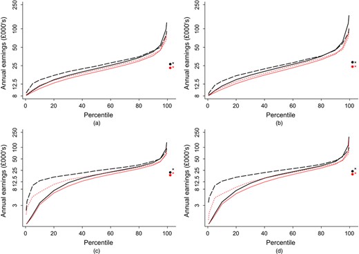
Similar to Fig. 1 combined with Fig. 2, graduates and non-graduates combined, 1999 cohort (precise numbers are given in the on-line appendix) ( , males, GS and SS;
  , mean;
  , females, GS and SS;
  , mean;
  , males, LFS;
  , mean;
  , females, LFS;
  , mean): (a) 2008–2009 data, earnings greater than £ 8000; (b) 2011–2012 data, earnings greater than £ 8000; (c) 2008–2009 data, all earnings; (d) 2011–2012, all earnings
Given these discrepancies, we have also (with help from colleagues at the Institute for Fiscal Studies) undertaken a comparison of the share earning below £8000, conditionally on working, by using the Family Resources Survey, which is another commonly used source of data with information on workers’ earnings. The Family Resources Survey suggests that around 17% of men and 27% of women in their late 20s were earning between £ 0 and £ 8000 in 2011–2012 (in 2012 prices). These numbers are both higher than in the LFS: considerably so for men. The females share is very close to the administrative data figure for women but still considerably lower for men. Our reasoning above would suggest that under-reporting of earnings is likely to be a significant cause of this but again we stress that the official tax record is the relevant source of data for many important policy purposes, including repayment of student loans.
6. Applied comparisons
Thus far we have shown comparisons of the cross-sectional distributions of the administrative and survey data. In this section we turn our attention to the implications of these findings for measuring the gender wage gap, the graduate premium and earnings inequality. In our on-line appendix E we also show graduate and non-graduate earnings growth in the 5 years following the recession. Each of these measures is of crucial importance for policy.
6.1. The gender wage gap
The gender wage gap is of considerable policy interest as large differences in pay by gender are known to have existed for a long time. We explore this in Fig. 5, which shows the gap at various points in the positive earnings distribution, for the LFS and administrative data. We do this for both graduates and for non-graduates, showing ratios through the distribution for 2008–2009 and 2011–2012 for the 1998–2003 cohorts combined. Ratios for 2009–2010, 2010–2011 and 2012–2013 are shown in the on-line appendix F.
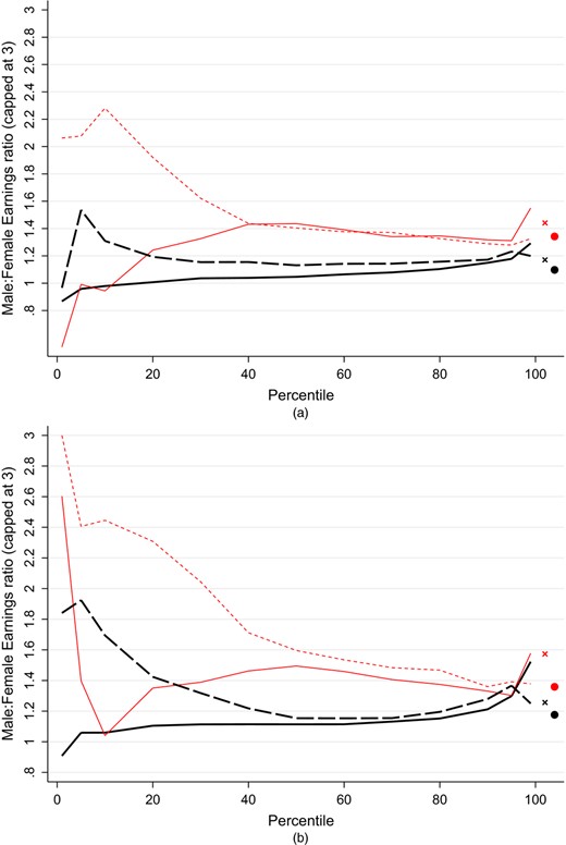
Ratio of male versus female earnings at different points in the distribution in the administrative data and in the LFS in 2008–2009 and 2011–2012 for the 1998–2003 cohorts combined, by graduate status (see the on-line appendix for raw numbers behind these figures and for other years) ( , administrative, graduates;
  , mean;
  , administrative, non-HE;
  , mean;
  , LFS, graduates;
  , mean;
  , LFS, non-graduates;
  , mean): (a) 2008–2009 earnings; (b) 2011–2012 earnings
We find that the pay gap between men and women is larger for non-graduates than for graduates, suggesting that HE plays a role in alleviating gender differences in earnings. This result is more pronounced in 2011–2012 than in 2008–2009, which could be driven by age effects. Above the 40th percentile, we find that the LFS and administrative data ratios are actually very similar, at around 1.1–1.2 for graduates and 1.4–1.5 for non-graduates. At the bottom of the distribution, however, the sources of data give very different results, with much less gender difference in the administrative data. These differences have further impacts on the mean male:female earnings ratio, with the survey data suggesting a greater wage gap than do the administrative data.
6.2. Graduate versus non-graduate earnings
The ratio of graduate to non-graduate earnings is important for those considering the value of studying for a degree (we refer to this as the graduate premium, though the differences here are descriptive rather than causal). In Fig. 6 we show the ratio of graduate to non-graduate earnings at various points in the positive earnings distribution for 2008–2009 and 2011–2012 (other years are provided in the on-line appendix F), for the 1998–2003 cohorts combined.
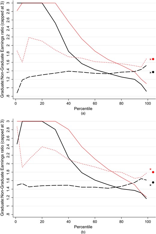
Ratio of graduate versus non-gradaute earnings at different points in the distribution in the administrative data and in the LFS in 2008–2009 and 2011–2012 for the 1998–2003 cohorts combined, by gender (see the on-line appendix for raw numbers behind these figures and for other years; the ratio is capped at 3) ( , administrative, males;
  , mean;
  , administrative, females;
  , mean;
  , LFS, males;
  , mean;
  , LFS, females;
  , mean): (a) 2008–2009 earnings; (b) 2011–2012 earnings
The graduate earnings premium is larger in the administrative data than in the LFS at the lower percentiles of the earnings distribution, though the premia in the two data sets converge further up the distribution. On average across the two data sets the graduate wage premium is around 1.7 and 1.4 for women and men respectively in 2008–2009 and 1.8 and 1.5 respectively in 2011–2012. Hence the graduate premium is larger for both women and men in 2011–2012 than in 2008–2009, suggesting more growth in graduate earnings for individuals in their late 20s and early 30s. At the very highest percentiles, the administrative data show lower graduate:non-graduate ratios. This may partially reflect the inadequacies of the non-HE sample, which is the result of an econometric correction to the SS to allow for the fact that the SS includes graduates who do not borrow. It is possible that the correction that we use is particularly weak at the higher end of the distribution due to the increased likelihood of the presence of graduates in that part of the distribution.
6.3. Earnings inequality
Finally, we consider earnings inequality in our various data sources. In each case, we sort n earnings as Y[1],Y[2],…,Y[n]. The Lorenz (1905) curve plots Ln(s), the cumulative share of earnings, against the population fraction s ∈ [0, 1]:
where ⌊x⌋ generically denotes the integer part of x. The Gini coefficient summarizes the curve as twice the area between the 45∘ line and the curve (alternative measures include the Atkinson (1970) index). In Table 10 we report Gini coefficients for 2008–2009 to 2012–2013, for each year pooling across the 1998–2003 cohorts.
Gini coefficients for the administrative data and LFS positive earnings distributions, split by gender and graduate status for 2008–2009 to 2012–2013†
| Year | Results for graduates | Results for non-graduates | ||||||
|---|---|---|---|---|---|---|---|---|
| Men | Women | Men | Women | |||||
| GS | LFS | GS | LFS | Corrected SS | LFS | Corrected SS | LFS | |
| 2008–2009 | 0.360 | 0.259 | 0.332 | 0.263 | 0.505 | 0.246 | 0.509 | 0.304 |
| 2009–2010 | 0.372 | 0.252 | 0.337 | 0.268 | 0.510 | 0.240 | 0.515 | 0.319 |
| 2010–2011 | 0.380 | 0.268 | 0.347 | 0.272 | 0.525 | 0.255 | 0.520 | 0.355 |
| 2011–2012 | 0.388 | 0.262 | 0.358 | 0.283 | 0.523 | 0.255 | 0.540 | 0.340 |
| 2012–2013 | 0.395 | 0.283 | 0.375 | 0.287 | 0.528 | 0.251 | 0.540 | 0.370 |
Table 10 shows that inequality generally rises between 2008–2009 and 2012–2013, probably because of a combination of the financial crisis and age effects as we hold cohorts fixed. There is considerably less earnings inequality in the LFS than in the administrative data, which is unsurprising given the dramatically higher earnings in the LFS at the bottom of the distribution. Earnings inequality is much greater for non-graduates than for graduates in the administrative data. This pattern is less clear for males in the LFS.
7. Conclusion
This paper compares earnings distributions from administrative tax records with LFS survey data. Understanding the strengths and weaknesses of these types of data sets and their use in the study of graduates’ earnings is important as the use of administrative data by policy makers becomes more prevalent in the UK and world wide. Broadly we find that the administrative data show lower mean earnings for both graduates and non-graduates and in particular suggest a far greater proportion of individuals with earnings below £ 8000 than does the LFS.
We explored various possible reasons for this difference in the distributions, including under-reporting of earnings in the administrative data and response bias and measurement error in the survey data. Although the LFS is likely to suffer from biases, the administrative data also suffer from biases that particularly affect the lower parts of the distribution. In addition, there are some specific issues when using the administrative data to analyse the earnings of graduates. Specifically, the GS records the earnings of individuals who study in England but then move abroad as 0 includes individuals who drop out of their degree without graduating and does not include graduates who did not borrow. All three of these factors could also bias downwards estimates of graduate earnings. However, the fact that we obtain a very similar pattern of differences when comparing the LFS with the administrative data for non-graduates suggests that the unique selection issues of the GS are not the main drivers of the differences at the bottom end of the earnings distribution. More likely explanations include sample selection resulting in low response in the LFS from low earners—in particular the exclusion of those with variable pay—that is not sufficiently captured in the population weights, systematic overreporting of earnings in the LFS by low earners or significant under-reporting of income from employment by lower earners in the administrative data. There is some evidence for the former problems, as estimates of graduates’ earnings by using the Family Resources Survey are far more closely aligned with the administrative data, particularly for females, though there is still a higher proportion of males in the administrative data with very low earnings. The under-reporting issue in the administrative data could perhaps be due to people doing casual unreported work or due to shifting their earnings into other forms of income, to avoid paying tax or to qualify for working tax credits. The greater share of self-employed people with no or low earnings seems to support this.
These differences between the two data sets have several important implications for our empirical findings. The LFS data suggest less earnings inequality, particularly for non-graduate men and a considerably larger gender gap. We also find that the LFS data paint a less favourable picture of the economic advantage of HE, as it exhibits a smaller graduate: non-graduate earnings ratio. We also show in the on-line appendix E that the administrative data display a smaller negative earnings shock for graduates in the years following the Great Recession—in both data sets, the decline in real earnings after the recession is large for graduates but the decline for non-graduates is larger in the administrative data. Hence, overall, the differences between the data sets are substantively important for policy research.
In summary, the new administrative data set has great potential for research, and may result in different conclusions about important labour market issues. However, we also raise issues about the reliability of the administrative data at the lower end of the earnings distribution which merit further debate and study. Overall we might think that the administrative data are likely to be more reliable than survey data at the upper end of the distribution because of their more comprehensive coverage and the legal obligation for accurate reporting. Further, it is of course the official earnings record on which calculations of tax take and graduate loan repayments are based, and therefore of great practical importance. Improving our understanding about whether the official earnings data are significantly under-reporting the earnings of individuals at the lower end of the earnings distribution is also a pressing issue, not just to ensure that we have accurate information on individuals’ earnings for tax purposes but also because of the current policy importance of earnings inequality and its apparent sensitivity to the source of data being used to measure it.
Discussion on the paper by Britton, Shephard and Vignoles
Jo Swaffield (University of York)
This paper provides a valuable and timely contribution on the usefulness of administrative tax records in assessing the earnings premium for graduates, and the income contingent returns on UK student loans. The paper contains an extremely careful and thorough approach to using UK administrative tax records that have been explicitly linked with the Student Loan Company (SLC) records via the national insurance number (which is unique to each individual worker). Britton, Shephard and Vignoles provide a very detailed analysis of two samples: one defined as the ‘golden sample’ (GS) where individuals are identified in the linked sample of SLC ‘administrative tax records’ as those taking out an SLC loan, and those in the ‘silver sample’ (SS) who do not.
One of the clear strengths of the paper is that the sample of administrative tax data worked with is the actual record used to inform (and indeed to collect) the graduates’ repayments on their student loans. Further, the samples comprise long panels of data with additional links to higher education providers and subject choice allowing breakdowns by subpopulations (though this was not exploited in this paper). The authors have constructed an important data resource that can be usefully compared with other well-established large-scale labour market surveys. Comparisons with the Labour Force Survey will be useful to both academic researchers and government departments on a range of key policy issues, e.g. the returns to higher education, gender pay gaps, earnings inequality and, critically, the numbers of graduates earning at such low levels (conditionally on working) that they are unlikely to pay back income contingent student loans.
Of course, with all samples and data there are limitations, so some comment must be made on how convincing these two constructed samples, the GS and SS, actually are. The GS defines ‘graduates’ as those taking out a loan rather than necessarily completing a degree programme, and the SS defines the counterfactual group of ‘no degree’ through the absence of an SLC loan. This classification is not perfect, and the SS is likely to become less convincing in the future as we move towards higher skilled migration to the UK (as non-UK graduates are classified into the SS) and as the uptake of UK degree level apprenticeships increases. Further, the most informative comparisons of these administrative data with other labour market surveys will require using the Annual Survey of Hours and Earnings alongside the Labour Force Survey, thereby allowing a triangulation of data findings, particularly around issues such as the gender pay gap.
In highlighting both the strengths and the weaknesses of the administrative data the authors clearly show the value—through creativity and rigour—that academic researchers can bring when working with (existing) government administrative data resources. So, on that point, a note must be made on the ‘environment’ within which this key research project has been undertaken. There is likely to be little that strikes greater fear into the heart of an academic researcher than the statement on the sixth page that
‘… our work was carried out in a highly secure data enclave within an HMRC facility. … checked by officials …’.
Although research using (government) data should always be carried out professionally, respectfully and with appropriate consideration of ethical implications, it can seem at times that the barriers to ensure this data protection have become so arduous that academics are being discouraged from working with key data sets that are critical to inform the evidence base on key policy questions so needed by government.
Finally, using large-scale administrative tax records to understand the outcomes or returns from education is informative. It is certainly true that earnings (as reported in the tax record) provide a key outcome of education; however, they are far from the only variable of interest, and especially so for economists. For example, earnings are just one dimension of ‘employment’ that is positively affected by an individual's level of education. More generally higher education can be viewed as transformative for an individual's life course, and through positive externalities is also transformative for our wider society and economy. The contribution of UK universities to this is key and should be viewed in a context wider than just as an education provider. Universities embody a broader societal contribution as engines for economic growth and innovation, and as hubs for the creation and dissemination of knowledge. Universities are key anchor institutions within our cities and regions, creating wider economic activity, opportunities and positive outcomes for a range of citizens far beyond the student communities that we also serve. Such a broader context for considering the contribution of UK universities is particularly relevant now as we await the ‘Review of post-18 education and funding’ which is due in the spring of 2019.
Roger Smith (Cardiff)
I extend my thanks to the authors for this paper. We view the future of many statistics as being based on administrative data, and research of this type is critical to help to develop solutions.
About the analysis
I found the paper accurate in considering the specifics of Labour Force Survey (LFS) data collection. However, there are a few things I should like to pick up on.
Firstly, more focus could be paid to the LFS asking earnings to only people who conducted paid work in a reference week. Her Majesty's Revenue and Customs (HMRC) recognized, in its Pay As You Earn ‘real time information’ (PAYE RTI) experimental statistics publication Her Majesty's Revenue and Customs (2009) that this is likely to suppress the number of people working and earning in the LFS compared with administrative data which might have a broader coverage (their RTI analysis is based on pay received during a tax quarter). HMRC's analysis indicated that this produces an RTI estimate of people in work that is approximately 7% higher than for the LFS.
The Office for National Statistics, meanwhile, has compared LFS responders with PAYE data and found a slightly higher response rate among households who have a positive income on PAYE (see Table 2 from Office for National Statistics (2017)).
The two points together raise the question of why we do not obtain a bigger difference between the percentage of people reported as having zero income in the two sources in this paper.
Secondly, the report suggests that the LFS might have a lower response among low earners. For example, it might miss shift workers, or those who are more mobile. But actually the LFS is probably good at picking up these kinds of people because the sample is based on addresses rather than individuals. Also, interviewer calls are spread throughout the day and evening, meaning that shift workers should not be missed.
We might envisage slightly lower response rates at the low end of the earnings scale, but we would expect to see a similar pattern among highest earners. That does not come through in the paper, and we feel that it should looked into as a priority.
Thirdly, a notable finding in the paper is the difference between men's and women's pay.
The paper presents the proportion of graduate women earning less than £8000 a year in the LFS as about double that for men. Among non-graduates the differential is about five or six times. If graduates account for approximately 50% of those aged 22–29 years, that would put the differential as approximately four times as many women earning under £8000 a year.
The administrative data have a differential of less than 1.5:1.
To help to give a perspective, the Office for National Statistics promote the Annual Survey of Hours and Earnings (ASHE), which is the main source of gender pay gap estimates. I view the ASHE as very relevant especially because it collects its information from employers rather than workers.
The ASHE publishes data tables based on age bands, most relevant being weekly gross earnings among 22–29-year-olds (for 2009).
To have an annual salary of £8000, people would have to earn roughly £160 a week if working constantly, and more if not. The figures in Table 11 show that the 10th percentile for men (£ 205) and the 20th percentile for women (£ 196) are sufficiently close to this figure to project that the differential between men and women earning less than £ 8000 a year might be approximately 2:1.
Gross weekly earnings among 22–29-year-olds by sex†
| Percentile | ASHE 2009 weekly pay (£) | |
|---|---|---|
| Males, 22–29 years old | Females, 22–29 years old | |
| 10th | 204.8 | 118.3 |
| 20th | 269.8 | 196.1 |
| 30th | 312.0 | 251.7 |
| Percentile | ASHE 2009 weekly pay (£) | |
|---|---|---|
| Males, 22–29 years old | Females, 22–29 years old | |
| 10th | 204.8 | 118.3 |
| 20th | 269.8 | 196.1 |
| 30th | 312.0 | 251.7 |
Source: 2009 ASHE.
That is in between the differentials from the two sources, suggesting that more exploration of both sources estimates is necessary.
Fourthly, with regard to graduates, the LFS figures in the paper (Table 8) suggest that approximately 6% in this age range in work earn below £8000, whereas the gold sample estimates approximately 14%.
For non-graduates (Table 9) the LFS suggests that 15% of this in this age range in work earn below £8000, and in the silver sample it is 38%.
If we assume a 50:50 split between graduates and non-graduates, overall the LFS will calculate roughly 10%, and the administrative data to approximately 26% earning less than £8000.
The profile from the ASHE, meanwhile, suggests a proportion that is much closer to 10% (Table 12).
Gross weekly earnings among 22–29-year-olds†
| Percentile | ASHE 2009 weekly pay (£), all 22–29 years old |
|---|---|
| 10th | 146.6 |
| 20th | 235.2 |
| 30th | 283.9 |
| Percentile | ASHE 2009 weekly pay (£), all 22–29 years old |
|---|---|
| 10th | 146.6 |
| 20th | 235.2 |
| 30th | 283.9 |
Source: 2009 ASHE.
Note that both the LFS and the ASHE collect earnings information for only employed people or jobs. The self-employed are a low proportion of workers, but they may be heavily skewed to reporting lower earnings to explain the difference between the two sources.
Summary
The authors could not link individuals between the two sources of data. Profiling the cases with the biggest difference between the two sources would give a much clearer indication of the causes. The LFS has a large base of variables to work from, and I look forward to increased use of wider data for these purposes.
The vote of thanks was passed by acclamation.
Tom King (Newcastle-upon-Tyne)
Ethical oversight of research using emerging data is nascent, specifically here reliance on the idea of a ‘social licence’ in place of subject consent. Research accessing vast amounts of administrative records makes individual consent infeasible—public benefit is required for access to be approved, but this decision is made by a data access committee, on the behalf of subjects, so subjects are neither consenting nor informed. The outcome of the analysis is not harmful, but the sensitive personal data usage, and particularly its linkage, has never been notified to subjects. Income data is a sensitive item in surveys in the UK, so the use of these data acquired administratively should not be automatic.
Access procedures for such data take time, a point which Britton, Shephard and Vignoles note, with more tone of entitlement than seems justified by the ethical process followed. Ethical review is broken into pieces in a project of this kind, with institutions, funders and data owners all involved (UK Research Integrity Office, 2017) without yielding a coherent assurance. Historically, data collection and the artificial treatment of subjects for research purposes have been regulated, to prevent harms; ethical analysis has been taken for granted, regulated by the professional ethics of the analyst, yet professional codes need updating for new data (Organisation for Economic Co-operation and Development, 2016).
Formal concern about data ethics is all very recent, as shown in Table 13, and certainly since the research reported in the paper was reviewed. For example, in 2013, the Organisation for Economic Co-operation and Development had not turned its attention to emerging data, focusing on ‘new’ types from the Internet of Things, sensors, social media etc. (Organisation for Economic Co-operation and Development, 2016). Since the collapse of care.data in 2014, which brought home the complacency of a social licence to use routine data for other purposes (Carter et al., 2013), new ideas have emerged. Some kind of subject consent should be sought, using a detailed consultation method such as citizen juries, or by engaging a community group with appropriate authority (Organisation for Economic Co-operation and Development, 2016): and coherent interdisciplinary consideration of the proposed research, so that both technicalities and sensitivities are integrated (Murtagh et al., 1982). The nature of social licence, such as respecting the dignity of groups (in this case young graduate debtors), in national guidance has moved on accordingly. What to do if social licence changes during the course of a project is something statisticians will need to resolve—others do not do sufficiently complex projects.
Chronology of concepts for ethics in secondary data during research
| Year | Publisher | Title | New concept |
|---|---|---|---|
| 2012 | Department of Homeland Security | Menlo report | Public interest |
| 2013 | Organisation for Economic Co-operation and Development | New data for understanding the human condition | New data |
| 2015 | Insight | A Magna Carta for data | Data rights |
| 2016 | Royal Statistical Society | The opportunities and ethics of big data | Data ethics council |
| 2016 | National Data Guardian | Review of data security, consent and opt-outs | Direct care |
| 2016 | Organisation for Economic Co-operation and Development | Ethics of economic and social research | Emerging data |
| 2016 | National Statistician's Data Ethics Advisory Committee | Revised terms of reference | Ethics not access |
| 2016 | UK Research Integrity Office | Internet mediated research | Institutional codes |
| 2017 | British Academy and Royal Society | Data governance and data management | Data stewardship |
| 2018 | Expert Advisory Group of the European Data Protection Supervisor | Report of expert group | Dignity of groups |
| 2018 | Managing Ethico-social, Technical and Administrative Issues in Data Access | Better governance, better access | Interdisciplinarity |
Job de Roij and Catherine Bromley (Office for Statistics Regulation, Edinburgh)
Statistics add value when they answer society's questions. But, many of those questions cannot be answered without sharing and linking data. A greater willingness and ability to share and link data is therefore essential for improving statistics. Our review of data linkage in the UK statistics system (Office for Statistics Regulation, 2005) identified a gap between what is possible in terms of valuable insights from data linkage and what is currently achieved. Value is being squandered because data linkage is too difficult and too rare. The study of Britton, Shephard and Vignoles is an excellent example of how greater access to different sources of data creates new opportunities to answer society's questions.
The authors combined administrative data from three sources (Her Majesty's Revenue and Customs tax records, Her Majesty's Revenue and Customs self-assessment databases and Student Loan Company records) to provide insights about individuals’ earnings. They harness the power of large-scale administrative data to address questions about the gender wage gap, the graduate premium and earnings inequality. These insights were only possible by linking these different data sources; no single source could have achieved this.
Importantly, the study investigates the strengths and weaknesses of the linked data set. Much of what we know about individuals’ earnings comes from government sample surveys, which have well-known limitations. For this reason, researchers are increasingly looking to administrative data to understand what is happening with earnings. But, as the authors demonstrate, administrative data sets also have weaknesses, such as potential under-reporting of earnings in particular income groups. Without this focus on, and understanding of, data quality, results can be misleading. Survey and linked administrative data may provide different answers to the same questions, and it is important to understand why. Our review includes recommendations to improve the quality assurance of linked data.
Academics and independent researchers provide vital additional input as analysts outside government. In this regard, we welcome the Digital Economy Act's research provisions, which will support external users with an interest in accessing government data. Enabling access to data for research purposes adds value to the statistics system—by identifying important questions to be answered, conducting analyses that government does not have the capacity to do and opening up data to scrutiny via secondary analysis. This study clearly showcases these benefits of linked data, and we look forward to such studies becoming the norm rather than the exception.
Paul A. Smith (University of Southampton)
I welcome the general approach to the use of linked administrative data under appropriate access conditions. In this response I shall focus on the quality of the data sources compared, rather than the substantive results. This paper presents an interesting example where the data quality from both the linked administrative and the corresponding survey sources are subject to errors. In this case the data are linked deterministically through national insurance numbers and, although there may be some minor issues related to temporary national insurance numbers, the linkage is likely to be effective. However, since the analysis depends on the linkage, some follow-up of cases which did not link might have been useful, to understand whether they were errors, or just cases that should not link.
It is well recognized that administrative data are not collected directly for statistical purposes, and therefore that some definitions are not ideal for the analyses we would like to do. However, there has been less investigation of measurement errors and ‘respondent’ interactions with administrative systems, so the errors in those systems are less well known statistically. However, survey data are also subject to biases and other errors, and in this particular example the response rates in the Labour Force Survey (LFS) have been declining, which makes it potentially more susceptible to selection effects. However, the LFS questionnaire is specifically designed and targeted at high quality measurement of variables of interest.
This paper presents very interesting observations on the differences in the two approaches. It is not clear which is better, as there are errors on both sides. In a perfect world I would wish for ‘total error’ evaluation (like total survey error (Groves and Lyberg, 1970) but adapted where necessary for administrative data). Perhaps the eventual arbiter would be to match the LFS data with tax information (which has been done experimentally with Pay As You Earn; see Office for National Statistics (2017)). The LFS does not collect national insurance numbers, however, so in this case the match would not be deterministic and it would be important to account for linkage error in analyses (Smith and Chambers, 2001).
Paul Allin (Imperial College London)
Administrative data sets are increasingly used in research, though perhaps more slowly than expected. Thanks therefore go to Britton, Shephard and Vignoles for this welcome addition to the literature and for sharing their experience, hopefully pour encourager les autres.
Hand (1981) recently identified many challenges in using administrative data in statistical analysis. Clearly the authors had to tackle many of those. It would nevertheless have been useful to learn more about the strengths and weaknesses of the administrative and financial data used here, especially as the concept of earnings needs to cope with an evolving labour market, including portfolio careers and working in the ‘gig’ economy, with its proliferation of short temporary contracts between companies and independent workers.
Looking particularly at Student Loan Company data, how was the estimate of 85–90% coverage obtained, and what is known about characteristics of graduates who did not take up a loan? This is a reminder that, contrary to a widespread view of administrative data ‘n does not always equal all’.
Can the authors then say more about why they did not use the full set of Her Majesty's Revenue and Customs administrative data? They may have a ‘golden’ sample, but it is still a sample from the full set of records, which seems to run counter to the ambition of using big data sets.
Finally, I would like to comment on the utility of this analysis and specifically how far do the authors see it important to address that? It seems to me that their results are effectively official statistics because they draw fully on official data. (The Student Loan Company is a non-departmental public body established to administer a scheme, within the policy context and legislative framework laid down by the government). All official statistics should meet the test of practical utility. Yet I am left feeling that the authors have added to the supply side—resources for future researchers—without considering the demand side. How are their results to be communicated and used? Who are the policy audiences? What are the messages for those yet to start a course of further or higher education and to consider taking out a loan?
Further use of administrative data for research might just be encouraged if researchers are clear on the utility of the statistical analysis that they produce.
The authors replied later, in writing, as follows.
We thank the Royal Statistical Society for the opportunity to present our research and the various thoughtful discussants for their comments. These comments add much to our paper and we are most grateful.
The use of administrative data, particularly tax-type data, is potentially enlightening for many areas of economics and social science more generally. In particular, this kind of data is often exactly the correct data to look at for many issues in public economics, such as the study of student loan repayments, and does not suffer from problems of non-response which are a blight on other modern research methods.
However, these new data raise new issues for researchers, such as relating them to existing results and the data not being widely available which makes replication difficult, if not impossible. It also raises important and interesting questions over ethical behaviour as we use tax data and taxes are not, by definition, collected voluntarily. Instead the rules over tax collection and the use of data based on taxes are tightly prescribed by the public themselves through their representatives. In our case, the tax data rules are determined by detailed statutes written by the UK Parliament itself.
We are particularly grateful for the two respondents’ comments regarding the ethical use of data and specifically on the use of non-consented administrative data for research purposes. As far as our project goes, the proposal was reviewed from an ethical and legal perspective by several organizations including the two data controllers, namely the Student Loan Company and Her Majesty's Revenue and Customs (HMRC). The primary consideration with regard to the use of administrative data is that the project needs to be in the public interest. For HMRC, this requirement is very clear in that use of the data is permitted only when the analysis will be of benefit to HMRC in carrying out their duties, as is the case with this project. Naturally there are a range of other issues that also arise around the legal framework to permit linkage between two data sets (in this case the Student Loan Company data and HMRC data), ensuring confidentiality when results are reported and, of course, data security. In our case, the last two considerations were addressed by the work being done in a secure data laboratory, controlled by HMRC and from which all outputs were scrutinized by HMRC staff. More generally, as with any research project, the proposal was scrutinized under the Universities of Oxford and Cambridge ethics procedures. From our perspective, although individuals have not given explicit permission for the data on them to be used in this way, the public benefit arising from the analysis is significant and we were satisfied that this is an ethical and legal use of the data.
All that said, the respondents raise important issues about when it is appropriate to use administrative data for research, given that seeking consent from individuals in administrative data sets is likely to be infeasible, and indeed would have a major negative effect on the quality of the research given the likely low response rate. The potential for administrative data to provide important insights into a wide range of social and economic issues is huge. Linked administrative data can provide insights into topics as diverse as the socio-economic drivers of public health outcomes such as diabetes, the use and efficiency of public services and, as here, the economic value of investments that the state makes in education. Administrative data can also help us to understand the many inequalities that shape our society and can help us to generate the evidence that is needed to make inroads into reducing them. So the prize from linking administrative data is great indeed. There are, however, two challenges. The first is to ensure proper public debate on the use of data in this way, to make sure that we have a consensus on when and how it is appropriate to use routine administrative data for research that is in the public interest (as distinct from for commercial gain). Further, we need to convince the government of the value of linking administrative data to help it to do its business more effectively. The Administrative Data Research Partnership established by the Economic and Social Research Council in 2018 has been charged with doing just that. It will be vital that the Administrative Data Research Partnership not only secures the support of government departments to do the data linkage but also that it stimulates the public debate that is needed to reach broad consensus on when and when not such data can be used for research.
Our discussants raised three other main points: comparison with results from the Annual Survey of Hours and Earnings (ASHE), the gender pay gap and reminding us about the importance of the non-economic benefits of higher education.
Direct comparison with the ASHE is problematic given that the coverage of the two data sets is different. The ASHE is not an administrative source of data: rather it also is survey based. ASHE data are based on a 1% sample of employee jobs taken from HMRC Pay As You Earn records. Information on earnings and hours is obtained from employers. Further, the self-employed and those not paid in the week of the survey are not recorded in the ASHE. Hence, although the Labour Force Survey and the Family Expenditure Survey do appear to understate earnings relative to the ASHE, all three are survey methods with potential for non-response. Our argument is that the administrative data source that we have is less likely to suffer from this bias.
We are wholeheartedly in agreement that our paper does not measure the ‘gender pay gap’; what we measure is the gender difference between very well defined definitions of annual record earnings. The difference between our measure and the gender pay gap can come from many sources, such as different numbers of hours worked, different career choices and different wage rates. Our data set provides no way of breaking out our gender differences into these important categories. Other data sets will be far superior at understanding these drivers. However, the gender differences in annual earnings are important, as annual earnings drive many important aspects of the economy. They drive the tax take from women and men. They also drive how the government subsidizes men's and women's higher education differently. We think that quantifying these aspects and how they change through time is important, if not the only important question one could ask.
Finally, all three of us agree with Professor Swaffield in her appeal to look at the broader rewards that higher education provides to students. Our drive was to study how student funding in England works and how it might be improved, because we believe that large parts of higher education are good for the economy, and that higher education more generally allows the individual who is better educated to have a life with more choices. It is certainly a worthy goal to study the second aspect. We hope that the members of the Royal Statistical Society will think that it is also worthy to try to use statistics to improve how governments can use its limited resources to help to educate our fellow citizens.
Acknowledgements
This paper is a revised version of ‘Comparing sample survey measures of English earnings of graduates with administrative data during the Great Recession’. Here we exclude earnings dynamics. Many civil servants and policy makers have helped us to gain access to the data which are the core of this paper. We thank in particular Daniele Bega, Dave Cartwright, Nick Hillman, Tim Leunig and David Willetts for their invaluable contributions. We also thank A. B. Atkinson, Raj Chetty, Jonathan Cribb, Mark Gittoes, Chuka Ilochi and Jonathan Waller for their comments on previous drafts, and our advisory group, Alison Allden, Nick Barr, Danny Dorling, Josh Hillman, Robin Naylor, Kate Purcell and Ian Walker. We also thank our three referees for excellent comments. We solely are responsible for any errors. For financial support we are grateful to the Nuffield Foundation for original funding, and Jack Britton is also grateful to the British Academy. The views that are expressed are those of the authors and not necessarily those of the Foundation or the British Academy.
HMRC and the SLC have agreed that the figures and descriptions of results in the paper may be published. This does not imply HMRC's or SLC's acceptance of the validity of the methods used to obtain these figures, or of any analysis of the results. Copyright of the statistical results may not be assigned. This work contains statistical data from HMRC which are Crown copyright and statistical data from the SLC which are protected by copyright, the ownership of which is retained by the SLC. The research data sets that were used may not exactly reproduce HMRC or the SLC aggregates. The use of HMRC or SLC statistical data in this work does not imply the endorsement of either HMRC or SLC in relation to the interpretation or analysis of the information.
