


Summary
The paper considers the use of level-of-effort (LOE) paradata to model the non-response mechanism in surveys and to adjust for non-response bias, particularly bias that is missing not at random or non-ignorable. Our approach is based on an unconditional maximum likelihood estimation (call-back) model that adapts and extends the prior work to handle the complexities that are encountered for large-scale field surveys. A test of the ‘missingness at random’ assumption is also proposed that can be applied to essentially any survey when LOE data are available. The non-response adjustment and the test for missingness at random are then applied and evaluated for a large-scale field survey—the US National Survey on Drug Use and Health. Although evidence on non-ignorable non-response bias was found for this survey, the call-back model could not remove it. One likely explanation of this result is error in the LOE data. This possibility is explored and supported by a field investigation and simulation study informed by data obtained on LOE errors.
1 Introduction
It is well known in the survey methods literature that non-response to a survey is an important contributor of estimation bias (see Groves and Couper (1998) and Groves (2006)). Non-response bias can be substantial when response rates are low and the characteristics of respondents and non-respondents differ (Biemer and Lyberg, 2003). A common practice for reducing the bias is to adjust the survey weights so that the weighted estimates reflect both respondent and non-respondent characteristics. The weight adjustment essentially inflates a respondent’s selection weight by the inverse of the respondent’s response propensity or probability to respond to the survey (Little and Rubin, 2002). Analysis of the survey data can then proceed by using the adjusted weights to compensate at least partially for non-response in the analytical results.
Traditionally, the response propensities are estimated through a model, which is specified explicitly as a logistic regression model or implicitly through a non-response weighting class adjustment (Biemer and Christ, 2008). Most non-response models assume that non-response is ignorable or ‘missing at random’, i.e. the response mechanism does not depend on the missing data. Otherwise, the non-response mechanism is called non-ignorable and non-response is said to be ‘missing not at random’ (Rubin, 1976). As an example, non-response in surveys of drug use is often disproportionately higher among drug users than non-users, which can lead to negatively biased estimates of the prevalence of drug use. Because non-response is related to the outcome variable (drug use in this instance), it is non-ignorable. A weight adjustment that assumes ignorable non-response could still reduce the bias to some extent, but its effectiveness depends to a large extent on how well the missing data mechanism and the outcome variable are modelled in the adjustment process.
Traditional modelling approaches are restricted to using explanatory variables that are known for both respondents and non-respondents. These include frame variables, variables obtained through a screening interview and data collected during the interview process. The last type of data is often referred to as paradata in the survey methods literature (Couper and Lyberg, 2005). There has been much interest recently in developing modelling approaches that expand the pool of variables to include variables that may be known for respondents only, such as data collected during the interview. This admits the possibility of using any variable in the questionnaire in the non-response modelling process, thus compensating for non-ignorable non-response for these variables. One approach for incorporating ‘respondent-only’ data in the non-response adjustment and the topic of this paper is call-back modelling.
Call-back modelling incorporates information on the level of effort (LOE) that is applied to a sample member to obtain a final disposition (i.e. interview, refusal, other non-response or final non-contact). LOE data are known to be highly correlated with survey response rates (see, for example, Groves and Couper (1998), Groves and Kahn (1979) and Wang et al. (2005)). By modelling the response propensity as a function of the LOE, call-back models can incorporate respondent-only data. Then, through maximum likelihood estimation approaches, call-back models yield weight adjustments that can compensate for the non-response bias in the respondent-only variables. In this way, call-back models have the potential to compensate for non-ignorable non-response.
As described in some detail in the next section, the current approaches to call-back modelling have limited applicability because they require some assumptions that are not tenable in practice. The main objective of this paper is to propose a general modelling framework that addresses these limitations by relaxing some assumptions made by current approaches. Along the way, three additional objectives are addressed. After introducing the general modelling framework, the paper proposes a test of the missingness at random (MAR) assumption that can be performed after traditional non-response adjustments have been applied. Then the paper illustrates and evaluates the models proposed and test for MAR for a large-scale national survey of drug use—the National Survey on Drug Use and Health (NSDUH). Finally, considering the results of the NSDUH application, the paper uses simulation to demonstrate how call-back model adjustments can actually add bias to the estimates when LOE data are inaccurate, severely limiting the effectiveness of the non-response weight adjustment.
The approaches that are considered in this paper require access to LOE data which may only be available to data producers. However, as uses of paradata during data analysis expand (see, for example, Kreuter and Casas-Cordero (2010)), survey producers are beginning to release LOE and other paradata with the public use data files from the survey. This opens the possibility for data users to apply the approaches that are described in this paper in their analyses, possibly to refine the weights or to test the MAR assumption. Further, we note that, because weight construction is based on estimation of totals and means (see, for example, Biemer and Christ (2008)), the focus of the paper is on the population mean. However, the weights so obtained can be applied to any analysis where survey weights are required.
2 Background
The idea of using call-backs to adjust for non-response bias was first proposed more than 60 years ago. Politz and Simmons (1949) used an idea that was proposed by Hartley (1946) to develop a famous method of adjustment based on retrospective reports of availability. Although the Politz and Simmons adjustment is rather crude, it clearly demonstrates that a sample member’s contactability is related to many survey characteristics and can be an important factor in adjusting for non-response bias. As previously noted, it is now well known that response propensity is highly correlated with the number of call-backs that are made to a sample unit.
One approach for incorporating the number of call-backs in non-response adjustments is simply to include it as another variable in the traditional response propensity model and there are numerous examples of this in the literature (see, for example, Göksel et al. (1992), Groves and Couper (1998), page 314, and Kreuter et al. (2010)). Used as a model covariate, the number of call-backs often provides improved model fit, but its ability to compensate for the non-ignorable non-response is quite limited. Alternatively, likelihood approaches that use LOE data jointly with respondent-only variables can reduce the missingness not at random bias but, for the reasons discussed below, are seldom used in practical survey applications. Although various likelihood approaches for call-back modelling have been proposed in the literature, they can be ascribed to essentially two general frameworks: the full likelihood model that was proposed by Drew and Fuller (1980) and the conditional likelihood model that was proposed by Alho (1990).
Drew and Fuller’s (1980) model uses call-backs to estimate the population distribution of a categorical outcome variable G that is observed only for respondents in the sample. Their approach assumes that response propensities vary by the L categories of G and uses maximum likelihood estimation to estimate & pr ;(G = g), g = 1,…,L. They then used these estimates of & pr ;(G = g) to form a post-stratified estimator for any other survey variable, say X, thereby reducing the non-response bias in the estimate of , the population mean of X. To illustrate, let denote the respondent mean of X for G = g and let denote the call-back model estimate of & pr ;(G = g), g = 1,…,L. Drew and Fuller showed that
is unbiased for if response propensities are homogeneous within the categories of G, which is a typical assumption for weight adjustment approaches (Biemer and Christ, 2008). An interesting feature of Drew and Fuller’s model (see, also, Biemer and Link (2007)) is the option to include a latent indicator variable representing ‘hard-core non-respondents’, who are defined as non-respondents with zero probability of responding at every call-back.
An important limitation of Drew and Fuller’s approach is the assumption of a single action response process, i.e. that a call attempt either succeeds or fails in a single action. This assumption may be appropriate only for mail surveys where a request to participate results in either a returned questionnaire (response) or no return (non-response). In contrast, interviewer-assisted surveys involve at least two actions. First, an attempt is made to contact a sample member which results in either a contact or a non-contact. Then, if a contact is made, the interviewer attempts to complete an interview with the sample member. This action results in either an interview or a non-interview (refusal, inability to respond, language barrier, etc.). Biemer and Link (2007) extended Drew and Fuller’s approach to reflect these dual actions by specifying probabilities of contact and probabilities of an interview given contact. Further, they also showed how the EM algorithm can be used to obtain estimates of these probabilities and then used them to derive non-response weighting adjustments.
A very different approach was taken by Alho (1990). His modified conditional maximum likelihood approach also incorporates variables in the non-response adjustment process that are known only for respondents. However, Alho (1990) modelled the probability of a response at each attempt by a logit model and then substituted this model representation of the response propensities in a conditional likelihood of response given that a sample member ultimately responds to the survey. Wood et al. (2006) compared this modified conditional maximum likelihood approach with two other approaches:
- (a)
the full unconditional likelihood similar to Drew and Fuller (1980) but incorporating the EM algorithm (Dempster et al., 1977) for the estimation and
- (b)
the same model estimated in a Bayesian framework using the Gibbs sampler, a form of Markov chain Monte Carlo algorithm.
Interestingly, the choice of model does not seem to matter in their application. However, in a series of simulation studies, Kuk et al. (2001) found that the modified conditional maximum likelihood estimator, although consistent, can be biased and very inefficient (see also Wood et al. (2006)). Other similar approaches have been proposed by Anido and Valdés (2000), Potthoff et al. (1993) and Copas and Farewell (1998).
A criticism of most call-back models is that their simplifying assumptions seldom hold for practical applications. For example, except for Biemer and Link (2007), the models assume a single-action response process that has limited applicability for interviewer-assisted surveys, as noted above. Some models (e.g. Drew and Fuller (1980)) further assume that the probability of a response does not vary by call-back attempt which, as will be described later, is unrealistic in practice. The complex sample design is also often ignored, as are cases whose eligibility for the survey is unknown. And, except for Biemer and Link’s, the models do not take into account right-censored call-backs which occur when call attempts are prematurely terminated for some units. For example, right censoring occurs when, as proposed by Groves and Heeringa (2006), only a subsample of the non-respondents are pursued for an interview rather than all non-respondents (which is sometimes referred to as double sampling for non-response). Call-back censoring can also occur to adjust the sample size to some target number of respondents.
In addition, there has been no rigorous evaluation of the bias reduction capabilities of the approaches, relying instead on simulations, applications to artificial populations and model diagnostics to gauge the viability of the approaches. Biemer and Link (2007) provided one attempt to evaluate call-back modelling using real data while dealing with some of the problems that are associated with applications of call-back modelling to actual field work.
Extending Drew and Fuller’s approach, Biemer and Link (2007) applied a full likelihood call-back model approach to data from a random-digit dialling (RDD) telephone survey. Incorporated in their application were provisions to handle the complexities that are encountered in RDD surveys. For the present study, Biemer and Link’s approach will be further extended for application to a field survey, i.e. the 2006 NSDUH—an in-person, cross-sectional survey conducted in all 50 states and the District of Columbia designed to measure the prevalence and correlates of drug use in the US population aged 12 years or older. An important difference between centralized telephone and field data collections for call-back modelling is the quality of the LOE data. In telephone surveys, each call-back and its outcome are recorded automatically by the computer-assisted telephone interviewing system. In field surveys, interviewers must manually record each call-back and call outcome in the field management system. This manual process greatly increases the risk of errors in the LOE data. Yet, the robustness of the call-back model estimates to LOE data errors, which is evaluated in the present paper, has never before been examined.
In addition, for RDD surveys, call-back model adjustments may result in substantial reductions in non-response bias compared with the traditional adjustment approaches (Biemer and Link, 2007). Traditional approaches are often ineffective because so little information is available on non-respondents in RDD surveys (see Biemer and Link (2007)). Instead, the non-response adjustment is typically combined in a coverage adjustment using census totals that are highly aggregated (e.g. regional totals) and only weakly correlated with response propensity at an individual level. By contrast, field surveys often have extensive information for sample members from the frame, interviewer observations or, as in the present application, a screening interview with a high response rate. In general, traditional non-response adjustments are usually more effective for field surveys and, thus, incorporating LOE data in the adjustment process may be less beneficial than it was in Biemer and Link’s application. The current paper considers various issues in the application of call-back models that are unique to field surveys and extends the modelling framework in several ways for general applications.
Finally, a useful test of the MAR assumption is derived as a by-product of the call-back modelling process. Formal tests of the MAR assumption have not received much attention in the literature, perhaps because, as Jaeger (2006) noted, the assumption is untestable unless some further assumptions are made about the complete data. Jaeger provided a likelihood ratio test for MAR by using a profile likelihood approach and under assumptions that are more appropriate for machine learning applications than for survey work. Potthoff et al. (2006) considered a test of ‘MAR+’ (a less stringent version of the MAR assumption) that, if rejected, suggests that the missing data mechanism may not be MAR. Their test can be used to test MAR directly under assumptions that may be more appropriate for medical studies. A test of the stronger assumption of missingness completely at random was proposed by Little (1988).
The test that is proposed in the present paper can be used to test MAR under fairly general conditions. One use of the test is determining whether the traditional non-response adjustment can be significantly improved by incorporating call-back information in the adjustment. In this way, the test can be used to test for residual bias for estimates that have been previously adjusted for non-response bias by using traditional methods.
The next section discusses the minimum data requirements for call-back model adjustments and some modelling issues that are particularly cogent for field surveys. It also sets out the objectives of this research in more detail. Section 4 describes the basic call-back model and a few important special cases of the model and Section 5 considers some extensions of the model that are useful for field survey applications. In Section 6, a test of MAR is proposed that can be used in conjunction with the non-response modelling process. In Section 7, we apply the call-back model and MAR test to data from the NSDUH—a large-scale, continuing field survey of the general population. One of the findings from this application is that errors in the LOE data may be adversely affecting the performance of the call-back model; this question is addressed in Section 8. Finally, Section 9 presents a brief summary of the major findings and our conclusions.
3 Data and objectives
To motivate the models proposed better, we begin with a brief description of the data that will be used in our analysis. The NSDUH interview process consists of a household screener used to enumerate household members and to identify eligible respondents, followed by the selection of one or, in some cases, two members of the household for an interview. Interviews are conducted primarily by using audio computer-assisted self-interviewing, but some items (mostly demographic) are gathered through computer-assisted personal interviewing with an interviewer’s assistance. For data that are used in our analysis, 137057 households were screened and interviews were conducted with 67802 respondents. The screener response rate was 90.6% and the interview response rate was 74.4% (Substance Abuse and Mental Health Services Administration (2007), page 118).
The NSDUH is a two-phase survey consisting of a screening interview (phase I) and the main interview (phase II), which is conducted on a subsample of the phase I respondents. The non-response adjustment that is currently used in the NSDUH involves an adjustment at each phase using two separately fitted response propensity models. Likewise, the call-back modelling approach also can be applied separately to each phase. However, in the present application, the focus is on the phase II sample for two reasons. First, the adjustment factors are considerably larger for phase II and, consequently, improvements in the non-response adjustment process for this phase are likely to yield larger reductions in bias. Second, and perhaps more importantly for our research, more information on phase II non-respondents is available from the phase I (screener) interview that can be used in the adjustment process. In addition, our ability to evaluate the quality of the call-back model adjustment is much greater for the main interview than for the screener. Consequently, our analysis will be confined to the 85034 phase II respondents who were successfully screened and selected for the main interview.
An NSDUH interviewer enters the outcome (e.g. non-contact, refusal, completed screening or completed interview) of each interview attempt into a handheld computer that saves this information along with the current time and date. Interviewers usually attempt to contact and interview a sample member numerous times before further attempts are terminated and the case is closed. At close-out, cases are classified into one of several final case dispositions which, for our purposes, will be restricted to 1, interviewed, 2, final refusal, 3, final non-response other than refusal (e.g. language barriers, physically or mentally unable or never available), or 4, never contacted (also referred to as censored cases). Dispositions 1, 2 and 3 are self-explanatory. Disposition 4 includes cases that are essentially non-contacted individuals for whom further attempts have been terminated because either they are no longer needed for the sample (for example, sample size requirements have been met), the survey period has ended or the maximum number of attempts has been reached. For example, at the end of the field period, cases that have not received disposition 1, 2 or 3 are categorized as disposition 4, regardless of their number of attempts. Because these so-called censored cases can contribute information on non-response, they will be included in the analysis.
4 Notation and model
Initially, we assume simple random sampling and later extend this model to complex survey designs. Let n denote the sample size and N the population size. A key objective of the NSDUH is to estimate the prevalence of use for various substances, including tobacco, alcohol and illicit drugs, and mental health issues. Therefore, the focus of this paper is on the estimation of the proportion of the population in the gth category of a categorical variable G denoted by πg for g = 1,…,L. Assuming that G is unobserved for non-respondents, let pRg denote the sample proportion (where R denotes respondents only) and denote the non-response bias in pRg. In what follows, we shall obtain the estimator by using call-back models such that under the model for g = 1,…, L. By incorporating the variable G, the adjustment process will attempt to adjust pRg for non-ignorable non-response bias.
After completing the fieldwork, the sample can be cross-classified by call attempt (denoted by A), disposition (denoted by D) and G. Let ADG ={nadg} denote the cross-classification table where and nadg denote the number of individuals at attempt a (=1,…,K) having disposition d (=1,…, 4 where d = 1 if interviewed, d = 2 if refused, d = 3 if other non-response and d = 4 if censored), and belonging to group g (=1,…,L). For the present discussion, the frequencies nadg are unweighted, but they will be subsequently replaced by weighted frequencies to account for unequal probability sampling. For example, nK4g is the number of cases in group g that are never contacted after K call attempts. The sum of all cells in the ADG-table is the overall sample size n.
Because G is observed only for d = 1, only is observed for d = 2, 3, 4. Denote this partially observed ADG-table by ADG′. Thus, the main task for the call-back model is to estimate the unobserved cells in the ADG-table, essentially enabling us to form the estimator of πg given by where are estimated frequencies. The likelihood of ADG′ is a function of the number of call-backs, the probability of a contact and the probability of dispositions 1, 2, 3 and 4 conditional on a contact. We shall show that the unrestricted likelihood is not identifiable; however, through parameter restrictions, which are plausible for most applications, the model can be made identifiable. Then, the EM algorithm will be applied to maximize the likelihood and to obtain the parameter estimates.
Let αag denote the probability that a person in group g is contacted at call attempt a. This probability is assumed not to depend on the disposition d, because the disposition is assigned subsequently to a contact attempt. Let βadg denote the conditional probability that a person in group g is classified to disposition d given that the person was contacted at attempt a. Finally, let δag denote the probability that a person in group g is censored at the ath call attempt. The unconditional probability for cell (a, d, g) can now be expressed as
where it is assumed that all non-contacted cases after attempt K are censored. The unconditional log-likelihood kernel for the observed table (i.e. ADG′) is thus given by
In general, the number of cells in ADG′ is K(L + 3), which is the maximum number of parameters that can be estimated. However, the likelihood function can contain many more parameters and is, therefore, not identifiable without imposing some parameter restrictions. Some plausible restrictions will be considered in the NSDUH application. However, as a point of departure for a non-response analysis, we consider a very simple model (which is referred to as model 1) that assumes that
- (a)
contact probabilities are equal across call-back attempts a, i.e. for a = 1,…, K,
- (b)
interview probabilities are equal across call-back attempts, i.e. for a = 1,…, K, and
- (c)
censoring probabilities are equal for all attempts and groups, i.e. δag = δ for a = 1,…, K, g = 1,…, L.
Model 1 is implausible for most practical applications primarily because of restriction (a) which will later be relaxed. It is nonetheless useful for elucidating some general properties of call-back models and as a starting point for the model building process. Under model 1, equation (2) can now be rewritten simply as
Model 1 contains 4L + 1 parameters, i.e. and βdg for d = 1,2 and g = 1,…,L and δ which is identifiable. Maximum likelihood estimation via the EM algorithm can be applied to obtain estimates of the model parameters. To do this, parameter estimate expressions for the full data likelihood are needed. These are obtained by solving the likelihood equations for the full data likelihood, yielding
and
where an estimate is denoted by the corresponding parameter symbol with a circumflex (e.g. for the estimate of αg). The full table counts are obtained initially from user-supplied starting values of the parameters. The estimate of nadg for the tth iteration is
where is obtained from equation (4) after replacing the parameters by their estimators at this iteration in equation (5).
5 Extensions for practical applications
Extensions of model 1 are required to model the more complex situations that are encountered in practice appropriately. The restrictions in assumption (a) can be relaxed by adding α-parameters that account for possible variations in contact probabilities across call-backs. This may be particularly important if the interviewing protocol is altered dramatically at some point during the non-response follow-up operation. For example, non-response follow-up may change data collection modes, transitioning from telephone to face-to-face interviewing. Or, after a number of unsuccessful call attempts, an incentive may be offered to non-respondents to persuade them to participate. But even if the protocol remains constant throughout the fieldwork, interviewers may obtain additional information on sample members that could increase their probabilities of future contacts. For example, neighbours or other household members may suggest better times to call back or may indicate certain times of the day (e.g. weekday afternoons) that are fruitless and should be avoided. The changes can be modelled by introducing additional α-parameters at the attempts where they occur.
Using parsimony in the addition of α-parameters is advisable because too many can result in estimation instability. For example, allowing the αag to vary by both attempt and group creates a total of KL α-parameters that are estimated by
(assuming that the denominator is non-zero). If the denominator is very small, which can occur for larger values of a, the can become quite unstable. For this reason, it is often more efficient and usually sufficient to specify unique contact probabilities for only the first few attempts or when an important change in the follow-up protocol occurs. In most situations, varying the α-parameters over the first three or four attempts is usually adequate to describe the variation in contact probabilities because, after several visits to a household, interviewers are unlikely to acquire new information that would change the probability of contact on future attempts. In addition, the sample sizes at these attempts is usually adequate to achieve reasonable stability in the estimate of αga for each group g.
It is important to note that adding αag s for call attempts to improve model fit will have no effect on the estimates of πg unless the α-parameters also vary by G. More precisely, if for but for all g,g′ and , fitting separate parameters , may improve model fit but not the call-back model’s effectiveness for reducing the bias in the estimates of πg, g = 1,…,L. Consequently, simply observing from the data that contact probabilities vary across call-backs and adding α-parameters to model that variation may actually degrade inference on πg by increasing the standard error of with no appreciable reduction in bias.
These same considerations apply to the β-parameters restrictions above in assumption (b). The interview probability parameters can be allowed to vary across attempts; however, to improve inference for πg they must also vary by G. For example, changes in the non-response follow-up protocol (e.g. the use of incentives after, say, three unsuccessful call-backs) could increase both contact and interview probabilities. To the extent that group interview probabilities are affected differentially by the changes in protocol, inference can be improved through the addition of β-parameters that reflect these changes.
As an example, in the 2006 NSDUH as in most field surveys, interviewers often obtain information from an initial contact attempt that could serve to increase the contact probability in subsequent attempts. This suggests that separate α-parameters (α1g, g = 1,…,L) should be specified for the first attempt. The learning process could continue for several attempts before subsiding. This suggests that α-parameters for attempts 2 and 3 could also be tested in the model.
The data sparseness issues that were described above for the α- and β-parameters are even more severe for the censoring parameters (δs) because the proportion of censored cases can be quite small (e.g. less that 10% of all cases in the NSDUH). Fortunately, as mentioned previously, censoring is unlikely to depend on G in many practical applications, so it is often sufficient to specify equal δs across groups. Likewise, specifying equal δs across call attempts will not bias inference on πg for the same reasons as given for α and β. In our application, relaxing the restrictions in assumption (c) only slightly changed the estimates of πg.
Another important extension of the model is to replace the unweighted frequencies nadg by weighted frequencies ωadg, where
where the sum extends over all sample units i in cell (a, d, g) of ADG and wi is the selection weight (i.e. the inverse of probability of selection) for the ith unit.
For many surveys, sampling frame variables or variables from a screening interview are available for non-respondents and these data can be incorporated in a non-response adjustment. For call-back modelling, variables that are known only for respondents can also be incorporated because call-back information is usually available for all sample members. For logistic regression response propensity models, more variables in the model usually result in a more effective non-response adjustment. This is also true with call-back models; however, sparseness of data and overfitting the model by including too many covariates is a greater concern.
The single-grouping-variable call-back model can be easily extended for J>1 grouping variables by redefining G as a cross-classification of J grouping variables Gj with Lj categories for j = 1,…,J. Each category of G then corresponds to one of the cells in the cross-classification. As an example, four grouping variables with three categories each yield a combined variable G with 12 categories. As the number of cells increases, so does the number of empty or low frequency cells. The result is instability in the maximum likelihood estimates ρag and πg. Another issue is that only categorical variables are permitted in this formulation. An alternative approach that addresses both of these issues is to combine the call-back modelling approach with the standard non-response adjustment approach, where the latter can be based on many variables, both continuous and discrete.
Our approach for combining traditional, logistic regression modelling approaches with the call-back modelling approach is to form response propensity strata by using the traditional model and then applying the call-back model independently within each propensity stratum. The call-back model estimates are obtained for each propensity stratum and then combined to obtain the call-back model-adjusted estimate for the entire sample. To illustrate, let denote an estimate of θi, the response propensity for unit i; can be obtained from either a logistic model for the response propensity or a weighting class adjustment procedure (see Little (1986)). Following Vartivarian and Little (2003), we form S propensity strata that are homogeneous with respect to both and the outcome variables. The latter objective is addressed through stratification by G within propensity strata. To the extent that accurately estimates θi for all i within the stratum, the outcome variables will be independent of θi within the propensity stratum. Finally, note that the call-back model provides an estimate of θi for all i in stratum s because in expression (2) when a equals the maximum number of call-backs for the survey, d = 1, and s replaces g.
Let ADG′(s) denote the ADG′-table restricted only to cases in stratum s. Applying the call-back model separately for the ADG′(s)-table will provide a weight adjustment for each category of G and stratum s = 1,…,S. As noted above, this adjustment will reduce the bias due to non-ignorable non-response to the extent that the strata are homogeneous with respect to θi. This two-step approach combines traditional non-response adjustment modelling (e.g. using logistic regression) and call-back modelling (via maximum likelihood estimation) while avoiding the sparseness issues in call-back models having a large number of covariates. In our example, 20 propensity strata are formed, which still provide an adequate sample in each stratum for estimating the call-back model parameters.
6 A measure of missingness not at random bias
Using response propensity stratification in conjunction with the call-back model has an additional advantage in that it gives rise to a test of the MAR assumption. Let θsgi denote the response propensity for the ith unit in stratum s and category g of the outcome variable G. If the MAR assumption holds for G, then for all g and g′. If this equality is rejected, the MAR assumption must also be rejected. This simple test provides means for testing the adequacy of a traditional non-response adjustment for the variable G. The test should be repeated for each variable where the MAR assumption is a concern.
To fix the ideas, let model 0 denote the number null model formed by setting αg = α, g = 1,…,L, in model 1. Now fit model 0 and model 1 to ADG′(s) and let and denote their likelihood ratio χ2 -statistics respectively. The difference, , is distributed as a χ2 random variable with L – 1 degrees of freedom. If d12(s) exceeds the (1−γ)th percentile of , the MAR assumption is rejected with probability 1−γ, providing evidence that the MAR assumption is not valid for G in stratum s. It may also be concluded that the response propensity model that is used to create the S strata does not adequately adjust for the non-response bias in estimates from G. In this way, the potential of non-ignorable non-response to affect the estimates of G after traditional non-response adjustments have been applied to the sampling weights can also be formally tested. Note that the strength of the MAR violation is reflected in statistic where
A larger value of signifies a more severe violation of the MAR assumption and greater inadequacy of the traditional adjustment approach. In this way, can be compared across survey items to identify characteristics that are most subject to non-ignorable non-response bias.
Alternative tests can also be constructed. For example, let model 1′ denote model 1 after relaxing the restriction on the β s, in particular, adding the parameters βsg, g = 1,…,L, to the model in each stratum. Because model 1′ is also nested in model 0, the nested χ2-test can be used to test whether both and . Note that the degrees of freedom for this test are 2(L – 1) and thus provide a more powerful test.
7 Application to the National Survey on Drug Use and Health
The call-back model adjustment was applied to the NSDUH main interview responses to address two key questions:
- (a)
can call-back models be used to evaluate the quality of the current NSDUH non-response adjustment?;
- (b)
is it possible to improve the current NSDUH non-response adjustment approach by incorporating call-back information in the adjustment process?
These questions are considered in this section.
The current NSDUH non-response adjustment uses a logit model for response propensity that incorporates 13 variables and their interactions, including age, race, sex, a group quarters indicator, population density, census division and a number of census block group variables (Chen et al., 2005). The model is fitted by using the generalized exponential model (GEM) procedure that was developed by Folsom and Singh (2000) which simultaneously adjusts for non-response and frame non-coverage while controlling for extreme weights. The GEM applies a calibration adjustment that post-stratifies the non-response-adjusted counts to census control totals across a number of demographic variables. The current application considers the bias in the NSDUH estimates after the non-response adjustment has been applied and before the post-stratification adjustment.
Various alternative call-back models were applied to the NSDUH main interview responses, and our results focus on four models that capture the key findings while illustrating how the call-back modelling approach can be applied to a large field survey. The four models are as follows:
- (a)
model 0, the null model with parameters and δag = δ for g = 1,…,L and a = 1,…,A;
- (b)
model 1, the parameters include and δag = δ for g = 1,…,L and a = 1,…,A;
- (c)
model 2, the same as model 1 except with α1g and ;
- (d)
model 3, the same as model 1 except with and .
Models that allowed the βs and δs to vary across groups and call attempts were also explored. The models that varied the censoring probabilities (δs) gave bias estimates that were very similar to models where equality was imposed across both groups and call-backs. Therefore, the models that are presented here constrain the censoring probabilities to be equal. Models that allowed the interview probabilities (βs) to vary by group ( for g≠g′) gave results that were considerably biased compared with models where group equality for the βs was imposed. Absolute relative biases ranged from 20% to 80% for the characteristics in the study. One possible explanation for the extreme bias is error in the LOE data, which is discussed further in Section 8. The models that are presented here imposed the constraint with consequences that are also discussed in Section 8.
Because age, race, sex and ethnicity are obtained in the screener interview for all main interviewees, these characteristics are known and can be used to construct gold standard estimates for the purposes of evaluating a given model’s ability to adjust for non-ignorable non-response bias. Let G denote one of these variables and let denote the estimate of πg from call-back model m, where m = 0, 1, 2, 3, and the GEM, the current NSDUH non-response adjustment approach. Let denote the estimate based on the full screener data, which is considered the gold standard (i.e. assume that . Then, the bias in the adjusted estimate from model m is
Because the NSDUH GEM includes the screener variables, the biases for GEM-weighted adjusted estimates are essentially 0 for these variables. As such, this would not be a fair comparison of the GEM modelling approach because we are interested in how the GEM non-response adjustment performs for variables that are not in the model (so-called ignored variables). This situation can be simulated by using a leave-one-out approach, where some variable G is omitted from the GEM to assess the non-response bias for estimates of the population mean of G.
As an example, to evaluate the non-ignorable non-response bias for sex, sex is omitted from the GEM, and the non-response weight adjustment factors are estimated by using the response propensities from the reduced model. Applying these factors to the NSDUH base weights produces non-response-adjusted estimates of the prevalence of males (or females) in the population. Because sex is left out of the GEM, the estimates of the prevalence of sex will be biased to the extent that the other variables in the model cannot account for the differences in the non-response mechanisms for males and females. This non-ignorable non-response bias can be estimated by equation (13) using the estimate of the prevalence of males from the screener. The non-response biases for ethnicity, age and race are computed in the same manner. In this way, we can obtain insight into the performance of the GEM non-response adjustment for variables that are ignored in the model that may be related to sex, ethnicity, age and race. This process also provides the opportunity to evaluate how the call-back modelling approach performs relative to the GEM for adjusting for non-ignorable non-response bias.
Finally, for reasons that were described in the previous section, the models were fitted separately to 20 equally sized response propensity strata. These strata were formed by using response propensities from the GEM with the grouping variable removed to simulate the situation of non-ignorable non-response. The overall call-back model estimate was then computed by weighting the estimates of for strata s = 1,…,20, by the total weight in each stratum following the usual estimator for stratified sampling (see, for example, Cochran (1977)).
7.1 Results
The bias estimates for the five models in the analysis are shown in Table 1. The estimate based on full screener information is in the last column and was considered the gold standard for this analysis. Over the 20 strata, the bias in the model 0 estimator is never very large for any of the four variables, except for the oldest age category. People aged 50 years or older are under-represented in the NSDUH, and the GEM is best at compensating for this bias, although the adjustment is not perfect. The last row of Table 1 compares the models on their ability to estimate πg across all the variables in the table by using the Avg |Bias| Rank-criterion. Avg |Bias| Rank for a model is the average rank (from low to high) of the biases in the estimates over the variables in Table 1 for that model. By this criterion, the GEM does slightly better than the other models. Surprisingly, none of the call-back models performed better than the null model (model 0). Note that model 0 may be regarded essentially as the GEM with the variable G removed. This implies a traditional response propensity model adjustment where the variable G removed is better at adjusting for the non-response bias in G than the call-back models are.
Non-ignorable bias for sex, ethnicity, age and race, by model
| Variable G | Results for the following models: | True prevalence | ||||
|---|---|---|---|---|---|---|
| Model 0 | Model 1 | Model 2 | Model 3 | GEM | ||
| Sex | ||||||
| Male | −1.05 | −0.17 | −0.69 | −0.75 | −1.11 | 48.2 |
| Ethnicity | ||||||
| Hispanic | 0.52 | 2.19 | 0.90 | 0.74 | 0.29 | 13.8 |
| Age (years) | ||||||
| 12–17 | 2.73 | 2.51 | 2.64 | 2.68 | 0.94 | 10.4 |
| 18–25 | 2.44 | 3.76 | 2.60 | 2.64 | 1.09 | 13.2 |
| 26–34 | 0.14 | −0.02 | 0.29 | 0.23 | 0.25 | 14.2 |
| 35–49 | −1.05 | −1.35 | −0.87 | −0.93 | 0.10 | 26.2 |
| ≥ 50 | −4.26 | −4.91 | −4.65 | −4.62 | −2.39 | 35.9 |
| Race | ||||||
| American Indian | 0.21 | 0.24 | 0.27 | 0.23 | 0.02 | 0.9 |
| Asian | −1.54 | −0.95 | −1.47 | −1.49 | −1.04 | 4.7 |
| Black | 1.21 | 1.08 | 1.22 | 1.21 | 0.36 | 11.8 |
| White | −0.02 | −1.12 | −0.23 | −0.14 | 0.52 | 81.3 |
| Multiple race | 0.15 | 0.76 | 0.23 | 0.20 | 0.14 | 1.3 |
| Avg |Bias| Rank | 3.1 | 3.8 | 4.3 | 3.7 | 2.9 | |
As discussed previously, another use of the call-back model is to test for non-ignorable non-response or, more specifically, the null hypothesis that αg = α for all g. Such a test can be easily constructed by differencing χ2-values for models 0 and 1. The test was rejected for all four screener variables and all 20 propensity strata. The graphs in Fig. 1 summarize these results for the four screener variables. The x-axis in these graphs is
where and are the log-likelihood-ratio χ2-values for models 0 and 1 respectively. The y-axis is the absolute bias (|bias|) averaged over the categories G. Hispanic ethnicity, age and race exhibit high correlations between Δ and |bias|: 0.55, 0.70 and 0.78 respectively. Therefore, as the absolute bias of these variables increases, so does the value of Δ. This provides some evidence of the validity of Δ as an indicator of non-ignorable non-response bias in an estimate. In the next section, we shall use this metric to gauge the potential bias in a number of important drug and other health-related variables from the NSDUH.
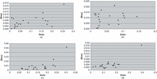
Graphs of the relationship between Δ and |bias| for 20 response propensity strata for (a) Hispanic ethnicity (correlation 0.55), (b) sex (correlation 0.16), (c) age (correlation 0.70) and (d) race (correlation 0.78)
7.2 Results for substantive variables
In addition to the screener variables, 10 substantive variables were analysed by using the same five models. These variables, which are listed in Table 2, were selected to represent a range of high and low prevalence characteristics that are essential to the NSDUH objectives. All the variables are intrinsically dichotomous. Unlike the screener variables, there are no natural gold standard estimates for these variables; therefore, it is not possible to assess bias accurately. Perhaps the best option for providing some indications of the non-ignorable non-response bias for these variables is to perform the tests of ignorability by propensity stratum that was described in Section 6.
Model 0 estimates of prevalence for the substantive variables and the bias estimated by the five models
| Variable† | Results (%) for the following models: | |||||
|---|---|---|---|---|---|---|
| Model 0 | Model 1 | Model 2 | Model 3 | GEM | ||
| ALCMON | 50.97 | −0.73 | −0.32 | −0.23 | −0.04 | 0.06 |
| ALCYR | 66.10 | −0.07 | −0.25 | −0.23 | 0.01 | 0.06 |
| CIGMON | 25.13 | −1.03 | −0.29 | −0.17 | −0.05 | 0.07 |
| COCMON | 0.98 | −1.48 | −0.22 | −0.13 | 0.00 | 0.14 |
| COCYR | 2.48 | −1.68 | −0.26 | −0.15 | 0.01 | 0.14 |
| MDELT | 13.90 | −1.40 | −0.12 | 0.00 | 0.02 | 0.07 |
| MDEYR | 7.43 | −1.73 | −0.06 | −0.03 | 0.06 | 0.09 |
| MJMON | 6.09 | −1.80 | −0.26 | −0.16 | 0.02 | 0.13 |
| MJYR | 10.34 | −1.76 | −0.32 | −0.19 | 0.01 | 0.12 |
| TOBMON | 29.70 | −1.02 | −0.31 | −0.18 | −0.08 | 0.07 |
ALCMON, past month use of alcohol; ALCYR, past year use of alcohol; CIGMON, past month use of cigarettes; COCMON, past month use of cocaine; COCYR, past year use of cocaine; MDELT, major depressive episode in lifetime; MDYR, major depressive episode in past year; MJMON, past month use of marijuana; MJYR, past year use of marijuana; TOBMON, past month use of tobacco.
Following the same approach as used for the screener variable analysis, 20 response propensity strata were formed on the basis of the GEM. In this analysis, the full GEM, including the four screener variables, was used to form the strata. If the GEM is successful at removing the bias for a substantive variable G, then the tests of ignorability for the variable G should not be rejected in any stratum. If the test is rejected for one or more strata, then there is at least some evidence that response propensity differs by the levels of G. This implies that the GEM does not adequately remove the non-ignorable non-response bias for this variable.
An overall measure of the adequacy of the GEM is the (weighted) average value of Δ for the 20 response propensity strata, which is denoted by , using weights that are proportional to the stratum size. The larger the value of , the greater the potential bias in the GEM estimator. To judge the magnitude of , we use results for the two dichotomous variables in the screener analysis: sex and Hispanic ethnicity. For these variables, is 0.05 and 0.09 respectively, and both variables have large biases whenever Δ exceeds 0.10. Thus, we consider larger than 0.10 to be an indication of problematic non-ignorable non-response bias in the GEM estimator. This cut-off value is chosen for illustration purposes only and may be inappropriate for general use. In practice, a simulation study could be performed to determine a cut-off value that is tailored to the specifics of the problem at hand.
The second column of Table 2 reports the unadjusted prevalence estimate from model 0 (i.e. . The remaining columns report the difference between this estimate and the model estimate (i.e. for the model in the column heading. This difference can be interpreted as an estimate of the non-response bias estimate of model 0 under model m for m≠0. These estimates were computed for 20 response propensity strata and then averaged over the strata weighting by the stratum size. The last column reports the value of for each variable.
Across all models, the differences are in the range from −2 to 0.1 percentage points, suggesting that underestimation may be the primary issue for these 10 variables. According to the model estimates, the biggest absolute biases are observed for model 1; however, model fit improves moving to model 2 and model 3, and the magnitude of the bias estimates tends to become smaller. In general, the GEM tends to report the smallest biases. This result combined with the result from the call-back model bias estimates suggests that the GEM estimates may be subject to non-ignorable non-response bias.
In Table 2, four variables have s that exceed 0.10—COCMON, COCYR, MRJMON and MRJYR—suggesting that non-ignorable non-response bias may be a problem for these variables. A large value of means that model 1 provides a substantial improvement in fit over model 0 and, further, that model 1 reduces the ignorable non-response bias that is ignored by the standard GEM adjustment. The GEM adjustment is quite small, which suggests that the GEM may not be effective at reducing the non-ignorable non-response bias for these variables. According to model 3, the biases are not small—e.g. −0.15 percentage points for past year cocaine use (COCYR) and −0.20 percentage points for past year marijuana use (MRJYR)—further suggesting that the GEM adjustment may not be effective.
8 Errors in the level-of-effort data and their effects
Table 1 suggests that the call-back models are misspecified in some way because a well-specified model should be more effective at removing the non-response bias. Adding more α- and β-parameters to the model, although improving model fit, did not reduce the bias in the prevalence estimates. As previously noted, an interesting phenomenon was observed regarding the β-parameters. Models that allowed the β-parameters to vary across the levels of G markedly improved the model fit, but the resulting estimates of πg were substantially more biased. Although the model misspecification may still be an issue, another possibility for these puzzling results is that the LOE data are contaminated by measurement errors that impart biases in the call-back model estimates.
A key assumption in call-back modelling is that the number of call attempts is recorded accurately. The model postulates that response propensity is a function of the number of attempts that are made to interview an individual. From the form of the estimator of πg in expression (5), it is apparent that small errors in the number of call-backs can potentially cause important biases in the estimates of πg. Therefore, understanding the quality of the LOE data is important to interpret the results of this research.
However, understanding how errors in the LOE data and other paradata affect their uses is an important issue in survey methodology. Uses of paradata are expanding (see, for example, Couper and Lyberg (2005)), particularly in the context of error modelling (see, for example, Beaumont (2005), Durrant and Steele (2009) and Heerwegh (2003)). It is generally acknowledged that the risk of error in paradata is high (Kreuter and Casas-Cordero, 2010; Wang and Biemer, 2010). Yet, rather surprisingly, we found no prior studies of the errors in LOE data, especially as they affect call-back model estimates. If modelling with LOE data is to progress, the issue of data errors and their effects should be studied.
To investigate the LOE data quality and its effects on the estimates of πg, two steps were taken. First, a field investigation of the processes that were used to collect the LOE data in the NSDUH was conducted. The results from this investigation were used to inform the error simulation models that were used to study the effects of LOE errors on the model estimates. A full report of the findings of the field investigation can be found in Wang and Biemer (2010). Here we briefly summarize the key results.
For our investigation of the types, frequencies and causes of LOE data errors, we asked all NSDUH interviewers to complete a questionnaire that explored their current reporting practices and how they handle specific situations in the field. The questionnaire requested information regarding how the LOE data are recorded and what factors might lead interviewers to record this information incorrectly. Additionally, interviewers were asked for suggestions to improve the LOE quality of the data and the process of collecting them. A total of 601 responses were obtained from 653 interviewers. In addition to the survey, focus groups were conducted with field supervisors, regional supervisors and regional directors to obtain their thoughts regarding sources of error in recording LOE data in the field.
The results of these data gathering efforts clearly indicated that LOE recording errors frequently occur that may be either unintentional or deliberate. Quite often, call-backs are misreported because the guidelines regarding what constitutes a call attempt can be ambiguous. For example, an interviewer may drive by a dwelling unit to look for indications that the respondent is at home (e.g. a car in the driveway or lights on in the house). However, if these ‘drive-by sightings’ suggest that no one is at home and so the interviewer never stops at the dwelling unit, interviewers were quite inconsistent regarding whether a call attempt should be recorded. Yet, by the interview guidelines, this situation would constitute a call attempt. Interviewers also acknowledged that they sometimes neglect to report call attempts to ‘keep a case alive’ because too many unproductive visits at a dwelling unit will cause the case to be closed. Although there were also suggestions that call-backs could be overreported, such errors occur much less frequently because they can be easily detected by supervisors who regularly inspect and check interviewer call records for signs of overbilling. These inquiries clearly indicated that the preponderance of errors appeared to be underreporting of call attempts, not overreporting.
On the basis of this study, it is plausible that errors in the LOE data, particularly underreporting of call-backs, are at least partially responsible for the disappointing performance of the call-back models in the NSDUH application. This possibility was further investigated in a simulation study where underreporting errors were created in the NSDUH LOE data to evaluate their biasing effects on the model estimates. As described next, a simple error model was used. For example, the model assumes that errors in the LOE data are independent—a seemingly unrealistic assumption given the above discussion regarding potential interviewer effects. Nevertheless, we believe that the findings are still useful for examining call-back model robustness and the nature of the bias caused by call-back underreporting errors. The key results are summarized here. Further details are reported in Biemer et al. (2011).
For the call-back underreporting error model, let udg denote the probability that the ath call attempt was not recorded for a unit in group g having disposition d and assume that udg is the same for all call attempts. Assume also that underreporting occurs independently, both within cases and between cases. These assumptions probably oversimplify the actual call-back error mechanism and, as reported in Biemer et al. (2011), models with somewhat greater complexity were explored but did not change our main conclusions.
Let denote the number of cases that are recorded with a attempts in disposition d and group g where nadg is the actual number of cases. Conditioning on nadg, the expected value of can be written as
where b(t,a,udg) is the zero-truncated binomial distribution with parameters t and udg at each attempt a and is given by
The distribution is zero truncated because at least one attempt must be recorded for every case in the sample.
For the results that are reported here, two levels of underreporting error (5% and 20%) were considered for three scenarios: underreporting occurs
- (a)
only for interviewed cases,
- (b)
only for refusal and non-contacted cases, and
- (c)
at the same rate for all cases.
Table 3 presents an example of the type of results that were obtained for this analysis. Our results assume a dichotomous variable with parameters πg=0.15, α1=0.4 and α2=0.5. To investigate the effects of varying the β-parameters across groups, we considered two cases: equal probabilities (i.e. and unequal probabilities (i.e. β1=0.75 and β2=0.85). The simulations were carried out by replacing nadg in the ADG-table by their corresponding conditional expected values, i.e. and fitting the correct model (i.e. model 1 for data where and model 1′ for data where .
Estimates of simulation population parameters under model 1 for 12 scenarios
| Error rate applied to | udg | for the following values of β1 and β2 : | |
|---|---|---|---|
| Interviewed cases only | 0.050 | 0.151 | 0.179 |
| Refusal or non-contacted cases only | 0.050 | 0.150 | 0.126 |
| All cases | 0.050 | 0.150 | 0.151 |
| Interviewed cases only | 0.200 | 0.152 | 0.276 |
| Refusal or non-contacted cases only | 0.200 | 0.148 | 0.113 |
| All cases | 0.200 | 0.150 | 0.152 |
As shown in Table 3, the effects of underreporting errors on the estimates of π1 are fairly small when the true model imposes the constraint , even when the level of underreporting is as high as 20%. This is true whether or not the error level is dependent on the disposition. Not shown in Table 3 are the estimates of contact and interview probabilities— and β2—which have much larger biases.
The more interesting case is when the true model specifies and this model is also fitted to the simulated data. In these simulations, even small levels of underreporting errors had substantial effects on the estimates of πg. For example, in Table 3, when the underreporting rate is only 5% for interviewees (and 0% for refusals), the bias is 0.179 – 0.150 = 0.029; a relative bias of about 19%. Likewise, when the underreporting rate is 5% for refusals and non-contacts and 0% for interviews, the bias changes direction and is smaller; but it is still substantial, with a relative bias of about −16%. These effects are magnified as the error rates increase. At a 20% error rate, the relative bias is 84% and −25% respectively, for the two types of error. Interestingly, when the error rate is the same for all dispositions, the bias was negligible, even at the higher level.
The analysis was repeated with various alternative configurations of the model parameters and the results were essentially the same. Likewise, the simulations were repeated, allowing the rate of underreporting to vary by G, again with the same results. The estimates of πg under model 1 are fairly robust to call-back data errors. Under model 1′, however, errors that depend on the case disposition or the outcome variable can cause substantial biases in the estimates of πg. When errors are independent of both G and D, both models 1 and 1′ performed well. LOE error rates that vary by level G (or D) can cause artificial discrepancies in the mean response propensities by level which in turn will exaggerate the magnitudes of non-response biases.
These results mirror our experience in applying these models to the NSDUH data. The models that specified performed much better than the corresponding models with this constraint removed. However, the models specifying were still somewhat biased, probably as a result of being misspecified, because for many characteristics, including the screening variables in our evaluation, interview probabilities are likely to vary by the levels of G.
9 Conclusions
This paper extends the work of Biemer and Link (2007) to address the additional complexities that are encountered in the application of call-back models to field surveys. A new indicator, which was denoted by Δ, was proposed as a possible indicator of the non-ignorable bias remaining in an estimate. The extended call-back model and non-ignorability measure were both applied to data from a large-scale field survey. The results suggest that Δ may be useful for its intended purposes; however, the call-back model did not perform as well as the traditional response propensity adjustment approach that is currently used in the survey. The GEM adjustment, with the G (a screener variable) removed (denoted by model 0), was better at adjusting for the non-response bias in G than were the call-back models.
After trying a wide range of more elaborate call-back models, we suspected that the lacklustre performance of the call-back model was related to the quality of the LOE data, not model misspecification. A fairly extensive investigation into the possible sources and causes of LOE data errors confirmed our suspicions. Underreporting of call attempts occurs in field surveys and these errors can be detrimental to call-back model performance, particularly when the rates of underreporting depend on the case disposition or the outcome variable. More studies of these and other paradata errors are clearly warranted.
Using a simple zero-truncated binomial model, underreporting error was simulated for the LOE data from the survey. These simulations suggest that LOE data errors are not particularly problematic unless the errors are correlated with either G or the dispositions D. Even then, call-back models that constrained the β-parameters across groups are fairly robust to these errors. The problem arises when the β-parameters vary across groups. These symptoms were manifest in our NSDUH application. Models that allowed the β-parameters to vary by G were extremely biased and abandoned, whereas models that constrained these parameters performed much better. The models that specified for all g and g′ (i.e. models 0, 1, 2 and 3) were still somewhat biased; however, in this case model misspecification (from imposing the equality constraint) may contribute more bias than LOE data error.
Biemer and Link (2007) reported much better success with the call-back modelling approach in their application to the ‘Behavior risk factor surveillance system’—a national RDD survey. However, call-back data could be of much greater quality in this survey, and in RDD surveys in general, because of the controls in place for recording call attempts and their outcomes for each dialled number. In addition, in Biemer and Link’s (2007) study, the call-back model was competing with a somewhat ineffective post-stratification adjustment approach for adjusting for non-response bias in the ‘Behavior risk factor surveillance system’. In that situation, the call-back model provided a marked improvement in bias reduction. By contrast, the NSDUH GEM uses a considerable amount of data that are available at the household level. It should be no surprise that adding an LOE variable to this extensive amount of data showed much less improvement.
It may be possible somehow to incorporate an error term in the call-back modelling approach to correct for underreporting error. However, given the potential complexity of these errors, modelling them is ostensibly not a viable option. A more successful approach may be to introduce changes in the data collection process to enhance the quality of the call-back data. However, given the potential burden on the field interviewers that could result from these changes, the cost and benefits of obtaining highly accurate LOE data should be carefully considered.
Acknowledgements
The authors gratefully acknowledge the US Substance Abuse and Mental Health Services Administration, Office of Applied Studies, who provided partial support for this research under contract 283-2004-00022 and project 0209009. The views expressed herein are those of the authors and do not necessarily reflect the official position or policy of the US Department of Health and Human Services.
