


Abstract
This study aimed to develop and validate a collapsed cone convolution for magnetic resonance-guided radiotherapy (CCCMR). The 3D energy deposition kernels (EDKs) were generated in water in a 1.5-T transverse magnetic field. The CCCMR corrects the inhomogeneity in simulation geometry by referring to the EDKs according to the mass density between the interaction and energy deposition points in addition to density scaling. Dose distributions in a water phantom and in slab phantoms with inserted inhomogeneities were calculated using the Monte Carlo (MC) and CCCMR. The percentage depth dose (PDD) and off-axis ratio (OAR) were compared, and the gamma passing rate (3%/2 mm) was evaluated. The CCCMR simulated asymmetric dose distributions in the simulation phantoms, especially the water phantom, and all PDD and OAR profiles were in good agreement with the findings of the MC. The gamma passing rates were >99% for each field size and for the entire region. In the inhomogeneity phantoms, although the CCCMR underestimated dose in the low mass density regions, it could reconstruct dose changes at mass density boundaries. The gamma passing rate for the entire region was >95% for the field size of 2 × 2 cm2, but it was 68.9–86.7% for the field sizes of ≥5 × 5 cm2. Conclusively, in water, the CCCMR can obtain dose distributions comparable to those with the MC. Although the dose differences between them were mainly in inhomogeneity regions, the possibility of the effective use of the CCCMR in small field sizes was demonstrated.
INTRODUCTION
Magnetic resonance (MR)-guided radiotherapy (MRgRT) was developed to improve treatment accuracy, and MR images are used to reduce setup uncertainty without additional imaging dose. Because MR images provide high soft tissue contrast, MRgRT can directly localize the tumor [1]. Furthermore, MR images have been used to monitor treatment response and biological or functional images [2, 3]. MRgRT systems allow online adaptive radiation therapy (online-ART) for treatment adjustment according to the conditions of tumor volume or the organs at risk based on pretreatment assessment [4, 5].
Treatment planning systems for MRgRT use Monte Carlo (MC) simulation to obtain the dose distributions in magnetic fields because MC simulation can accurately simulate particle transport in a magnetic field [6, 7]. One of the drawbacks of MC simulation is that it requires a long calculation time to obtain sufficient statistical significance; however, it is becoming clinically acceptable. Although MC simulation uses variance reduction techniques and a graphical processing unit (GPU) to reduce the calculation time, a certain calculation time is required to obtain the dose distribution if the optimization step of intensity-modulated radiation therapy (IMRT) is included [8]. Some researchers revealed the planning time for online-ART in MRgRT. Raaymakers et al. reported that Unity 1.5 T (Elekta AB, Sweden) requires ~ 5 min for their concept, and Acharya et al. showed that the median ART time for MRIdian (Viewray, Inc, Cleveland, OH) was 26 min, including the recontouring, reoptimization and QA steps [4, 9]. Moreover, Muinck Keizer et al. reported that patients with prostate diseases had an average on-couch time of 40 min during a single fraction, and targets, such as the prostate and seminal vesicle, had intrafraction motion of a few millimeters 10 min after the first cine-MR dynamic image acquired in that fraction [10]. Circumstances should be created to allow the immediate start of treatment beam irradiation after imaging or creating a treatment plan on online-ART to reduce variations in the patient’s body.
Collapsed cone convolution (CCC)/superposition dose calculation algorithms that use the precalculated energy deposition kernels (EDKs) by MC simulation can obtain dose distributions faster than MC methods because of the amount of computation. Furthermore, CCC algorithms can obtain the dose distributions within a few seconds with the use of GPUs [11, 12]. If CCC algorithms could be applied to MRgRT, we would be able to reduce the patient’s waiting time associated with dose calculation as well as improve the intra-fractional errors. The major difference from the conventional situation without a magnetic field is that it is necessary to reproduce the dose variations caused by the Lorentz force in a magnetic field. In particular, the direction of the field is orthogonal to the treatment beam, and non-negligible dose changes are caused by the electron return effect (ERE) at mass density change regions, such as the body surface and hollow organs [13]. General CCC algorithms assume that the human body is constructed with water and calculated the dose to water. The EDK obtained in water is discretized into a cone shape with the origin at the interaction point to reduce the amount of calculation and achieve high speed. Moreover, inhomogeneity correction is performed by scaling the length based on the mass density on the path of each cone [14]. EDKs were acquired not in water but in arbitrary body tissues and materials (material-specific kernel) and used for CCC algorithms to improve the dose calculation accuracy in not only in the MV domain but also in the kV domain [15, 16]. The use of EDKs obtained from arbitrary materials improves dose calculation accuracy because the reproducibility of particle transport in arbitrary materials can be improved.
In this study, we generated EDKs obtained from water with varying mass densities (mass-specific EDK [EDKms]) to consider that the trajectory of particles in a magnetic field varies with the mass density of water. We attempted to obtain the dose distributions in a transverse magnetic field by using the CCC algorithm with EDKms and validated the accuracy of the CCC algorithm with EDKms compared with MC dose distributions.
MATERIALS AND METHODS
Generation of the EDKms in a magnetic field
MC code Electron Gamma Shower version 5 (EGS5) was used to obtain EDKs in a magnetic field, and the accuracy of this process in a magnetic field was evaluated according to the method by Ito et al. [17]. We used a homogeneous sphere of water with a radius of 60 g·cm−2 to obtain EDKs. The radial boundaries of voxels were defined at the intersection of 65 radial shells. The smallest radial spacing was 0.01 g·cm−2, which occurs immediately surrounding the origin, and the largest radial spacing was 5.0 g·cm−2, which occurs near the edge of the phantom. As a high-dose gradient would be observed near the site of the incident photon, high-resolution scoring boundaries were defined. Conversely, as a roughly equal amount of energy deposition would be observed on the distal side in the phantom, low-resolution scoring boundaries were defined. Generally, the CCC method uses the kernels obtained by discretizing the 3D EDKs into 2D polar coordinates, since a symmetrical point spread dose distribution is produced in the homogeneous media without a magnetic field. However, the EDKs in a magnetic field are expected to be distorted and affected by the Lorentz force depending on the relationship between the direction of the incident primary photon and the magnetic field. In addition, it is straightforward to assume that the reconstruction of the distorted dose distribution in a magnetic field from 2D general EDKs is extremely challenging. Hence, to be able to consider the distorted EDKs in a magnetic field, the angular boundaries (Ω) were defined by dividing 4π steradian (sr) into 0.0086 sr (=6°) to construct 3D distorted EDKs. Figure 1 shows a schematic of the simulation geometry.
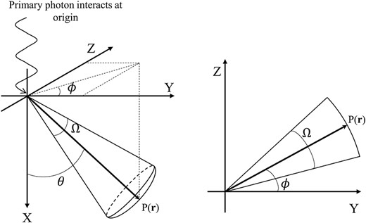
Schematic of the coordinate system for the generation of EDKs in a magnetic field. Monoenergetic primary photons interact at the origin, which is the center of the water sphere. P(r) indicates the position of the particle, and θ and ϕ are the angles between the vector r and the positive X or Y axis. Ω is the angular boundary as the steradian.
Water has a mass density of 1 g·cm−3 under standard conditions. In this study, to consider that the trajectory of the charged particle is dependent on the mass density of the medium in the pathway, we obtained EDKs generated in the water sphere, which had a mass density of 0.25 g·cm−3 at intervals between 0.25 and 2.0 g·cm−3. Hence, eight EDKs were obtained per monoenergetic primary photon. The generated EDKs were specific to the mass density of water; hence, we defined them as EDKsms. The radii of the water spheres were scaled based on the mass density of each simulation so that the product of the radius and mass density was the same for all simulations (e.g. r1.0 × ρ1.0 = r0.25 × ρ0.25; subscripts mean the mass density [g·cm−3]). The monoenergetic EDKsms from 1.0 to 7.0 MeV were obtained at 1.0 MeV intervals. The strength of the magnetic field was set to 1.5 T, and the direction of the field was perpendicular to the incident primary photon direction. The relationship between the direction of the primary photon and the field assumed that the treatment beam and field direction are orthogonal in MRgRT.
The history number was set to 1 × 10⁸ to generate each EDKms. The EDKms and statistical uncertainty of the MC simulation were determined for each calculated quantity by dividing the calculations into 10 batches and computing the mean and root mean square deviation from the mean from these 10 values. Furthermore, to characterize the variation in the EDKms depending on the mass density, the effective depth (|$\overline{z}$|), effective radial distance (|$\overline{r}$|) and effective lateral distance (|$\overline{y}$|) were obtained for each EDKms. These parameters explained the average traveling distance of the charged particle from the interaction point.
The effective radial distance |$\overline{r}$| is described as follows:
where |${\varepsilon}_{\mathrm{prim}}\left(i,j\right)$| is the energy deposition of the primary charged particle of the i, jth voxel. Furthermore, the effective radius of each voxel |${\hat{r}}_{\mathrm{prim}}\left(i,j\right)$| by the primary charged particle is described as follows:
where rn is the distance from the origin of the sphere to the center of the i, jth voxel, and n is the number of MC iterations. The effective depth |$\overline{z}$| is described as follows:
where |${\hat{z}}_{\mathrm{prim}}\left(i,j\right)$| is the effective depth of each i, jth voxel by the primary charged particle, which is described as follows:
where |$\cos \big[{\hat{\theta}}_{\mathrm{prim}}\left(i,j\right)\big]$| is the cosine value of the effective angle |${\hat{\theta}}_{\mathrm{prim}}\left(i,j\right)$| of each i, jth voxel by the primary charged particle, which is the angle between the direction of the incident primary photon and the middle of the voxel of the particle position. The effective lateral distance |$\overline{y}$| is obtained from |$\overline{r}$| and |$\overline{z}$|, and is described as follows:
The ratio of |$\overline{z}/\overline{y}$|, which indicates whether the charged particles deposit their energy in the forward or lateral direction, and the shape of the EDKms were obtained [15, 16, 18]. The cutoff energies for photons and electrons were set to 0.01 and 0.521 MeV, respectively. The EFRACH/EFRACL variables, which specify the fractional energy losses over multiple scattering steps at the highest or lowest problem energies, respectively, were set at 0.02. The maximum user step length (‘mxustep’) of the charged particles was set to 0.001 cm.
CCC/superposition dose calculation algorithm and inhomogeneity correction
The original convolution/superposition dose calculation (C/S) algorithm was expressed using the following equation:
where r is a point at which a dose is calculated, and s is the source point of the energy imparted to r. TE indicates the total energy released by primary photon interactions per unit mass (TERMA) and is expressed as follows:
where |$\mu /\rho \left(E,\mathbf{r}\right)$| is the mass attenuation coefficient of the primary photons of energy E at point r, and |${\Phi}_E\left(\mathbf{r}\right)$| is the primary photon fluence differential in energy at r. Because the photon attenuation is not affected by a magnetic field, the TERMA distribution can be obtained using the general method. We assumed that the TERMA is constant in one voxel because the TERMA usually varies slowly [19]. In addition, |${h}_{\rho_0}$| indicates the point spread EDK in a homogeneous medium of density |${\rho}_0$|. The vector (r–s) is rescaled according to the mass density on each path length to consider inhomogeneous correction [14]. The CCC algorithm is an approximation of the C/S algorithm and uses the EDK that is collapsed to a discrete number of directions. The complexity of the CCC algorithm is O(N4M) for arbitrary EDK, where M is the number of collapsed cone directions with inhomogeneity correction, whereas that of the C/S algorithm is O(N7), which is significantly more than that of the CCC algorithm [20]. As the CCC algorithm requires less calculation, it can quickly obtain the dose distributions.
In addition to the radiological path length from s to r (|${p}_{\mathbf{s},\mathbf{r}}$|), the CCC algorithm developed by us for MRgRT (collapsed cone convolution for magnetic resonance-guided radiotherapy [CCCMR] algorithm) obtained the average mass density from s to r (|${\overline{\rho}}_{\mathbf{s},\mathbf{r}}$|) for the inhomogeneity correction. The energy deposition from s to r was obtained from the EDKms(|${\overline{\rho}}_{\mathbf{s},\mathbf{r}},{p}_{\mathbf{s},\mathbf{r}}$|) generated in a water sphere with mass density |${\overline{\rho}}_{\mathbf{s},\mathbf{r}}$|. In case EDKms(|${\overline{\rho}}_{\mathbf{s},\mathbf{r}}$|) was not generated, the CCCMR algorithm obtained the EDKms(|${\overline{\rho}}_{\mathbf{s},\mathbf{r}}$|) by linear interpolation between EDKms(|${\rho}_i$|) and EDKms(|${\rho}_j$|) (|${\rho}_i<{\overline{\rho}}_{\mathbf{s},\mathbf{r}}<{\rho}_j,$|i or j = 0.25, 0.5, …, 2.0 g·cm−3). For instance, if the average mass density from s to r was 0.33 g·cm−3, the CCCMR algorithm referred to the EDKms(0.33) interpolated from the EDKs generated in the water sphere that had a density of 0.25 and 0.5 g·cm−3, and the energy deposition was obtained from the point ps, r in the interpolated EDKms(0.33).
Furthermore, the CCCMR algorithm can be rewritten from Equation (7) as follows:
where |${\mathrm{EDK}}_{\mathrm{ms}}\left(E,{\overline{\rho}}_{\mathbf{s},\mathbf{r}},{p}_{\mathbf{s},\mathbf{r}}\right)$| is the EDKms at the ps, r of primary photon energy E obtained in the water sphere of mass density |${\overline{\rho}}_{\mathbf{s},\mathbf{r}}$|. The schematic of the inhomogeneity correction in the CCCMR algorithm is shown in Fig. 2. Our developed CCCMR algorithm was described by FORTRAN and used Open-MPI to achieve parallel computation on a Central Processing Unit.
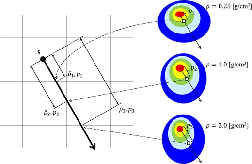
The schematic of the inhomogeneity correction in the CCCMR algorithm. The left image shows the volume segment, and the right image shows the EDKms generated in each arbitrary mass density. s is the interaction point, and the thick arrow from s indicates the energy transportation direction. |${\overline{\rho}}_i$| and |${p}_i$| (i = 1, 2, 3) indicate the average mass density and the radiological path length from s to each cross plane, respectively. The image shows cases where |${\overline{\rho}}_1$|, |${\overline{\rho}}_2$| and |${\overline{\rho}}_3$| are equal to 0.25, 1.0 and 2.0 g·cm−3, respectively. The energy depositions from s to |${p}_1$|, |${p}_2$| and |${p}_3$| are obtained from |${p}_1$|, |${p}_2$| and |${p}_3$| in the EDKsms generated at 0.25, 1.0 and 2.0 g·cm−3, respectively. When the EDKms is not preobtained for the mass density corresponding to |${\overline{\rho}}_i$|, the EDKms corresponding to that mass density is calculated by linear interpolation and is used to obtain the energy deposition. In inhomogeneity correction in the CCCMR algorithm, the referenced EDKms is determined or interpolated according to the average mass density from the interaction point to the calculation point.
Validation of the accuracy of inhomogeneity correction by density scaling
The CCCMR algorithm proposed in this study uses density scaling and reference to EDKms according to the average mass density between interaction and dose calculation points as the inhomogeneity correction. The accuracy of the inhomogeneity correction was validated by comparing the dose distributions and profiles of spherical phantom obtained from the MC and CCCMR. The phantom was filled with water, and a 1-cm thick low mass density (0.25 [g/cm3]) slab was inserted at a depth of 0.5–1.5 cm. The dose distributions were obtained by interacting the primary photon 4 MeV at the center of sphere.
Validation of the CCCMR algorithm by comparison with the MC simulation
In this study, three different virtual phantoms were used, each having dimensions of 21.0 × 15.4 × 15.4 cm3 with a voxel size of 0.2 cm. The schematic of the phantoms is shown in Fig. 3. One phantom was water-filled and homogeneous, and two were heterogeneous and comprised lung and bone slabs and a spherical tumor having a diameter of 2 cm. The mass densities of the water and tumor, the lung and the bone were 1, 0.33 and 1.92 g·cm−3, respectively.
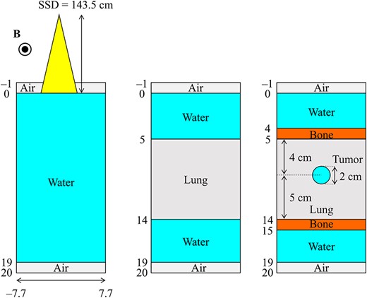
Schematic representation of phantom geometries. The left image shows the homogeneous water phantom, the center image shows the slab lung and water phantom and the right image shows the slab lung and bone phantom with an inserted spherical tumor.
Reference dose distributions were obtained from EGS5. As our proposed CCCMR algorithm calculates dose to water (Dw) by using the EDKms generated in water, EGS5 also calculates Dw. Dw was obtained using water as the medium in EGS5 and setting only the mass density as described above. The settings of the MC simulation, such as cutoff energy, EFRACH/EFRACL and field direction and strength, were similar for EDKms generation.
The source-to-surface distance and field sizes were set to 143.5 cm and 2 × 2, 5 × 5 and 10 × 10 cm2, respectively, at the phantom surface. The history number was set to 1 × 10⁹ for 2 × 2 and 5 × 5 cm2 and 2 × 10⁹ for 10 × 10 cm2. Variance reduction techniques to reduce the statistical uncertainty of the MC simulation were not used in our study. A point source was used to generate a photon beam composed of the Unity energy spectrum for MC calculations [6]. For the CCCMR calculations, the energy spectrum was determined to produce the same percentage depth dose (PDD) curve as the PDD curve in the water phantom obtained from the MC calculation, and all CCCMR calculations were performed using this energy spectrum with a point source. Neither the MC nor CCCMR calculations considered varying the energy spectrum in the off-axis direction. All dose distributions obtained from both algorithms were normalized by the maximum dose point on the central axis (CAX) for each field size in the water phantom.
Volumetric dose comparison was performed using a 3D gamma test [21]. Furthermore, MATLAB software (MathWorks, Natick, MA), which was created by Mark Geurts (https://github.com/mwgeurts/gamma), was used to perform gamma analysis. The gamma index for each voxel at r is defined as follows:
where |${\mathbf{r}}_{\mathrm{MC}}$| and |${\mathbf{r}}_{{\mathrm{CCC}}_{\mathrm{MR}}}$| represent the position vectors for the reference (MC simulation) and evaluated (CCCMR algorithm) distributions, respectively, and D represents the dose at each point. ∆d and ∆D are the distance to agreement (DTA) and dose difference criteria, respectively. Gamma values less than or equal to 1 and those greater than 1 indicate that the comparison passed and failed, respectively. The baseline criteria for ∆d and ∆D were 2 mm and 3%, respectively. As our comparisons were all between simulated doses, a tolerance of DTA 2 mm, which corresponds to one voxel size, was set. Gamma tests were performed for not only the entire volume, but also for each subregion of the dose distribution, which was divided into the buildup region, penumbra region and inner region, as in AAPM TG-53 definitions [22]. The buildup region corresponded to the voxels located from the surface to the depth of maximum dose (dmax). The penumbra region corresponded to the voxels with doses between 20 and 80% of the CAX MC dose. The inner region corresponded to the voxels with doses greater than 80% of the CAX MC dose. The agreement between both algorithms was evaluated by the gamma passing rate, which was calculated by the ratio of the number of passing voxel to the total volume of each region.
All MC and CCCMR simulations were performed in parallel on 40 cores. MC simulations were performed with different random number seeds on each core. A PC with two Intel Xeon Silver 4116 processors (2.1 GHz, 12 cores) was adopted for dose calculation, using the CCCMR algorithm and MC simulation, and the calculation time was compared.
RESULTS
Figure 4 shows the EDKs within 5 g·cm−2 from the origin at 4.0 MeV in 0.25, 1.0 and 2.0 g·cm−3 water in the XY plane as shown in Fig. 1. The asymmetric EDKs were reconstructed, and the shape of the kernels varied with the mass density of water.
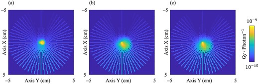
Generated 3D EDK of the primary photon energy at 4 MeV in the XY plane at the origin as shown in Fig. 1. The primary photon interacts at the center of the image. (a–c) show the EDKs generated in 0.25, 1.0 and 2.0 g·cm−3 water, respectively. WW, 10−15–10−9 Gy photon−1.
In Fig. 5, the parameters characterizing the EDKms, the effective depth (|$\overline{z}$|), the effective radial distance (|$\overline{r}$|), the effective lateral distance (|$\overline{y}$|) and the ratio of |$\overline{z}/\overline{y}$| are presented in each mass density of water at the primary photon energy from 1.0 to 7.0 MeV. The statistical uncertainties of the MC simulation were smaller than the plot markers and were not visible on the graphs. The effective depth and range increased as a function of the mass density. For the effective lateral distance, the curves produced a peak of ~0.75–1.0 g·cm−3. The ratio of |$\overline{z}/\overline{y}$| indicated the direction in which charged particles deposited their energy in the medium. The EDKms was distorted to the left and right when the density was low and elongated vertically as the density increased.

Comparison of the (a) effective depth, (b) effective radial distance, (c) effective lateral distance and (d) ratio of z/y in each mass density of water and at each primary photon energy. The statistical uncertainties of the MC simulation were smaller than the plot markers and were not visible on the graphs.
Figure 6 shows the dose distribution and profile obtained from the MC and CCCMR in the spherical water phantom. In Fig. 6a, the isodose lines of the MC and CCCMR are indicated by solid and dashed lines, respectively. Figure 6b shows the MC and CCCMR dose profiles at 0°, 42° and 90° relative to the direction of the primary photon with solid and dashed lines, respectively. The dose profiles of the CCCMR and MC were consistent in the 0° direction, but the CCCMR overestimated and underestimated one of the MCs in the 42° and 90° directions, respectively.
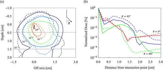
Incorporating a low mass density slab into the spherical water phantom allowed for a comparison of the inhomogeneity corrections of the MC and CCCMR. A comparison of the (a) dose distributions and (b) dose profiles, respectively. In the area enclosed by the dashed line in (a), a slab of low mass density is inserted. The MC and CCCMR calculations are represented by solid and dashed lines, respectively. Dose distributions were normalized at the dose of primary photon interaction point (0, 0) in (a), and isodose lines are shown at 100, 10−1, 10−2, 10−3 and 10−4. The dose profiles at 0°, 42° and 90° to the direction of the primary photon are depicted.
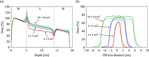
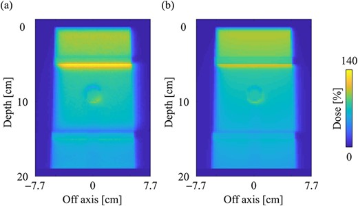
Figure 7a and b shows the dose distributions obtained from the MC and CCCMR with the field size of 10 × 10 cm2 in the water phantom, respectively. All dose distributions were normalized at the maximum dose point in the water phantom. Figure 8a and b shows the PDD curves at the CAX and the off-axis ratio (OAR) profiles at a depth of 9 cm obtained from both the MC and CCCMR for each field size. Red, blue and green colors indicate the results for field sizes of 2 × 2, 5 × 5 and 10 × 10 cm2, respectively. Solid and dashed lines indicate the MC and CCCMR results, respectively. All PDD curves obtained from the CCCMR algorithm were in agreement with the MC curves, and the average differences from the MC simulation downstream of dmax were at the most 1.2%. The CCCMR algorithm can simulate the left–right distorted asymmetry dose distributions that are characteristic of the transverse magnetic field, as shown in the OAR profiles. The average difference was between 1.8 and 4.3% in the inner of the full width at half maximum.
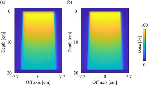
Dose distributions in the water phantom in the central slice obtained from the (a) MC and (b) CCCMR techniques, respectively. Dose distributions were normalized by the maximum dose point on the CAX for each algorithm, and the same points were used for the normalization of other simulation phantoms. The field size was set to 10 × 10 cm2 at the phantom surface.
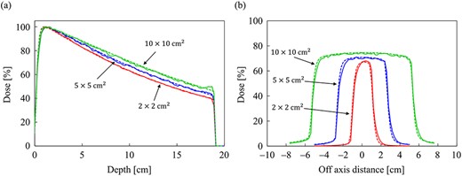
Comparison of (a) the PDD curves at the CAX and (b) off-axis profiles at a depth of 9 cm for the field sizes of 2 × 2, 5 × 5 and 10 × 10 cm2 in the water phantom. The solid and dash lines show MC and CCCMR calculations, respectively.
Figure 9a and b shows the dose distributions obtained from the MC and CCCMR with the field size of 10 × 10 cm2 in the slab lung phantom. The CCCMR algorithm can simulate hot and cold spots caused by changing the electron trajectories at the mass density boundaries, similar to that with MC simulation. Figure 10a and b shows the PDD curves at the CAX and the OAR profiles at a depth of 9 cm in the lung obtained from both MC and CCCMR for each field size. Red, blue and green colors indicate that the field sizes were 2 × 2, 5 × 5 and 10 × 10 cm2, respectively. The results of the MC and CCCMR were represented by dashed lines and solid lines, respectively. Although the CCCMR algorithm calculated the PDD curves consistent with the MC simulation in the water, the trend in the lungs differed depending on the field size. In the lung, the CCCMR algorithm calculated the same dose as the MC simulation for the field size of 2 × 2 cm2, whereas it underestimated the dose by 10% for the field sizes of 5 × 5 and 10 × 10 cm2. The OAR profiles also showed underestimation within the irradiation field in the lung. The CCCMR algorithm also underestimated the hot and cold spots occurring in the water/lung boundaries relative to the MC simulation.
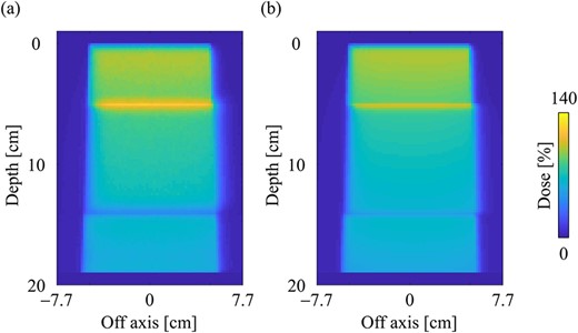
Dose distributions in the slab lung phantom in the central slice obtained from the (a) MC and (b) CCCMR techniques, respectively. Dose distributions were normalized by the maximum dose point on the CAX in the water phantom. The field size was set to 10 × 10 cm2 at the phantom surface.
Comparison of (a) the PDD curves at the CAX and (b) off-axis profiles at a depth of 9 cm for the field sizes of 2 × 2, 5 × 5 and 10 × 10 cm2 in the slab lung phantom. The abbreviations W and L in (a) stand for water and lung, respectively. The solid and dash lines show MC and CCCMR calculations, respectively.
The dose distributions obtained from the MC and CCCMR with the field size of 10 × 10 cm2 in a slab phantom inserted with a spherical tumor are depicted in Fig. 11a and b, respectively. The CCCMR algorithm can simulate the dose changes at the mass density boundaries, similar to that with the MC simulation. The PDD curves at the CAX and the OAR profiles at a depth of 9 cm (the center of the tumor) obtained from the MC and CCCMR at each field size are depicted in Fig. 12a and b, respectively. The results for a field size of 2 × 2, 5 × 5 and 10 × 10 cm2 were represented by the colors red, blue and green, respectively. Moreover, the results of the MC and CCCMR were represented by dashed lines and solid lines, respectively. The abbreviations W, B, L and T in Fig. 12 represent water, bone, lung and tumor, respectively. The PDD curves showed similar results to those of the slab lung phantom in the lung region of the spherical tumor phantom, with the CCCMR and MC doses agreeing in the field size of 2 × 2 cm2, but showing an underestimation of close to 10% with the other field sizes. In bone and tumor regions, the CCCMR algorithm underestimated the dose relative to the MC simulation regardless of the field size.
Dose distributions in the spherical tumor-inserted slab phantom in the central slice obtained from the (a) MC and (b) CCCMR techniques, respectively. Dose distributions were normalized by the maximum dose point on the CAX in the water phantom. The field size was set to 10 × 10 cm2 at the phantom surface.
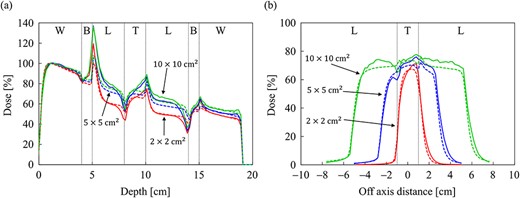
Comparison of (a) the PDD curves at the CAX and (b) off-axis profiles at a depth of 9 cm for the field sizes of 2 × 2, 5 × 5 and 10 × 10 cm2 in the spherical tumor-inserted slab phantom. The abbreviations W, B, L and T in (a) and (b) stand for water, bone, lung and tumor, respectively. The solid and dash lines show MC and CCCMR calculations, respectively.
The gamma distributions of the central plane for the water, slab lung and spherical tumor-inserted slab phantom are depicted in Fig. 13a–c, respectively, with a field size of 10 × 10 cm2. There was a notable number of voxels in the bone and lung regions in the inhomogeneity phantoms, and the findings did not pass the 3%/2 mm gamma criterion. Table 1 shows the gamma passing rate for each phantom, field size and subregion. In the water phantom, the gamma passing rates were >99%, regardless of the field size, in all regions, except for the buildup region. In the inhomogeneity phantoms, the gamma passing rates were > 90% in the buildup and penumbra regions, but 58.92–97.64% in the inner regions. Differences occurred mainly in the bone and lung regions, as shown by the dose profiles and gamma distributions.
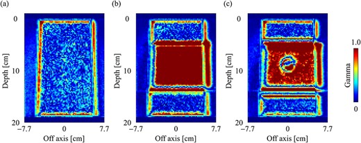
Gamma distribution (3%/2 mm) of dose distributions with the field size of 10 × 10 cm2 in the central slice for (a) water, (b) slab lung and (c) spherical tumor-inserted slab phantom.
The percentage passing rate of 3D gamma indices in the three phantoms for each subregion and field size; the criteria of dose difference and DTA were set to 3% and 2 mm, respectively
| Field size (cm2) | ||||
|---|---|---|---|---|
| Phantom | Subregion | 2 × 2 | 5 × 5 | 10 × 10 |
| Water | Buildup | 100.0 | 93.8 | 97.6 |
| Penumbra | 100.00 | 99.5 | 99.7 | |
| Inner | 100.00 | 99.6 | 99.9 | |
| All | 99.9 | 99.2 | 99.7 | |
| Slab lung | Buildup | 98.7 | 98.2 | 98.7 |
| Penumbra | 97.4 | 95.7 | 93.7 | |
| Inner | 97.6 | 69.8 | 58.9 | |
| All | 97.5 | 80.2 | 68.9 | |
| Spherical tumor | Buildup | 98.9 | 97.8 | 98.1 |
| Penumbra | 98.0 | 96.0 | 93.6 | |
| Inner | 93.9 | 80.8 | 76.0 | |
| All | 96.1 | 86.7 | 81.2 | |
The comparison of the computation time between the MC simulation and CCCMR algorithm is shown in Table 2. Speed increases due to the use of the CCCMR algorithm were ~150–1900 times depending on the field size.
Comparison of the computation times between the MC and CCCMR techniques in the three phantoms; the unit of time is minutes
| Phantom | Field size (cm2) | MC | CCCMR | Speed increase |
|---|---|---|---|---|
| Water | 2 × 2 | 1118.6 | 1.2 | ×908 |
| 5 × 5 | 1101.5 | 6.7 | ×165 | |
| 10 × 10 | 10 793.4 | 33.1 | ×326 | |
| Slab lung | 2 × 2 | 1099.4 | 1.1 | ×980 |
| 5 × 5 | 1106.8 | 6.1 | ×182 | |
| 10 × 10 | 10 779.1 | 30.6 | ×353 | |
| Spherical tumor | 2 × 2 | 2225.8 | 1.2 | ×1906 |
| 5 × 5 | 2226.8 | 6.3 | ×354 | |
| 10 × 10 | 10 786.9 | 31.4 | ×344 |
DISCUSSION
Generally, in the CCC algorithm without a magnetic field, the algorithm uses an EDK for each energy, which is generated in water with a mass density of 1 g·cm−3 and considers inhomogeneity correction by applying density scaling for each ray. In a transverse magnetic field, the trajectory of the charged particles varies due to the change in the mass density, as described above, distorting EDKs and dose distributions. To reproduce this phenomenon in the CCC algorithm, first, we generated the distorted EDKs in water with various mass densities (EDKms) in a transverse magnetic field. Second, the energy deposition to each point was determined by referring to the EDKsms according to the average mass density from the interaction point to the calculation point. In addition, if necessary, the EDKms corresponding to the average mass density was obtained by interpolation and applied to the dose calculations.
The CCCMR algorithm proposed in this study can calculate the dose distribution with left–right distortion that is characteristic of the transverse magnetic fields by applying EDKsms. Furthermore, although the CCCMR algorithm was able to reproduce the dose change caused by the abrupt change in electron trajectories at the mass density boundaries, the dose change was underestimated relative to the MC simulation. The gamma passing rates (3%/2 mm) in the water phantom were greater than 99% for all field sizes in all regions, except the buildup region, indicating that the CCCMR algorithm can calculate dose distributions consistent with the MC simulation in homogeneity regions. The CCCMR algorithm underestimated the dose by 10% in the low mass density region for larger field sizes, markedly reducing the gamma passing rate. However, the CCCMR algorithm calculated the doses consistent with the MC simulation even in the low mass density region for the field size of 2 × 2 cm2, and the gamma passing rates were over 97% for the slab lung and 93% for the slab phantom with a spherical tumor in the central region. The gamma passing rates of the entire region with the field size of 2 × 2 cm2 were 97 and 96% or higher for the two heterogeneous phantoms, respectively, indicating the possibility of the clinical application of the CCCMR algorithm in dose calculation for small field sizes. In the MC, the energy spectrum was defined between 0.07 and 7.0 MeV at 0.07 MeV intervals. In contrast, in the CCCMR, the energy spectrum was defined at 1 MeV intervals between 1.0 and 7.0 MeV in order to make the PDD curve after buildup coincide with the MC. The difference in the definition of the energy spectrum between MC and CCCMR appeared as a change in the rise of the buildup region of the PDD curve. The EDKsms generated by averaging the energy depositions over a 3D con-shaped space and have an angular resolution of 6°. The degree of distortion is also averaged within this angular range. The difference in the penumbra shape between the MC and CCCMR is assumed to be due to distortion averaging in generating the EDKsms.
In a spherical water phantom with a low mass density slab region, the dose distributions of the MC and CCCMR were compared to determine the accuracy of the CCCMR inhomogeneity correction. In terms of the primary photon direction, the dose profiles of the MC and CCCMR were in agreement with each other in the 0° direction, whereas the CCCMR overestimated and underestimated the direction in the 42° and 90° directions, respectively. The trajectory of a charged particle in a magnetic field varies with the mass density of the medium. According to Bouchard et al., in a uniform magnetic field, the radius of the circular orbit of a charged particle decreases as the mass density of the medium decreases [23]. However, the proposed CCCMR assumes that energy is transferred radially and linearly from the interaction point and does not consider changes in the trajectory caused by changes in mass density. This may have caused dose difference in low mass density regions and at the boundary of mass density changes. Furthermore, a previous study found that density scaling may not be sufficient to eliminate inhomogeneities in larger field sizes [14]. Similarly, the present study found that as the field size increased, the gamma passing rate decreased in low-density regions.
To characterize the EDKms in each mass density at each energy, the effective depth (|$\overline{z}$|), radial distance (|$\overline{r}$|), lateral distance (|$\overline{y}$|) and |$\overline{z}/\overline{y}$| ratio were evaluated. The effective depth and radial distance increased with the water mass density. The increase in the density of the medium caused the charged particles to be less sensitive to the Lorentz force; hence, the charged particles were transported radially in the depth or radial direction without a curve. As a result, the shape of the kernel (|$\overline{z}/\overline{y}$|) varied with the water mass density.
AAPM Task Group 85 reported that the total uncertainty in dose prescription to a patient, including many considerations, should be <5% and that it is realistic to achieve 3% in the future from the time of publication, in which case the accuracy of dose calculation should be ~1–2% [24]. The results of this study indicate that the CCCMR algorithm can calculate the dose distribution in water with a difference of <2% compared with the MC simulation, except in the mass density change regions. The CCCMR algorithm may be used for independent verification of MRgRT in regions, such as the head and pelvis, which are low-density areas with densities close to that of water, after understanding the characteristic of the underestimation of the dose in low-density regions. However, comparisons under more realistic conditions using patient CT images are mandatory.
Some researchers developed and validated the GPU-based MC dose engine (GPU-MC) for MRgRT. Li et al. validated the GPU-MC dose engine (gDPM) and revealed that the gDPU requires <40 s with a statistical uncertainty of 1% to obtain the dose distribution [25]. Hissoiny et al. reported that the GPU-based MC dose calculation platform calculates the dose in a patient with prostate disease in <56 s with a statistical uncertainty of 1% for one beam when using two GPUs [26]. Our proposed CCCMR algorithm calculates the dose distribution with parallel computation on the CPU and needs more time to obtain the dose distribution when compared with the GPU-MC. However, as reported by other researchers, our proposed CCCMR algorithm can be extended to GPU-based parallel computing; hence, adapting the CCCMR algorithm to the GPU-based algorithm would solve the computation time problem in the future [11, 12, 27, 28]. Assuming that the computation time problem is solved, the proposed CCCMR algorithm could be used not only as an independent verification system, but also for the optimization of IMRT during online-ART and real-time dosimetry during patient treatment.
Pfaffenberger et al. reported a method for obtaining the dose distributions in a magnetic field by applying kernel convolutions [29]. They proposed a method using a point kernel that analytically reproduces the trajectory of the Compton electron in a magnetic field and a warping method that transforms the dose distributions without a magnetic field into the distributions in a magnetic field. The former method was found to be difficult to apply to dose calculation because it was not able to take into account the effect of scatter doses generated by the Compton electrons. Moreover, they concluded that the latter method could reproduce the left–right distorted dose distributions due to the magnetic field, but it was difficult to model the dose variation due to ERE, and the approach was suitable for dose calculations in a homogeneous medium, such as the brain, or within optimization calculations. The CCCMR algorithm proposed in this study was a modified version of the conventional CCC method used in clinical practice for dose calculation. The conventional CCC method uses a 2D EDK, but the CCCMR algorithm uses a 3D EDK to reproduce the distorted distribution in the magnetic field. In addition, the density scaling method has been used to correct for inhomogeneity in CCC methods, but in the CCCMR algorithm, the referenced EDK was also changed according to the average mass density from the interaction point to the calculation point [14]. The modifications enabled not only the calculation of the left–right distorted dose distributions characteristic of a transverse magnetic field, but also hot/cold spots caused by changes in the electron trajectory to be reproduced at mass density boundaries.
This study has several limitations. First, the voxel size was fixed at 2 mm, and the variation in accuracy by voxel size was not verified. Second, only a differential kernel (DK) was used as the EDK. Lu et al. reported that a DK can calculate the dose distributions in a short time. Conversely, the accuracy deteriorates as the voxel size increases [19]. Moreover, a cumulative−cumulative kernel can obtain stable results regardless of the voxel size, although it increases the computation time. Finally, the angular resolution of the EDKms used in this study was set to 6° only, and the calculation accuracy when a higher resolution EDKms was used was not evaluated. The maximum angular resolution was 6° owing to the limited memory capacity of the PC used for the dose calculation. Thus, the dose calculation was performed with this setting. However, it is obvious that the kernel resolution affects the CCC dose calculation accuracy, and the effect of angular resolution on dose distribution should be revealed. The dependency of the voxel size and the effect of the types and angular resolutions of EDKs on dose distributions are subjects of future studies.
CONCLUSION
This study proposed the CCCMR algorithm that allows calculation of left–right distorted asymmetric dose distributions for MRgRT. The CCCMR algorithm can correct inhomogeneity in the simulation geometry by using 3D distorted EDKs in a transverse magnetic field obtained with the arbitrary mass density of water. Moreover, the CCCMR algorithm obtains the energy deposition by referring to the EDKsms obtained by interpolation according to the average mass density from the interaction point to the calculation point. Compared with the results of MC simulation, the CCCMR algorithm can obtain dose distributions indicating a gamma passing rate over 96% with small field sizes, although there is 10% underestimation with relatively larger field sizes in low mass density regions. The current CCCMR algorithm uses CPU-based parallel computation and requires a longer time for obtaining the dose distributions when compared with GPU-MC. However, as the CCCMR algorithm can also be adapted for parallel computation using GPUs, the computation time problem would be solved in the future. The CCCMR algorithm is currently under development and would be applied for not only independent verification, but also for real-time dosimetry of MRgRT in the future.
CONFLICT OF INTEREST
None.
FUNDING
This work was supported by JSPS KAKENHI Grant Number JP18K15617.
DATA AVAILABILITY
The data underlying this article will be shared on reasonable request to the corresponding author.
