


Abstract
The traditional more-is-better dose selection paradigm, originally developed for cytotoxic chemotherapeutics, can be problematic when applied to the development of novel molecularly targeted agents. Recognizing this issue, the US Food and Drug Administration initiated Project Optimus to reform the dose optimization and selection paradigm in oncology drug development, emphasizing the need for greater attention to benefit-risk considerations.
We identify different types of phase II/III dose-optimization designs, classified according to trial objectives and endpoint types. Through computer simulations, we examine their operating characteristics and discuss the relevant statistical and design considerations for effective dose optimization.
Phase II/III dose-optimization designs are capable of controlling family-wise type I error rates and achieving appropriate statistical power with substantially smaller sample sizes than the conventional approach while also reducing the number of patients who experience toxicity. Depending on the design and scenario, the sample size savings range from 16.6% to 27.3%, with a mean savings of 22.1%.
Phase II/III dose-optimization designs offer an efficient way to reduce sample sizes for dose optimization and accelerate the development of targeted agents. However, because of interim dose selection, the phase II/III dose-optimization design presents logistical and operational challenges and requires careful planning and implementation to ensure trial integrity.
The more-is-better paradigm for oncology drug development, designed for cytotoxic chemotherapeutics, is problematic for novel molecularly targeted agents like kinase inhibitors and monoclonal antibodies. For targeted agents, increasing doses beyond a certain level may not enhance antitumor activity, and dose-limiting toxic effects may not be observed at a clinically active dose (1-3). The US Food and Drug Administration (FDA) Project Optimus aims to reform the dose optimization and selection paradigm by emphasizing benefit-risk considerations (4).
To shift a dose optimization paradigm, investigators need to assess and compare multiple doses in early phase trials to identify the optimal dose based on benefit-risk trade-off before initiating registration trials. A straightforward approach is to adopt the dose ranging–style design. After completing the dose-escalation trial, 2 or more doses are selected based on safety, tolerability, exposure, target saturation, and other pharmacokinetic-pharmacodynamic (PK-PD) data collected early in clinical development (5). Subsequently, these doses are evaluated and compared in a randomized phase II trial in a manner similar to dose-ranging trials routinely used in nononcology drug development. This approach has been described in the FDA’s draft guidance on dose optimization, advocated by some researchers (6-10), and used in some trials (11,12).
One of the major challenges in using the dose ranging–style design for dose optimization is that it typically requires a larger sample size because of the need for randomization and comparison among multiple doses. This is a particular concern in oncology, where drug sponsors often work under expedited timelines and slow accrual is a common issue in oncology trials. One promising approach to addressing this issue is the use of seamless phase II/III designs, which combine an exploratory trial and a confirmative trial into a single trial. Despite an increasing amount of literature on these designs (13-20), their use for dose optimization has not been thoroughly studied.
The objective of this paper is to systematically investigate the operating characteristics of phase II/III designs as a strategy for dose optimization. We consider various phase II/III dose-optimization designs, taking into account trial objectives, endpoint types (eg, objective response rate [ORR], survival endpoints such as progression-free survival [PFS], or overall survival [OS]), and the inclusion of a control. We highlight the unique characteristics and considerations pertaining to dose optimization and evaluate the performance of the designs using simulation.
Methods
Phase II/III designs with dose optimization
To optimize dosing, phase II/III designs consist of 2 seamlessly connected parts (see Figure 1). In the phase II part, patients are randomly assigned into multiple doses, with or without control, to evaluate the benefits and risks of the doses. The doses are typically selected based on toxicity, PK-PD, and preliminary efficacy data collected in the phase I dose-escalation study, which should demonstrate reasonable safety and antitumor activity. At the end of phase II, an interim analysis is performed to select the optimal dose that produces the most favorable benefit-risk trade-off and move it to the phase III part to confirm its efficacy. Phase II/III designs can be classified as operational or inferential, depending on whether phase II data are disregarded or included in the final analysis, respectively. This article focuses on inferential phase II/III designs, which are simply referred to as phase II/III designs.
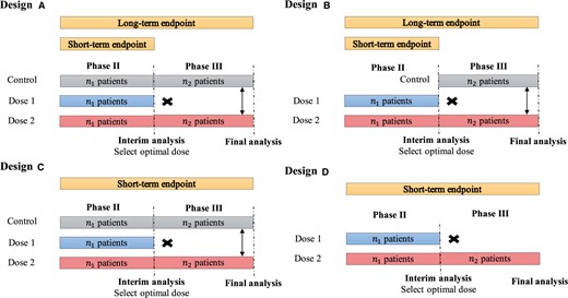
Diagrams of phase II/III designs. Design A: including a concurrent control in both phases, using a short-term binary endpoint (eg, ORR) in phase II to select the optimal dose and using a long-term time-to-event endpoint (eg, PFS or OS) in phase III to evaluate the therapeutic effect of the treatment. In this example, dose 2 is selected as the optimal dose at the end of phase II, and patients are randomly assigned to dose 2 and a concurrent control arm. Design B: a modification of design A, including a control only in phase III. Design C: similar to design A but the short-term endpoint (eg, ORR) is used for phase II dose selection and phase III final analysis. Design D: a simplified version of design C without control in both phases. ORR = objective response rate; OS = overall survival; PFS = progression-free survival.
Depending on whether the concurrent control is included and the type of endpoints used in phase II /III, we distinguish 4 forms of (inferential) phase II/III dose-optimization designs that are suitable for different clinical settings (see Figure 1). Design A includes a concurrent control in both phases and employs a short-term binary endpoint (eg, ORR) in phase II to select the optimal dose. Phase III utilizes a long-term time-to-event endpoint (eg, PFS or OS) to evaluate the treatment’s therapeutic effect. The use of a short-term endpoint in phase II allows for a timely selection of the optimal dose to proceed to phase III. One notable characteristic of design A is that patients in phase II are followed continuously to evaluate their long-term time-to-event endpoint (eg, PFS or OS); and data from both phases are combined for the final analysis of PFS or OS. Thus, phase II/III designs are more efficient and can potentially reduce the sample size. Although not depicted in the diagram, if appropriate, phase III may include additional interim futility and/or superiority analyses similar to the standard group sequential design (21-23). An example of design A is the double-blind randomized phase III study that compared the efficacy of cediranib with bevacizumab for the treatment of advanced metastatic colorectal cancer (24).
Design B is a modification of design A that includes a control only in phase III (see design B), resulting in a further reduction in sample size. However, the drawback of design B is that because of the lack of a concurrent control in phase II, it can be challenging to combine data from phase II/III to obtain an unbiased estimate of the treatment effect when there is a drift in the patient population between 2 phases. Despite this limitation, design B is still a reasonable choice when a drift is unlikely. Design B has been used in several clinical trials, such as a randomized multicenter trial of SM-88 in patients with metastatic pancreatic cancer (25) and a randomized phase II/III study evaluating AL102 in desmoid tumors (26).
Design C is similar to design A, but the short-term endpoint (eg, ORR) is used for dose selection and final analysis. This design is suitable when demonstrating an effect on the long-term endpoint (eg, survival or morbidity) requires lengthy and sometimes large trials because of the disease’s duration, and the short-term endpoint is reasonably predictive of clinical benefit on the long-term endpoint (27-29). An example of design C is the phase II/III study comparing intravenous tenecteplase to standard-dose intravenous alteplase for treating patients with acute ischemic stroke (30).
Design D is a simplified version of design C, which does not include a control. It is suitable for situations where there is an urgent unmet medical need (eg, a refractory or resistant patient population) and/or the tumor under treatment is rare. Designs C and D are especially useful for drug development that targets accelerated approval from the FDA, which is often based on a short-term surrogate or intermediate clinical endpoint such as ORR. However, like design B, a limitation of design D is the lack of concurrent controls, which may lead to a biased estimate of the treatment effect when there is a drift in the patient population.
In designs A-D, the 2 crucial decision points are the selection of the optimal dose at the end of phase II and the determination of the treatment effectiveness at the end of phase III. The following section will describe design considerations related to these decision points.
Selection of optimal dose
At the end of phase II, the selection of the optimal dose with the most desirable benefit-risk trade-off is crucial for further efficacy and safety evaluation in phase III. The metrics used to quantify the benefit-risk trade-off and guide dose selection may vary depending on the trial setting. For ease of exposition, we focus on a toxicity endpoint and an efficacy endpoint, noting all available data (eg, tolerability and PK-PD) should also be taken into account. Given a dose d, let and denote its efficacy rate and toxicity rate, respectively. A straightforward measure for the benefit-risk trade-off (or desirability) of d is
where is a prespecified weight. This efficacy-toxicity probability-based desirability measure says that for a dose with a given efficacy and toxicity profile, a dose with 10% better efficacy and (10/)% increased toxicity is equivalently desirable. A larger value of favors selecting a dose with lower toxicity. When , leads to selecting the dose with the highest efficacy rate. Another more flexible approach that contains Equation 1 as a special case is to use utility to quantify the benefit-risk trade-off (31), which may be preferred in practice due to its ease of interpretation. To prevent the selection of toxic and/or futile doses, we require that the optimal dose must demonstrate a lower toxicity rate and a higher efficacy rate than predetermined limits based on Bayesian posterior probability criteria. If none of the doses satisfy the criteria, the trial should stop early after phase II (see Supplementary Material A, available online).
Final analysis of significance
The other key decision point occurs at the end of phase III when evaluating if the treatment effect of the selected optimal dose is statistically significant compared with the concurrent or historical control. Directly pooling phase II/III data and applying a standard testing method (eg, log-rank or χ2 test) is problematic. This is because the dose evaluated in phase III is selected as the dose that has demonstrated the promising treatment effect, resulting in intrinsically biased phase II/III combined data toward a positive treatment effect and thus inflating the type I error. To address this issue, various statistical methods have been proposed to control the family-wise error rate (FWER) [see Stallard and Todd (13) and Kunz et al. (14)]. In our simulation, we used the combination test with the closed testing procedure (15,16) to control FWER. The technical details of the closed testing procedure are provided in Supplementary Material B and Supplementary Figure 1 (available online).
Evaluation of phase II/III dose-optimization designs
The standard definition of power, which is the probability of rejecting the null hypothesis that the treatment is not more efficacious than the control when the treatment is truly effective, is not sufficient to characterize the operating characteristics of phase II/III dose-optimization designs. This is because power does not consider the dose selection process, and we may choose a wrong dose and reject the null hypothesis. Therefore, we introduce the generalized power, which accounts for both selecting in phase II and testing in phase III. It is defined as the probability of correctly selecting the optimal dose and also rejecting the null hypothesis, assuming the treatment is truly effective. In addition to the generalized power, it is also important to assess the performance of phase II dose selection. This can be quantified by the percentage of correction selection (PCS) of the optimal dose at the end of phase II.
Simulation studies
We conducted simulations to assess the operating characteristics of designs A-D. We considered 3 scenarios when 2 doses were evaluated in phase II, and 4 scenarios when 3 doses were evaluated. Table 1 and Supplementary Table 1 (available online) show the scenarios for the null ORR of 0.2 vs a target ORR of 0.4 and 0.1 vs 0.3, respectively. We used the benefit-risk trade-off in Equation 1 with to select the optimal dose. The Bayesian safety and efficacy criteria were used to prevent the selection of toxic and/or futile doses. For phase III, the null and target hazard ratios were 1 and 0.64, respectively. Sample sizes for phase II/III ( and per arm, respectively) were chosen to achieve 80% generalized power. For example, when 2 doses were evaluated and the null and target ORRs were 0.2 and 0.4, respectively, ( (50, 100) for design A, (50, 115) for design B, (50, 80) for design C, and (45, 30) for design D. When 3 doses are evaluated, ( (80, 100) for design A, (80, 110) for design B, (90, 60) for design C, and (80, 20) for design D. We also assessed the impact of population drift on designs B and D and evaluated the influence of different choices of and on design performance by varying the ratio of and with a fixed total sample size . Further information on the data generation methods and simulation settings can be found in Supplementary Materials C and D (available online).
Efficacy rate, toxicity rate, and hazard ratio for 2-dose and 3-dose scenariosa
| Scenario | 2-dose | 3-dose | ||||||||||||||||
|---|---|---|---|---|---|---|---|---|---|---|---|---|---|---|---|---|---|---|
| 0 | 1 | 2 | 0 | 1 | 2 | 3 | ||||||||||||
| Dose | 1 | 2 | 1 | 2 | 1 | 2 | 1 | 2 | 3 | 1 | 2 | 3 | 1 | 2 | 3 | 1 | 2 | 3 |
| Efficacy rate | 0.20 | 0.20 | 0.40 | 0.40 | 0.22 | 0.40 | 0.20 | 0.20 | 0.20 | 0.39 | 0.40 | 0.41 | 0.20 | 0.40 | 0.40 | 0.20 | 0.26 | 0.40 |
| Toxicity rate | 0.30 | 0.30 | 0.13 | 0.29 | 0.13 | 0.26 | 0.30 | 0.30 | 0.30 | 0.11 | 0.28 | 0.30 | 0.11 | 0.18 | 0.30 | 0.24 | 0.25 | 0.30 |
| Hazard ratio | 1.00 | 1.00 | 0.64 | 0.64 | 0.97 | 0.64 | 1.00 | 1.00 | 1.00 | 0.64 | 0.63 | 0.62 | 0.95 | 0.64 | 0.62 | 0.96 | 0.79 | 0.64 |
Scenario 0 represents a null case where all doses are ineffective and thus has no optimal dose. In 2-dose scenarios, scenarios 1 and 2 represent the optimal doses are doses 1 and 2, respectively; and in 3-dose scenarios, scenarios 1-3 represent the optimal doses are doses 1-3, respectively. The optimal dose is indicated in boldface.
To demonstrate the potential benefit of phase II/III designs in reducing the required sample size, we compared designs A-D with their noninferential or operational counterparts (denoted as NI), which disregard phase II data, and the counterparts with only the highest dose evaluated in phase II (denoted as HD). Supplementary Material D (available online) displays and of NIs with generalized power matched to designs A-D. For HDs, remains the same as that of designs A-D, whereas is calibrated by achieving 80% power in phase III. We conducted 10 000 simulations for each scenario and calculated the FWER, PCS, generalized power, average total sample size, and toxicity rate in treatment arms.
Results
In null scenarios with all doses being ineffective (scenario 0), designs A-D effectively control the FWERs under 5% (see Supplementary Figure 2, available online). The PCS and generalized power are depicted in Figures 2, A and B, respectively. Designs A-D yield PCS above 80% (Figure 2, A) and generalized power around 80% (Figure 2, B) across scenarios. Figure 2, C, displays the average sample sizes of designs A-D, which are considerably smaller than those of NIs. Depending on the design and scenario, the sample size savings range from 16.6% to 27.3%, with a mean savings of 22.1%. For example, for the 2-dose setting, design A saves 16.7% and 16.6% sample size for scenarios 1 and 2, whereas design D saves 25.0% and 24.8%. It appears that design B provides greater sample size savings than design A, and design C provides more savings than design D. For instance, in 2-dose scenario 1, design B saves 4.8% more sample size than design A, and in 3-dose scenario 2, design C saves 8.5% more sample size than design D. Figure 2, D, shows the toxicity rates of designs A-D, which are lower than those of HDs, especially when the lower dose is optimal. For example, in 2-dose scenario 1 and 3-dose scenario 2, design A has 0.11 and 0.09 lower, design B has 0.11 and 0.1 lower, design C has 0.11 and 0.08 lower, and design D has 0.09 and 0.08 lower toxicity rates than HDs. This demonstrates the benefit of dose optimization. The results are similar under different null and target ORRs (0.1 vs 0.3); see Supplementary Figure 3 and Supplementary Material E (available online).
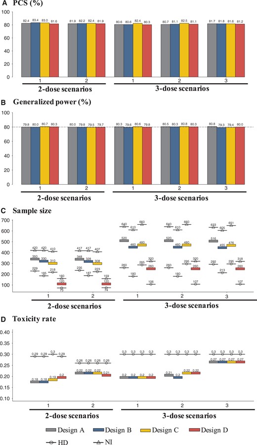
A) The percentage of correct selection (PCS) of the optimal dose, (B) generalized power (%), (C) the average sample size, and (D) the toxicity rate of designs A-D, with the null and target ORRs of 0.2 and 0.4, respectively, and the target hazard ratio of 0.64. In panels (C) and (D), NI represents noninferential or operational counterparts of designs A-D, which disregard phase II data, and HD represents the counterparts with only the highest dose evaluated in phase II. ORR = objective response rate; PCS = percentage of correction selection.
As anticipated, design B requires a substantially smaller sample size than design A because of the absence of a concurrent control in phase II. For instance, in 3-dose scenario 3, the sample size of design B is 60.4 less than that of design A. Similarly, design D requires a smaller sample size than design C. However, a limitation of designs B and D is that they lack a concurrent control in phase II or both phases, which may result in a biased estimate of the treatment effect in the presence of patient population drift. Supplementary Figure 4 (available online) displays the FWER and generalized power of designs B and D when there is a positive or negative drift. Positive drift leads to FWER inflation from 5% to as much as 13%, whereas negative drift reduces power from 80% to 70% in some cases.
We also studied how the phase II sample size (ie, ) affects the performance of the designs while keeping the total sample size fixed. The results for design C under 2-dose scenario 1 and 3-dose scenario 2 are presented in Figure 3, with similar results observed for other scenarios (see Supplementary Figure 5, available online). We found that the generalized power initially increases with and then starts to decrease after reaches a certain value. For example, in 3-dose scenario 2, the generalized power increases up to approximately 80% when , nearly plateaus from to , and then begins to decrease. This highlights the importance of carefully allocating sample sizes between the 2 stages when conducting phase II/III trials to achieve maximum efficiency.
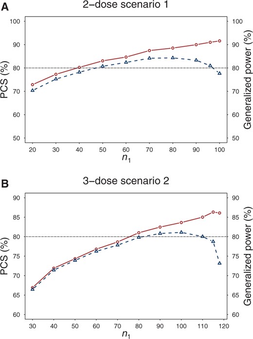
The percentage of correct selection (PCS) (solid lines) of the optimal dose and generalized power (dashed lines) of design C under different phase II sample size per arm in a 2-dose scenario 1 and 3-dose scenario 2. The total sample size is fixed. PCS = percentage of correction selection.
Furthermore, we evaluated the performance of designs A-D using the utility method to quantify the benefit-risk trade-off (detailed in Supplementary Material A1, available online). The results (see Supplementary Figure 6, available online) were generally similar to the findings above. Designs A-D had similar PCS and generalized power but substantially lower average sample sizes than NIs, as well as lower toxicity rates than HDs.
Discussion
We have systematically investigated the operating characteristics of phase II/III designs for dose optimization. Our simulation results demonstrate that these designs can yield comparable power and type I error control to conventional methods while requiring a substantially smaller sample size. This makes them a valuable option for addressing the challenges of limited accrual and tight timelines in oncology dose optimization trials. Depending on the specific trial objectives and endpoints, one of designs A-D can be selected. Designs A and C are recommended in the presence of patient population drift, and designs B and D are suitable when such drift is unlikely, because of their smaller sample sizes. Furthermore, other types of phase II/III designs, such as those involving different survival endpoints (eg, PFS in phase II and OS in phase III), may also be considered.
Phase II/III designs for dose-optimization face logistical and operational challenges. Early meetings between sponsors and regulatory agencies are important to clarify expectations and improve efficiency. Unblinded data access at the end of phase II is necessary for dose selection but requires careful management to maintain trial integrity. A data monitoring committee or independent adaptation body should make interim dose selection decisions, with safeguards in place to ensure confidentiality and adherence to operating procedures. Prespecification of trial details and data access plan, particularly FWER control, is crucial for trial integrity.
Our simulation assumes that the short-term endpoints (eg, ORR and toxicity) are concordant with long-term endpoints (eg, OS and tolerability), such that the optimal dose selected at the end of phase II is still optimal in terms of phase III endpoints. One important issue we did not investigate is the impact of discordance between short-term and long-term endpoints on the operating characteristics of phase II/III designs. If ORR and OS are discordant, deriving a useful desirability ranking for dose selection would be challenging. This issue, however, is not specific to phase II/III trials and also occurs in the conventional separated phase II/III trials. One way to alleviate this issue is to conduct long-term follow-up in phase II, before starting phase III, and make decisions based on long-term endpoints. This approach in principle can also be applied to phase II/III trials by pausing the accrual at the end of phase II to collect long-term endpoints for dose selection, although it may not be practical in some trials. This would maintain the sample size saving observed for phase II/III designs because long-term endpoint data collected in both phases can still be combined for more efficient inference. Some work has been done on this issue (14,19), but more research is needed. One possible approach is sequential adaptive phase II/III designs, where dose arms are continuously updated based on accumulative short-term and long-term data.
Other design strategies are available for dose optimization [eg, phase I/II designs (32,33)] that integrate phase I and II trials. Examples include the EffTox design (34) and BOIN12 design (31). As dose optimization and selection have been completed before onset of the confirmative trial, a phase II/III design approach simplifies the implementation of confirmation trials, which may be appealing in some cases.
Data availability
All data and simulation study in this paper were generated by the computer code, which is openly available upon request for research use.
Author contributions
Liyun Jiang, PhD (Conceptualization; Formal analysis; Investigation; Methodology; Software; Validation; Visualization; Writing—original draft; Writing—review & editing) and Ying Yuan, PhD (Conceptualization; Formal analysis; Investigation; Methodology; Software; Supervision; Writing—original draft; Writing—review & editing).
Funding
This research was supported by Award Number P50CA221707, P50CA127001 and CA016672 from the National Cancer Institute.
Conflicts of interest
None.
Acknowledgements
We acknowledge the National Cancer Institute for supporting YY in the analysis, simulation, interpretation of the results, and writing of the manuscript. No prior presentation.
References
A study of AL102 in patients with progressing desmoid tumors (RINGSIDE). ClinicalTrials.gov identifier: NCT04871282. Updated June 10, 2022. https://clinicaltrials.gov/ct2/show/NCT04871282.

