The Welfare-Enhancing Role of Parental Leave Mandates

Abstract

A major factor that contributes to persistent gender variation in labor market outcomes is women’s traditional role in the household. Child-related absences from work imply that women accumulate less job experience, are more prone to career discontinuities and, hence, suffer a motherhood penalty. We highlight how the gender-driven career/family segmentation of the labor market may create a normative justification for parental leave rules as a means to enhance efficiency in the labor market and alleviate the gender wage gap. (JEL D82, H21, J31, J83)

1. Introduction

There is a voluminous body of evidence documenting gender variation in labor market outcomes, including differences in employment rates, working hours, earnings, and job composition (in terms of sector, occupation type, and scope). A recent survey by Olivetti and Petrongolo (2016) reviews the existing literature and points out that despite a post-war convergence process, reflecting a host of supply side factors, including medical advances (availability of birth control), human capital investment (access to higher education), and family-friendly policies (provision of affordable child care services and generous parental leave arrangements), substantial gender differences in pay and employment levels still remain.

A major factor that contributes to persistent gender gaps in labor market performance is parenthood. Women, who traditionally take the lion’s share of responsibility for the caring of children, tend to have less job experience, greater career discontinuity, and shorter work hours, resulting in worse labor market outcomes.¹ Indeed, there is now a large and growing empirical literature documenting the wage penalty associated with motherhood. For instance, for women in the United States, the average wage penalty associated with an additional child is around 5%, and persists even when workplace factors and education are controlled for (Waldfogel 1997; Budig and England 2001).

Goldin (2014) argues that workplace flexibility is a key factor in explaining gender wage differences. She discusses multiple dimensions of job flexibility, including the number of hours at work, the precise (particular) times worked, and the predictability and ability to set the work schedule. She further argues that such flexibility is costly for the firm, alluding to mechanisms such as the limited ability of workers with discontinuous work schedules to interact with co-workers and clients, which may hamper the transmission of vital job-related information. This implies that flexible jobs pay less, and workers are faced with a fundamental trade-off between flexibility and compensation. For instance, high skill mothers may compromise by selecting into part-time, low-level, flexible jobs, rather than pursuing a professional challenging career, as documented by Blau and Kahn (2013).

The degree of workplace flexibility granted to workers reflects institutional arrangements in the labor market and prevailing norms but is, to a large extent, shaped by government policy. A notable example is parental leave rules. The latter, taking a broad perspective, refer to the legal framework regulating the extent to which firms must grant their employees child-related absences from work. The most basic form of parental leave refers to the time parents are permitted to take off work in order to take care of a newborn child, but in many countries parental leave extends beyond the care of infants, to encompass additional aspects of workplace flexibility, such as allowing parents to take time off work to take care of an older child, or to take care of a sick child.

There are large differences across countries in terms of the generosity of parental leave, such as the duration of leave, the level of benefits, job protection features, and eligibility (for a comprehensive recent survey, see Rossin-Slater 2017). The United States is a country with one of the least generous systems where the flexibility of labor contracts with respect to child-related absences is largely a decision made by employers. The federal Family and Medical Leave Act, which ensures that parents can leave their jobs for 12 weeks and then come back, does not apply to small firms with less than 50 employees. Parental leave in Europe, and especially in the Nordic countries, is significantly more generous. According to the Parental Leave Directive of the European Union (2010/18/EU) parental leave allowances in EU countries must be at least 4 months for each parent.²

In this paper, we explore a novel normative justification for parental leave rules in the presence of a fundamental gender-driven career/family (compensation/flexibility) conflict faced by workers in the labor market. We consider a benchmark framework where firms are unable to offer distinct contracts to workers differing in their career/family orientation due to asymmetric information, or, by virtue of anti-discrimination legislation that prevents them from doing so. We show that in such a setting, a distortion arises taking the form of an underprovision of workplace flexibility. We then demonstrate that the government can make use of parental leave mandates, as a means to regulate the extent of workplace flexibility, thereby mitigating the distortion and also promoting redistributive goals via reducing the extent of gender pay gaps.

The paper is organized as follows. In Section 2, we discuss the related literature and in Section 3, we outline our model and present the efficient symmetric information laissez-faire allocation. We then present our benchmark setting with asymmetric information and demonstrate the distortion associated with an underprovision of workplace flexibility. In Section 4, we show how introducing parental leave mandates can possibly mitigate this distortion, resulting in a Pareto-improvement. In Section 5, we examine the socially desirable parental leave policy and discuss the implications for gender equality. Section 6 presents some extensions of our analysis and, finally, Section 7 offers concluding remarks.

2. Related Literature

Since the seminal contribution of Rothschild and Stiglitz (1976), minimum coverages have been identified as means to achieve efficiency in insurance contexts where the focus is on asymmetric information regarding heterogeneity in risk types. A general discussion of the social desirability of mandates is provided by Summers (1989) who emphasizes the role played by mandates in correcting for externalities, and the connection between mandates and public provision of private/public goods. In the context of annuities, Eckstein et al. (1985) show that a minimum mandated coverage and the ability to buy insurance beyond the minimum can yield Pareto improvements. In the context of health insurance, mandates have been analyzed by Neudeck and Podczeck (1996), Encinosa (2001), Finkelstein (2004), and McFadden et al. (2015), using a variety of equilibrium concepts. Hackmann et al. (2015) is an empirical application, developing a model of the individual health insurance market in the United States, analyzing the impact of an individual mandate on adverse selection, computing the associated welfare gains. Mandates have also been discussed in the sick-leave literature. For example, Pichler and Ziebarth (2017) discuss how mandated paid sick leave can be desirable on efficiency grounds in a setting where firms have imperfect information about the contagiousness of sick workers present in the workplace.³

Our paper differs from the above literature in several ways. We study an adverse selection problem deriving from differences in preferences (career versus family orientation) which in conjunction with anti-discrimination legislation induce firms to behave as if they operate under asymmetric information. We thus take insights from the insurance literature and apply them in a different context where we study the role of parental leave mandates. We shed light on positive aspects (such as motherhood penalties and gender wage gaps arising in our benchmark equilibrium), the efficiency aspect of a parental leave mandate as a means to inject missing flexibility in the labor market, as well as normative aspects of an optimal parental leave system that mitigates gender wage gaps. We consider novel aspects such as the combination of mandates and taxation and the possibility to attain a pooling equilibrium through an appropriately chosen parental leave mandate, which has implications for gender equality in the labor market.

By providing a normative justification for parental leave mandates, our paper also relates to a small and recent theoretical literature on the effects of this particular form of government intervention. This includes Barigozzi et al. (2017) and Del Rey et al. (2017). The former contribution emphasizes the interaction between parental leave policy, externalities generated through endogenous social norms concerning child care activities, and career choices; the latter investigates the effects of parental leave on unemployment and wages in a search and matching model of the labor market.

Two other related papers are Thomas (2018) and Bronson (2015). The former analyzes the welfare effects of government-mandated maternity leave policies from the perspective that they can change employer’s expectations of women’s future labor supply, and therefore, the incentives for employers to invest in their workers.⁴ The latter constructs and estimates a dynamic structural model of marriage, education choices, and life-time labor supply where the ‘work/family’ flexibility of jobs and educational tracks plays an important role.⁵

Finally, and more broadly, our paper also relates to a recent strand in the literature that examines the optimal design of public policy in environments with two layers of asymmetric information, between the government and the agents and between private actors in the market (see Stantcheva 2014; Bastani et al. 2015; Cremer and Roeder 2017).

3. Model

We consider a simple labor market with an identical number of equally skilled female and male workers. Each worker is endowed with a fixed amount of time (normalized to unity) that is allocated between work time and time spent with his/her children (parental leave). Workers differ in their career/family orientation, which is reflected in the propensity to take parental leave. We simplify by assuming that workers can be either career-oriented (with a low propensity to take a leave) or family-oriented (with a high propensity to take a leave). We refer to career-oriented workers as type 1 and to family-oriented workers as type 2, and denote their respective fractions in the population by $γ^{i}, i = 1, 2$ where the total population size is normalized to unity, without loss of generality. We let θ^j, $j = m, f,$ denote the fraction of family-oriented workers among men and women, respectively. We assume realistically that $θ^{f} > θ^{m}$ ⁠, reflecting that women exhibit, on average, a stronger family orientation. This implies that $γ^{2} = \frac{θ^{f} + θ^{m}}{2}$ and $γ^{1} = 1 - γ^{2}$ ⁠.

The utility function of a type i worker is given by

U^{i} (c^{i}, α^{i}) = c^{i} + π^{i} v (α^{i}),

(1)

where c denotes total consumption (over the unit endowment of time), α denotes the duration of parental leave, and πⁱ denotes the propensity/likelihood that a type i worker will take parental leave (where

π^{2} > π^{1}

⁠). One possible interpretation of this propensity is the expected number of children. The function v is assumed to be strictly increasing and strictly concave.

For tractability, we simplify by invoking a quasi-linear specification and by assuming that the propensity to take parental leave, πⁱ, is exogenous. We relax both these assumptions in Section 6.3, where we show that these assumptions do not change the qualitative nature of our results.⁶

We assume that the labor market is perfectly competitive. Firms do not observe the family orientation of workers or, alternatively, firms are prevented by some form of anti-discrimination legislation, from tagging workers based on observable characteristics correlated with family orientation, such as gender, age, the number and age of children, or marital status.⁷ Thus, firms instead rely on screening employment contracts. A typical labor contract offers the worker a given amount of (monetary) compensation y (which is also equal to the workers’ consumption c in the absences of taxes and transfers), and a given duration of parental leave, α. The latter captures the extent of workplace flexibility, which essentially is an option to take a pre-specified amount of time off work, should family circumstances demand it.

Free entry implies that firms break even in expectation. Thus, a firm offering a contract

(y^{i}, α^{i})

to a type i worker must satisfy

y^{i} = 1 - π^{i} α^{i},

(2)

where

π^{i} α^{i}

is the total expected time worker i will be away from work and where we have normalized the productivity of the worker per unit of time to 1. The greater the extent of workplace flexibility offered to a worker, the lower is the compensation that he/she receives. Our setup thus captures in a simplistic form a fundamental tension between compensation and flexibility.

The variation in career/family orientation across workers affects both the demand and supply of workplace flexibility. From the workers’ perspective, a stronger family orientation is reflected in a higher willingness to pay for additional flexibility (extended parental leave). From the firms’ perspective, a family-oriented worker, being more likely to be absent from work, is (in expected terms) less productive than an equally skilled career-oriented counterpart.

3.1 Symmetric Information Equilibrium

The symmetric information equilibrium reflects a situation where firms are able to observe or infer the family orientation of workers, and, at the same time, are not prevented by law from discriminating between workers. Thus, in the symmetric information equilibrium, the firm can offer distinct contracts to workers of type 1 and type 2. The symmetric information contracts maximize the utility in (1) subject to the budget constraint (2) resulting in an efficient labor market equilibrium satisfying the familiar tangency condition:

\frac{1}{π^{i} v' (α^{i})} = \frac{1}{π^{i}} \Leftrightarrow 1 = v' (α^{i}) .

(3)

The optimal contract, for each type of worker (i = 1, 2), is given by the solution to a system of two equations: the zero profit condition (budget constraint) in Equation (2) and the tangency condition in Equation (3). The optimum for type i = 1, 2 is illustrated graphically in Figure 1 (where ZP1 and ZP2 refer to the zero profit lines). Point A represents the contract offered to type 2 workers and point B represents the contract offered to type 1 workers. Note that because of the heterogeneity in π, agents have differently sloped budget- and indifference curves in the

(c, α)

space.

Figure 1.

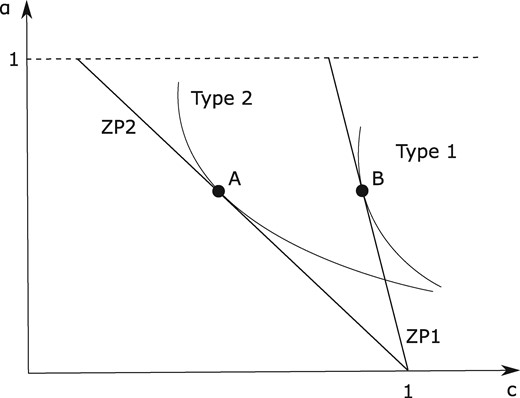
Efficient equilibrium. Point A illustrates the efficient contract offered to type 2 workers and point B represents the efficient contract offered to type 1 workers.

Open in new tab Download slide

Straightforward full differentiation of the system of equations given by Equations (2) and (3) with respect to π, noting that c = y in the absence of any taxes or transfers, yields the following comparative statics: $c^{1} > c^{2}, α^{1} = α^{2}$ and $π^{2} α^{2} > π^{1} α^{1}$ ⁠. The two contracts offer the same degree of flexibility $(α^{1} = α^{2})$ but family-oriented workers suffer a wage penalty as they have a higher expected workplace absence (⁠ $π^{2} α^{2} > π^{1} α^{1}$ ⁠).

The fact that in the efficient symmetric information allocation, both types of workers are offered the same parental leave is driven by our simplifying assumptions which are made for tractability.

First, we have assumed that both types of workers derive the same utility from each parental leave spell. It is, however, plausible that family-oriented workers would assign a higher value to time spent with their children. Second, we have assumed that the only difference between the two career paths is in the total expected time that workers spend on the job, which is reflected in their output and remuneration. In reality, not only total hours, but also the particular hours matter (i.e., being available for clients and peers at the workplace), suggesting that workers holding family friendly (flexible) jobs are less productive per unit of time relative to equally skilled workers who hold career-oriented jobs (see Goldin [2014] and our discussion in Section 1).⁸ These assumptions are relaxed in two extensions of our model in Section 6 where family-oriented workers, in the efficient symmetric information equilibrium, are offered a longer parental leave than their equally skilled career-oriented counterparts (and, accordingly, suffer an even larger wage penalty).

3.2 Benchmark Equilibrium with Asymmetric Information

We now proceed to consider the realistic case where firms either can not observe or infer the family orientation of workers, or, are prevented from offering distinct contracts to type 1 and type 2 workers, due to some form of anti-discrimination legislation. This will serve as our benchmark equilibrium.

When firms are not allowed to discriminate directly, they do it indirectly, by offering workers the choice to self-select into two career paths: (i) family-oriented jobs that offer greater flexibility with respect to child-related absences from work but a lower compensation and (ii) career-oriented jobs that demand longer work hours but offer a higher compensation.

The labor market equilibrium is defined by a set of labor contracts satisfying two properties: (i) firms make non-negative profits on each contract and (ii) there is no other potential contract that would yield non-negative profits if offered (in addition to the equilibrium set of contracts).⁹Figure 2 illustrates the separating equilibrium, along with the symmetric information equilibrium. Notice that a pooling equilibrium in which both types of workers are offered an identical bundle cannot exist due to ‘cream-skimming’. Firms can always break a pooling contract, and derive positive profits, by offering a bundle (with lower flexibility and higher compensation), which would attract career-oriented workers only.¹⁰

Figure 2.

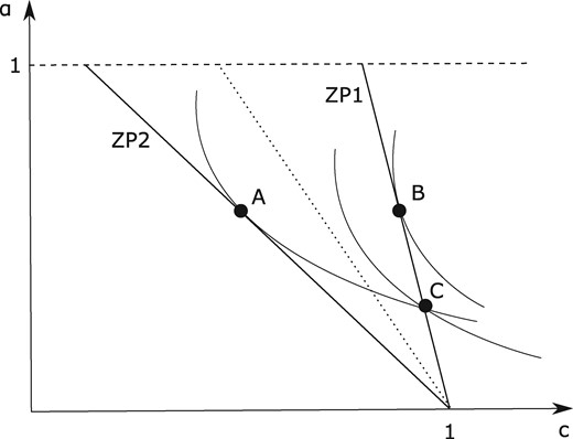
Benchmark equilibrium. Type 2 workers are offered their efficient contract A and type 1 workers contract C, rather than the efficient contract B.

Open in new tab Download slide

Notice that when the efficient contracts from Section 3.1 (points A and B in the figure) are available to both types of workers, each of them will prefer the contract intended for type 1 workers (point B in the figure). Hence, the separating allocation associated with the symmetric information case cannot form an equilibrium, since it is not incentive compatible.

The separating equilibrium will maintain the efficient contract depicted by point A, which would still be offered to type 2 workers in the presence of asymmetric information. However, type 1 workers must be offered the contract depicted by point C in the figure, which lies on the intersection of the indifference curve of type 2 going through point A and the zero profit curve, associated with type 1 workers. Rather than maximizing the utility of type 1 worker subject to the zero profit condition (as happens in the efficient case), the new contract, C, maximizes the utility of type 1 subject to both the zero profit condition and the binding incentive constraint of type 2 workers, ensuring that type 2 workers would be indifferent between choosing point A and mimicking type 1 by choosing point C. The latter binding incentive constraint is the source of inefficiency. Notice that the indifference curve of type 1 intersects (rather than being tangent to) the zero profit curve associated with type 1 workers. Thus, the resulting allocation implies that type 1 workers will obtain less parental leave, and correspondingly obtain a higher compensation, than under the symmetric information equilibrium, yielding them a lower level of utility.¹¹

For later purposes, we accompany the informal graphical illustration of this benchmark equilibrium with a formal definition:

Definition 1.

(Benchmark Equilibrium). The benchmark labor market equilibrium is given by the bundles $(c^{1 *}, α^{1 *})$ and $(c^{2 *}, α^{2 *})$ associated, correspondingly, with type 1 and type 2 workers, where $c^{1 *}, α^{1 *}, c^{2 *}, α^{2 *}$ solve the two zero profit conditions $c^{i *} = 1 - π^{i} α^{i *}, i = 1, 2$ ⁠, the condition $1 = v' (α^{2 *})$ (the requirement that the bundle of type 2 is undistorted) and the condition $c^{2 *} + π^{2} v (α^{2 *}) = c^{1 *} + π^{2} v (α^{1 *})$ (the requirement that type 2 is indifferent between choosing her bundle and mimicking by choosing the bundle of type 1).

In order for the separating equilibrium to exist, we need to rule out the possibility for a firm to offer a labor contract (in addition to the equilibrium set of contracts) that would yield non-negative profits. To ensure existence of a separating equilibrium, we henceforth make the following assumption:

Assumption 1.

max_{α} 1 - α \sum γ^{i} π^{i} + π^{1} v (α) < c^{1 *} + π^{1} v (α^{1 *}),

where

(c^{1 *}, α^{1 *})

denotes the type 1 bundle associated with the separating benchmark equilibrium.

Assumption 1 implies that type 1 workers strictly prefer their separating equilibrium contract to any pooling contract that yields zero profits. In Figure 2, this assumption is satisfied.

3.3 The Gender Wage Gap in the Benchmark Equilibrium

While the key focus of this paper is normative issues, there is an important positive aspect of our benchmark equilibrium that we would like to point out, and which relates to the recent debate about the persistent gender wage gaps mentioned in Section 1.

In the benchmark equilibrium, family-oriented workers earn less than career-oriented workers of the same skill level. As we have assumed, realistically, that there is a higher fraction of family-oriented workers among women (i.e., $θ^{f} > θ^{m}$ ⁠), it follows that in the benchmark equilibrium, on average, female workers suffer a wage penalty relative to their equally skilled male counterparts. Notice that this is the case even in the symmetric information efficient equilibrium, but the inability of firms to perfectly tag workers further exacerbates the gender pay gap relative to the symmetric information equilibrium. Ironically, to the extent that the inability of implementing the symmetric information equilibrium is related to anti-discrimination legislation preventing firms from engaging in tagging, one potential implication would be that anti-discrimination legislation, in and of itself, is counter-productive in promoting equal pay for men and women in the labor market.

Our model is consistent with empirical evidence alluding to the importance of sorting across career tracks as an explanation for gender differences in labor market outcomes, where female workers to a larger extent sort into family-friendly tracks.

4. The Efficiency-Enhancing Role of Parental Leave

We now focus on the consequences of setting a lower bound on the duration of parental leave at a level that is slightly above the amount prescribed, at the benchmark equilibrium, by the contract intended for career-oriented workers. Formally, a binding mandatory parental leave rule, denoted by $\bar{α}$ ⁠, implies that in equilibrium the following condition has to hold: $α^{i} \geq \bar{α}; i = 1, 2$ ⁠, where $\bar{α} > α^{1 *}$ ⁠. As it turns out, the government can use a parental leave mandate to inject the ‘missing’ flexibility into the labor market, thereby correcting the market failure present in the benchmark equilibrium.¹² In Section 4.1, we characterize the labor market equilibrium in the presence of a parental leave mandate. We start by an informal (graphical) description and then provide a formal definition. In Section 4.2, we turn to address the normative question regarding the desirability of parental leave mandates on efficiency grounds.

4.1 Equilibrium in the Presence of a Parental Leave Mandate

We recall two properties of the benchmark equilibrium: (i) the incentive constraint of type 2 agents is binding (in order to maintain incentive-compatibility type 1 workers have to be offered the point C rather than the efficient contract B) and (ii) the contract offered to type 2 agents is efficient. These two properties of the benchmark equilibrium carry over to the separating equilibrium with parental leave.

In Figure 3, we present the benchmark equilibrium, illustrated as points A and C in the figure, along with a binding parental leave rule $α = \bar{α}$ ⁠. The parental leave rule is chosen to be binding, so that it renders the point C infeasible but does not constrain the efficient contract offered to type 2 (point A). The fundamental difference between the benchmark allocation and the one arising in the presence of a parental leave rule is that in the former, the allocation of a type 1 worker is given by the intersection of the indifference curve of type 2 worker (going through his/her equilibrium allocation) and the zero profit line associated with firms hiring type 1 workers (point C in Figure 3), whereas in the latter, it is given by the intersection of the indifference curve of type 2 (going through his/her equilibrium allocation) and the parental leave rule line $α = \bar{α}$ ⁠. This is illustrated by point D in Figure 3.

Figure 3.

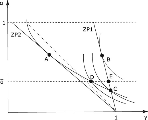
Equilibrium with parental leave. The contract depicted by point C in the figure is no longer feasible due to the presence of the parental leave rule.

Open in new tab Download slide

Notice that since the parental leave rule is binding by assumption, the equilibrium contract offered to type 1 workers gives rise to positive profits for firms hiring them. This is illustrated in Figure 3 by virtue of the fact that point D lies below the zero profit line ZP1. The reason firms hiring type 1 workers can derive positive profits in equilibrium is the binding parental leave. The latter prevents a new firm from entering the market and offering a contract with a slightly lower value of α in exchange for a slightly higher compensation, which would attract type 1 workers only, and still maintain non-negative profits. We assume that the government taxes these profits and rebate the tax revenues back to agents in a lump-sum manner. An illustration of an equilibrium with both the parental leave rule and the lump-sum transfer in place can be found in Figure 4. Due to quasi-linearity, the lump-sum transfer is reflected in an equal shift of points A and D to the right. The figure illustrates a Pareto-improvement relative to the benchmark allocation, but this does not necessarily need to be the case. We explore this in the next subsection.

Figure 4.

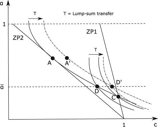
Illustration of parental leave + lump-sum transfer. The lump-sum transfer implies a shift to the right of points A and D to, for example, points A′ and D′, where the distances AA′ and DD′ are equal. In the example, D′ lies to the right of the indifference curve associated with type 1 in the benchmark equilibrium, hence a strict Pareto improvement is achieved.

Open in new tab Download slide

To formally define the separating equilibrium associated with a parental leave rule, supplemented by pure profits taxation and a (universal) lump-sum transfer, let the profits associated with the contract offered to type 1 workers be denoted by $σ > 0$ ⁠. Total tax revenues associated with this tax on (pure) profits are hence given by $γ^{1} σ > 0$ ⁠. These tax revenues are rebated back to agents in a lump-sum manner. As the population size is normalized to unity, this (universal) lump-sum transfer is also equal to $γ^{1} σ$ ⁠.

Definition 2

The separating equilibrium associated with a parental leave rule, supplemented by pure profits taxation and a (universal) lump-sum transfer, is given by the allocation

(c^{1} (σ^{*}), \bar{α})

and

(c^{2} (σ^{*}), α^{2} (σ^{*}))

where

σ^{*}

is the solution to:

c^{2} (σ) + π^{2} v (α^{2} (σ)) = c^{1} (σ) + π^{2} v (\bar{α}),

(4)

and

{c^{2} (σ), α^{2} (σ)} = \underset{c, α}{argmax} c + π^{2} v (α) s . t . c = 1 - π^{2} α + γ^{1} σ,

(5)

c^{1} (σ) = 1 - π^{1} \bar{α} - σ + γ^{1} σ .

(6)

In the above definition (5) states that type 2 workers receive their efficient contract along the zero-profit line $y^{2} = 1 - π^{2} α^{2}$ ⁠, given the lump-sum transfer $γ^{1} σ$ ⁠, whereas Equation (4) states that the incentive constraint of type 2 workers is binding given the binding parental leave rule and the lump-sum transfer $γ^{1} σ$ ⁠. The consumption of type 1 agents, given by Condition (6), is equal to the output produced by type 1 agents, namely $1 - π^{1} \bar{α}$ (when restricted by the parental leave rule $\bar{α}$ ⁠), minus the pure profits σ, plus the lump-sum transfer $γ^{1} σ$ ⁠.

By virtue of the quasi-linear specification,

α^{2} (σ) = α^{2 *}

(where

α^{2 *}

is the duration of parental leave for a type 2 agent in the benchmark allocation; see Definition 1), hence Condition (4) simplifies to

1 - π^{2} α^{2 *} + γ^{1} σ + π^{2} v (α^{2 *}) = 1 - π^{1} \bar{α} - γ^{2} σ + π^{2} v (\bar{α}) .

(7)

In addition to the simplified condition given in Equation (7), to ensure the existence of an equilibrium associated with the parental leave rule, type 1 workers have to weakly prefer their separating equilibrium allocation to any pooling contract that yields zero profits, given the tax system in place. Formally, the following condition has to hold:

max_{α \geq \bar{α}} 1 - α \sum γ^{i} π^{i} + γ^{1} σ + π^{1} v (α) \leq 1 - π^{1} \bar{α} - γ^{2} σ + π^{1} v (\bar{α}) .

(8)

The left-hand side (LHS) of the inequality in Equation (8) describes the utility associated with the pooling contract, along the zero-profit line, given the lump-sum transfer

γ^{1} σ

⁠. The right-hand side (RHS) is the separating allocation associated with type 1, as characterized above.¹³

One can show that the equilibrium characterized by the equation in Definition 2 is well-defined, namely, by setting a binding parental leave rule, $α^{1 *} < \bar{α} \leq α^{2 *}$ ⁠, there exists a unique value of $σ > 0$ that solves Condition (7). To see this first notice that when the parental leave rule is non-binding, namely $\bar{α} = α^{1 *}$ ⁠, then σ = 0, by construction of the benchmark equilibrium. Further notice that $\frac{\partial}{\partial \bar{α}} [1 - π^{1} \bar{α} + π^{2} v (\bar{α})] > 0$ ⁠, for all $α^{1 *} < \bar{α} \leq α^{2 *}$ ⁠, by virtue of the strict concavity of v and as $v' (α^{2 *}) = 1$ and $π^{2} > π^{1}$ ⁠. Thus, by setting a binding parental leave rule, namely $α^{1 *} < \bar{α} \leq α^{2 *}$ ⁠, the RHS of Condition (7) will be larger than the LHS for σ = 0. Finally notice that by setting $σ = (π^{2} - π^{1}) \bar{α} / γ^{2} > 0$ the LHS of Condition (7) will be larger than the RHS, as $1 - π^{2} α^{2 *} + γ^{1} σ + π^{2} v (α^{2 *}) > 1 - π^{2} \bar{α} + π^{2} v (\bar{α})$ ⁠. Thus, by invoking the intermediate value theorem, continuity implies that there exists some $0 < σ < (π^{2} - π^{1}) \bar{α} / γ^{2}$ that solves Condition (7). As the RHS is strictly decreasing in σ and the LHS is strictly increasing in σ, the solution is unique.

4.2 When Is Parental Leave Efficiency Enhancing?

We now proceed to discuss when the composite reform described in the previous section is Pareto-improving. One may first notice that type 2 workers are unambiguously made better off as they obtain the same labor contract as in the benchmark equilibrium, but in addition receive a lump-sum transfer from the government. Turning next to type 1 workers, there are two conflicting forces at play that determine whether type 1 workers become better off from the reform and, ultimately, whether a Pareto-improvement is attainable. First, introducing a parental leave mandate induces firms hiring type 1 workers to offer a higher level of α. This shifts the type 1 contract in the direction of the first best contract, mitigates the distortion associated with the benchmark allocation, and makes type 1 workers better off. Second, the combination of the confiscatory tax levied on the profits of firms hiring type 1 workers, and the universal lump sum transfer, implies that type 1 workers are effectively paying a tax. This implies that their consumption level is shifted to the left of the zero profit condition (ZP1), making them worse off. Without further restrictions, we only know that the allocation of type 1 workers, after the composite reform, lies along the line $α = \bar{α}$ in Figure 3, between points D and E, which may or may not entail that type 1 workers become better off.

The following proposition provides a necessary and sufficient condition for a Pareto-improvement relative to the benchmark equilibrium.

Proposition 1.

A Pareto improvement exists if-and-only-if

γ^{2} / γ^{1} < \frac{[v' (α^{1 *}) - 1]}{v' (α^{1 *}) (π^{2} / π^{1} - 1)},

(9)

where

α^{1 *}

is associated with the separating benchmark equilibrium.

Proof. See Appendix A. □

The condition in Proposition 1 is expressed in terms of the features of the benchmark separating equilibrium. The RHS of Equation (9) is independent of the ratio $γ^{2} / γ^{1}$ and defines an upper bound on the fraction of type 2 workers for an improvement to be feasible. When the extent of induced cross-subsidization is small (⁠ $γ^{2}$ is small) and/or the distortion is large (⁠ $α^{1 *}$ is small) the case for parental leave becomes stronger. The smaller is the fraction of type 2 workers (⁠ $γ^{2}$ ⁠), the lower is the tax needed to maintain the incentive-compatibility constraint of type 2 workers while maintaining public budget balance. This implies that an increase in the number of career-oriented workers relative to their family-oriented counterparts, that is, a decrease in $γ^{2} / γ^{1}$ ⁠, unambiguously makes a Pareto improvement more likely.¹⁴ The effect of differences in π on the likelihood to obtain a Pareto-improvement is instead generally ambiguous.¹⁵

A final remark regarding the necessity of Condition (9) to achieve a Pareto improvement is in order. We have assumed the existence of a separating benchmark equilibrium and showed that the introduction of the parental leave system will necessarily make type 1 agents worse off in the new separating equilibrium with parental leave if Condition (9) is not met. In the context of our model, a pooling benchmark equilibrium is not possible because if type 1 and type 2 workers were to be pooled at the same contract, a new firm could enter the market and offer a contract with slightly less α and a slightly higher compensation, thereby attracting type 1 workers (who are in expectation more productive) and derive positive profits. However, in the presence of a binding parental leave rule, such ‘cream-skimming’ by firms is not possible and a pooling equilibrium can be supported. This is in fact a novelty in our setting. However, switching from the benchmark equilibrium to a pooling equilibrium can never yield a Pareto improvement since by Assumption 1, any pooling equilibrium would necessarily make type 1 workers worse off compared with their benchmark allocation. Thus, Condition (9) is indeed both necessary and sufficient to achieve a Pareto improvement.¹⁶ In a numerical example in Appendix C, we demonstrate that it is possible to simultaneously satisfy the existence condition on page 10 and the condition for Pareto improvement (9) for a wide range of parameter values.

Notice that the cross-subsidization from career- toward family-oriented workers associated with our composite parental leave reform serves to reduce the gender wage gap, thereby promoting redistribute goals. We explore this in the next section. However, before moving on to this topic, we briefly discuss the role of subsidized parental leave.

4.3 Subsidized Parental Leave

As mentioned in Section 1, in most OECD countries (the United States being the exception) the government is subsidizing the child-related absences from work that are mandated by law.¹⁷

Suppose that in contrast to Section 4.1, where we assumed that revenues from profits taxation are rebated in a lump-sum fashion across the board, benefits are paid out as a function of the time spent on leave (as is the case in many countries). We refer to this as a ‘subsidized parental leave system’. In Appendix F, we show that there is no normative justification, at least on efficiency grounds, for the commonly observed pattern of subsidized leave. The reason for this derives from the fact that in the benchmark equilibrium the incentive constraint associated with family-oriented workers is binding. In order to expand the set of parameters for which a Pareto improvement can be obtained, one has to use policy tools that mitigate this incentive compatibility constraint by rendering it less attractive for family-oriented workers to mimic their career-oriented counterparts. In Appendix F, we show that a subsidized parental leave system can obtain a Pareto-improvement for a smaller set of parameters relative to a parental leave system with uniform benefits because subsidized PL is more attractive to family-oriented workers and hence renders mimicking more attractive.¹⁸

5. The Socially Desirable Duration of Parental Leave

In Section 4, we have characterized a necessary and sufficient condition for a mandatory parental leave rule (supplemented by pure profits taxation and a universal lump-sum transfer) to be Pareto-improving relative to the benchmark allocation. In this section we turn to address the following normative question: what would be the socially desirable duration of parental leave?

Our points of reference in this section are the durations of parental leave for the two types of agents in the benchmark allocation, $α^{1 *}$ and $α^{2 *}$ ⁠, where $α^{1 *} < α^{2 *}$ ⁠.

To analyze the optimal duration of parental leave one must acknowledge that, depending on the value of $\bar{α}$ ⁠, the government might be implementing either a separating or pooling labor market allocation. Thus, to find the optimal parental leave policy we need to compare the social welfare levels for all types of labor market equilibria that can be supported. The separating equilibrium in the presence of our composite parental leave policy was formally described in Definition 2 on p. 13. For completeness, we provide below a formal definition of the pooling equilibrium in the presence of parental leave. Notice that, as there are no expected profits, there are no taxes and transfers associated with the pooling regime.

Definition 3.

The pooling equilibrium associated with a parental leave rule is given by the allocation

(\hat{c}, \bar{α})

where

\hat{c} = 1 - \bar{α} (γ^{1} π^{1} + γ^{2} π^{2}) .

We begin by characterizing the second best Pareto frontier, letting the policymaker maximize a weighted average of the utilities of both types of agents, and then we proceed to discuss the implications for gender equality.

5.1 Characterization of the Second Best Pareto Frontier and Implications for Gender Equality

The social maximization problem is defined as follows:

W = max_{j \in {S, P}, \bar{α}} {β U^{1} (\bar{α}, j) + (1 - β) U^{2} (\bar{α}, j)},

where

U^{i} (\bar{α}, j)

denotes the utility derived by a type i worker under an equilibrium of type

j = S, P

(where S denotes the separating and P denotes the pooling equilibrium, formally described in Definitions 2 and 3) when the duration of parental leave is set to

\bar{α}

⁠. The parameter β denotes the weight type 1 workers carry in the social objective function.

The following proposition characterizes the second best Pareto frontier.

Proposition 2.

(Characterization of the Social Optimum).

The separating allocation with $\bar{α} \in (α^{1 *}, α^{2 *})$ is the social optimum for $γ^{1} < β \leq 1$ ⁠.
The pooling allocation with $\bar{α} \geq α^{2 *}$ is the social optimum for $0 \leq β \leq γ^{1}$ ⁠.
The optimal duration of parental leave, $\bar{α} (β)$ ⁠, is decreasing with respect to β.

Proof. See Appendix D. □

Parts (i) and (ii) of the proposition establish that the social optimum is given by a separating equilibrium, when the weight attached to career-oriented workers is relatively high, and by a pooling equilibrium, when the weight attached to career-oriented workers is relatively low. Furthermore, the optimal duration of parental leave is increasing with respect to the weight assigned to family-oriented workers (type 2).¹⁹

There are two considerations that the government takes into account in the welfare maximization. The first is the efficiency-enhancing role of the parental leave mandate to correct the distortion associated with the benchmark equilibrium. The second concerns the redistributive role played by the parental leave policy due to the induced cross-subsidization from type 1 to type 2 workers. How the government values this redistribution is captured by β, which is the weight attached to type 1 (career-oriented) workers. A higher β is thus reflecting a stronger bias of the government in favor of type 1 workers, and vice versa.

Consider first the case when $β = γ^{1}$ ⁠, which implies that the weight attached to each type of worker is exactly equal to its share in the population, namely, there is no bias in favor of either worker. In such a case, by virtue of quasi-linearity, the only consideration at play is the efficiency-enhancing role of parental leave, and the resulting social optimum implements the efficient allocation of parental leave associated with the symmetric information equilibrium.²⁰

Consider next the case when the government is biased in favor of career-oriented workers (⁠ $β > γ^{1}$ ⁠). In this case, the social optimum is characterized by a separating equilibrium where a binding parental leave rule is implemented, but the duration is shorter than the duration associated with the efficient symmetric information equilibrium. The simple reason for this is the cross-subsidization from career- to family-oriented workers, induced by extending the duration of parental leave. Thus, some efficiency is sacrificed in order to promote redistributive goals, which in this case suggests redistributing from type 2 to type 1 workers, via reducing the extent of cross-subsidization (discussed above).

Finally, and perhaps most realistically, in the case where the government places a higher weight on family-oriented workers (⁠ $β < γ^{1}$ ⁠) the social optimum is given by a pooling allocation where the duration of parental leave strictly exceeds the (common) duration of parental leave associated with the efficient symmetric information equilibrium. In this case, the government extends the duration of the parental leave mandate beyond the point of efficiency, as by doing so the government enhances the degree of cross-subsidization and thereby promotes redistribution in favor of family-oriented workers. As in the previous case, albeit in an opposite direction, the government sacrifices some efficiency in favor of redistribution. Notice that for any duration of parental leave shorter than the efficient level, in the case where $β < γ^{1}$ ⁠, an extension of parental leave promotes both efficiency and redistribution at the same time. This is the reason why a separating equilibrium is never optimal for this case, and the optimum is given by a pooling equilibrium. In particular, it implies that it is always optimal to fully eliminate the pay differences between the two types of workers whenever $β < γ^{1}$ ⁠.²¹

The case where the government places a higher weight on family-oriented workers highlights the idea of using family-friendly policies, in particular parental leave mandates, to promote gender equality. Due to the correlation between gender and family orientation, parental leave becomes an indirect channel through which gender equality can be promoted. In a way, the government is using family orientation as a tag for gender. This is related to the literature on ‘color-blind’ affirmative action, which refers to government policies that indirectly target disadvantaged groups in cases where direct targeting would be politically controversial (see Chan and Eyster 2003; Fryer et al. 2008). In this way, the government is sacrificing some efficiency to render policies more socially acceptable. In our setting, the government promotes gender equality via the cross-subsidization induced by the gender-neutral parental leave rule.

6. Extensions

At the end of Section 3.1, we briefly discussed the property of the baseline model that in the symmetric information equilibrium, both agents receive the same duration of parental leave α. In this section, we present two simple extensions where family-oriented workers obtain a longer duration of parental leave in the symmetric information equilibrium. In Section 6.1, we consider a model where family-oriented workers attach a higher utility to parental leave spells and π is endogenously chosen. In Section 6.2, we allow for two different job types, ‘normal’ and ‘flexible’ jobs, where the latter are associated with a wage penalty but provide the benefits of flexibility, valued more highly by family-oriented workers. In both these extensions, the contract offered to the career-oriented workers at the symmetric information equilibrium features a higher monetary compensation but a lower parental leave duration than the contract offered to family-oriented workers. In contrast to the baseline model, it is hence not obvious that the symmetric information equilibrium is incentive incompatible. We show, for both extensions, that there is a non-negligible set of parameters for which the incentive constraint is binding and that our main results for the baseline model are robust to these extensions, relying on a continuity argument. Finally, in Section 6.3, we provide a generalization of the model in Section 6.1 allowing the utility of consumption to be nonlinear. As the generalized model does not approach our baseline model in the limit, we cannot rely on continuity considerations. Hence, we provide instead for this model a full characterization and generalization of the necessary and sufficient condition for Pareto improvement, summarized in Proposition 3.

6.1 Endogenous π and Quasi-Linear Utility

In this section, we allow the parameter π to be endogenously chosen. To facilitate the interpretation we will henceforth refer to π as the (expected) number of children (capturing the non-deterministic feature of fertility).

In the baseline model, we assumed that agents differed with respect to some exogenous π. Here, instead, we assume that family-oriented workers attach a higher utility to parental leave spells (described by the parameter k below). In the symmetric information equilibrium, the contract offered to family-oriented workers will feature, relative to career-oriented workers, a longer parental leave duration. This implies that it is not obvious that the incentive constraint is binding, which is necessary for there to be an efficiency-enhancing role for parental leave.

Below, we outline a model along the lines above and show that one can find parameters of the model such that the incentive constraint is binding. It will also become clear that our baseline model is obtained by letting the differences in preferences be sufficiently small, while still large enough to generate a discrete difference in the π of the two agents. In this way, we are providing a microeconomic foundation for the baseline model analyzed in Section 3. In Section 6.3, we further generalize the model, allowing for nonlinear utility of consumption.

We assume individuals solve the following problem:

max_{π^{i} \in [\underset{̲}{π}, \bar{π}]} [y^{i} - q π^{i} + π^{i} k^{i} v (α^{i})],

where

\bar{π} > \underset{̲}{π} > 0

and q denote some exogenous child-related costs (e.g., the amount spent on child care services). The parameter kⁱ is the value assigned by a type i worker to parental leave (i = 1, 2). We assume that

k^{2} > k^{1}

and without loss of generality that

k^{2} = k

and

k^{1} = 1

⁠.²² The solution to the above problem is given by:

π^{i} (y^{i}, α^{i}) = {\begin{matrix} \underset{̲}{π}, & if k^{i} v (α^{i}) \leq q \\ \bar{π}, & if k^{i} v (α^{i}) > q \end{matrix},

where we additionally impose that

π^{i} (y^{i}, α^{i}) = \underset{̲}{π}

when the individual is indifferent between

\underset{̲}{π}

and

\bar{π}

⁠. We focus on labor market equilibria where type 1 and type 2 workers choose different π. This happens when:

v (α^{1}) \leq q and k v (α^{2}) > q .

(10)

Moreover, we assume that a type 2 behaving as a mimicker chooses

\bar{π}

⁠, which requires that:

k v (α^{1}) > q .

(11)

Combining Equations (11) with (10), exploiting that

α^{2} > α^{1}

(which will be verified below), yields

q / k < v (α^{1}) \leq q .

(12)

For simplicity, we will assume that

q = v (α^{1})

⁠, which ensures that this condition is always satisfied as k > 1.

6.1.1 Incentive Incompatibility of the Symmetric Information Equilibrium

The symmetric information contracts

(y^{1 *}, α^{1 *})

and

(y^{2 *}, α^{2 *})

solve the following maximization problem:

max_{α} {1 - π^{i} α - q π^{i} + π^{i} k^{i} v (α^{i})}

for i = 1, 2 where

π^{1} = \underset{̲}{π}

and

π^{2} = \bar{π}

⁠, provided Condition (12) holds. The FOC is

v' (α^{i}) = 1 / k^{i}, i = 1, 2.

(13)

The symmetric equilibrium violates incentive-compatibility when

y^{1 *} - q \bar{π} + \bar{π} k v (α^{1 *}) > y^{2 *} - q \bar{π} + \bar{π} k v (α^{2 *})

or, upon re-arrangement:

y^{1 *} - y^{2 *} + \bar{π} k [v (α^{1 *}) - v (α^{2 *})] > 0.

(14)

Condition (14) is a necessary and sufficient condition for incentive-incompatibility. Notice that

y^{1 *} = 1 - \underset{̲}{π} α^{1 *}

y^{2 *} = 1 - \bar{π} α^{2 *} .

Hence, since

α^{1 *} < α^{2 *}

by virtue of Equation (13) as

k^{2} = k > 1 = k^{1}

⁠, we have that

y^{1 *} > y^{2 *}

⁠. Thus, the first term of Equation (14) is positive whereas the second term is negative, leaving the overall sign of the LHS of Equation (14) ambiguous. However, for values of k sufficiently close to 1, the difference between

α^{1 *}

and

α^{2 *}

will be small (due to Equation (13)) whereas the term

y^{1 *} - y^{2 *}

will be positive and bounded away from zero since

\bar{π} > \underset{̲}{π}

and given the fact that we have set

q = v (α^{1 *})

which ensures that Condition (12) is satisfied for k close enough to unity. Thus, k can always be chosen close enough to 1 such that Condition

(14)

is satisfied implying that the symmetric information equilibrium is not incentive compatible. Moreover, in this case a Pareto improvement is, by continuity, achievable as long as the condition in Proposition 1 is satisfied.

6.2 A Simple Model with Productivity Differences

Suppose π is again exogenous, as in the baseline model, but that contracts now are characterized by an additional explicit dimension of flexibility. We assume firms offer contracts $(y_{δ}^{1}, α_{δ}^{1}, δ)$ and $(y_{δ}^{2}, α_{δ}^{2}, δ)$ ⁠, where $δ \in {0, 1}$ is an indicator for flexibility. We assume family-oriented workers value flexibility, whereas career-oriented workers do not. There are thus three potential contracts in this economy, $(y^{1}, α^{1}, 0)$ ⁠, $(y_{0}^{2}, α_{0}^{2}, 0)$ ⁠, and $(y_{1}^{2}, α_{1}^{2}, 1)$ ⁠. Furthermore, family-oriented workers obtain a benefit equal to $\bar{U} > 0$ from the flexible job, but suffer a wage penalty implying that the hourly compensation is reduced from unity to $1 - m$ ⁠, where $0 < m < 1$ ⁠. Jobs with δ = 1 are flexible in the sense that they allow for, for example, non-standard working hours, and captures that not being at work when others are, or not being available for clients, etc., can have a negative impact on productivity (see Goldin 2014).

Focusing on the relevant case where the binding incentive constraint is that linking type 2 to type 1 workers, the utilities that we will need to evaluate are

U^{1} (c^{1}, α^{1}, 0) = c^{1} + π^{1} v (α^{1}),

(15)

U^{2} (c^{1}, α^{1}, 0) = c^{1} + π^{2} v (α^{1}),

(16)

U^{2} (c_{0}^{2}, α_{0}^{2}, 0) = c_{0}^{2} + π^{2} v (α_{0}^{2}),

(17)

U^{2} (c_{1}^{2}, α_{1}^{2}, 1) = c_{1}^{2} + π^{2} v (α_{1}^{2}) + \bar{U} .

(18)

Free entry implies that firms break even in expectation. Thus, the compensation associated with each of the three jobs must satisfy:

y^{1} = 1 - π^{1} α^{1},

(19)

y_{0}^{2} = (1 - π^{2} α_{0}^{2}),

(20)

y_{1}^{2} = (1 - m) (1 - π^{2} α_{1}^{2}) .

(21)

In the absence of taxes and transfers,

y^{1} = c^{1}, y_{j}^{2} = c_{j}^{2}

j = 0, 1.

6.2.1 Symmetric Information Equilibrium

In the symmetric equilibrium, the utility of each type of worker is maximized subject to the relevant zero-profit condition/budget constraint. Insert Equations

(20)

–

(21)

into Equations

(17)

–

(18)

and define:

α_{1}^{2 *} = \underset{α_{1}^{2}}{argmax} {(1 - m) (1 - π^{2} α_{1}^{2}) + π^{2} v (α_{1}^{2}) + \bar{U}} .

α_{0}^{2 *} = \underset{α_{0}^{2}}{argmax} {(1 - π^{2} α_{0}^{2}) + π^{2} v (α_{0}^{2})} .

The symmetric information equilibrium is given by the two contracts

(c^{1 *}, α^{1 *}, 0)

and

(c^{2 *}, α^{2 *}, δ^{*})

satisfying:

α^{1 *} = \underset{α^{1}}{argmax} {1 - π^{1} α^{1} + π^{1} v (α^{1})},

c^{1 *} = 1 - π^{1} α^{1 *},

δ^{*} = \underset{δ}{argmax} {(1 - δ m) (1 - π^{2} α_{δ}^{2 *}) + π^{2} v (α_{δ}^{2 *}) + δ \bar{U}},

α^{2 *} = α_{δ^{*}}^{2 *},

c^{2 *} = (1 - δ^{*} m) (1 - π^{2} α_{δ^{*}}^{2}) .

Notice that the maximization above implies the following FOC:

v' (α^{1 *}) = 1,

(22)

v' (α^{2 *}) = 1 - δ^{*} m .

(23)

Depending on the parameters m and

\bar{U}

⁠, family-oriented workers will either be offered the flexible or non-flexible contract. If the benefit from flexibility

\bar{U}

is sufficiently large relative to the wage penalty m, family-oriented workers will always choose the flexible contract. However, in this case, it is not obvious that the symmetric information equilibrium violates incentive compatibility. We need to show that there is some non-empty set

X

such that when

(m, \bar{U}) \in X

⁠, family-oriented workers are offered the flexible contract, but they strictly prefer the symmetric information equilibrium bundle of type 1 workers over their own bundle.

6.2.2 Incentive Incompatibility of the Symmetric Information Equilibrium

A family-oriented worker is at least as well off obtaining the flexible contract as the non-flexible contract if the following condition holds:

(1 - π^{2} α_{0}^{2 *}) + π^{2} v (α_{0}^{2 *}) \leq (1 - m) (1 - π^{2} α_{1}^{2 *}) + π^{2} v (α_{1}^{2 *}) + \bar{U} .

(24)

The incentive constraint is binding if the following condition holds:

(1 - π^{1} α^{1 *}) + π^{2} v (α^{1 *}) > (1 - m) (1 - π^{2} α_{1}^{2 *}) + π^{2} v (α_{1}^{2 *}) + \bar{U} .

(25)

Notice that from Equations

(22)

and

(23)

we have that

α^{1 *}, α_{0}^{2 *}

⁠, and

α_{1}^{2 *}

satisfy

v' (α^{1 *}) = 1, v' (α_{0}^{2 *}) = 1, v' (α_{1}^{2 *}) = 1 - m

⁠. Thus, we have that

α^{1 *} = α_{0}^{2 *} < α_{1}^{2 *} = α^{2 *}

⁠. Hence, removing unnecessary subscripts, we combine Equations

(24)

and

(25)

to obtain the following condition:

\begin{array}{l} (1 - π^{2} α^{1 *}) + π^{2} v (α^{1 *}) \leq (1 - m) (1 - π^{2} α^{2 *}) + π^{2} v (α^{2 *}) + \bar{U} \\ < (1 - π^{1} α^{1 *}) + π^{2} v (α^{1 *}) . \end{array}

(26)

The first expression on the left of the chain of inequalities in Equation (26) is the utility associated with the non-flexible contract. Picking the non-flexible contract implies a lower duration of parental leave and a higher consumption (due to the fact that no wage penalty is suffered, but also due to the higher workplace presence). The expression on the RHS of the above chain of inequalities is the utility obtained when mimicking, which is always higher than the LHS expression because the contract associated with career-oriented workers offers a higher consumption (since

π^{2} > π^{1}

⁠).

Subtracting

(1 - π^{2} α^{1 *}) + π^{2} v (α^{1 *})

from all terms in Equation (26) and re-arranging yields:

0 \leq (1 - m) (1 - π^{2} α^{2 *}) + π^{2} v (α^{2 *}) + \bar{U} - ((1 - π^{2} α^{1 *}) + π^{2} v (α^{1 *})) < α^{1 *} (π^{2} - π^{1})

or after some manipulations:

0 \leq π^{2} ((v (α^{2 *}) - v (α^{1 *})) - (α^{2 *} - α^{1 *})) - m (1 - π^{2} α^{2 *}) + \bar{U} < α^{1 *} (π^{2} - π^{1}) .

(27)

Notice that

- m (1 - π^{2} α^{2 *}) \leq 0

and

π^{2} ((v (α^{2 *}) - v (α^{1 *})) - (α^{2 *} - α^{1 *})) \leq 0,

(28)

since

α^{2 *} > α^{1 *}

⁠, v is concave and

v' (α^{1 *}) = 1

⁠. Hence, for any equilibrium, one can choose

\bar{U} = - (π^{2} ((v (α^{2 *}) - v (α^{1 *})) - (α^{2 *} - α^{1 *})) - m (1 - π^{2} α^{2 *})) + ε

⁠, where

0 < ε < α^{1 *} (π^{2} - π^{1})

to ensure that Condition (27) is satisfied.

The proof above shows that for any m, one can always find a lower bound for $\bar{U} > 0$ such that family-oriented workers prefer the flexible job, and the incentive constraint is binding. Notice that our benchmark model is obtained when $m \to 0$ and $\bar{U} \to 0$ ⁠, hence, by continuity, the necessary and sufficient condition for Pareto-improvement in Proposition 1 still applies, provided m and $\bar{U}$ are sufficiently close to zero.

6.3 Endogenous π and Non-linear Utility of Consumption

In this section we generalize the model in Section 6.1 by assuming that the utility from consumption is strictly concave (rather than being linear). To facilitate the interpretation, we again refer to π as the (expected) number of children.

The preferences of a typical household are represented by the following utility function:

U (c, α, π, k) = u (c) + π k v (α),

(29)

where u and v are strictly increasing and strictly concave, c denotes consumption, α denotes the duration of parental leave, and k measures the family orientation of the worker. To be consistent with our baseline setup, we assume that

k^{2} > k^{1},

reflecting the fact that type 2 workers exhibit a stronger family orientation than their type 1 counterparts. We assume that π is endogenously determined by the worker who is seeking to maximize the utility in Equation (29), given the labor contract offered by the firm,

(y, α),

and subject to the following budget constraint:

y - q π = c,

(30)

where, again, q denotes some exogenous child-related costs.

We start by characterizing the symmetric information equilibrium where firms offer distinct contracts to each type of worker (either by observing the type or by tagging based on observable attributes correlated with the worker’s family orientation).

6.3.1 The Symmetric Information Case

Type i workers, i = 1, 2, will be offered the contract

(y^{i}, α^{i})

which solves the following constrained maximization program:

max_{y^{i}, α^{i}, η} [{max}_{π^{i}} [u (y^{i} - q π^{i}) + π^{i} k^{i} v (α^{i})] + η (1 - π^{i} α^{i} - y^{i})],

(31)

where η denotes the Lagrange multiplier associated with the zero profit condition. Notice that the program given in Equation (31) is a nested maximization program in which the contract offered by the firm maximizes the utility of the worker subject to the zero profit condition, taking into account the worker’s optimal response (determining the optimal number of children). In what follows we will focus on the first-order conditions, assuming the second-order conditions are satisfied.

Formulating the first-order conditions with respect to y and α, employing the worker’s envelope condition, yields:

u' (c^{i}) - η (1 + α^{i} \frac{\partial π^{i}}{\partial y^{i}}) = 0,

(32)

π^{i} k^{i} v' (α^{i}) - η (π^{i} + α^{i} \frac{\partial π^{i}}{\partial α^{i}}) = 0.

(33)

where

c^{i} \equiv y^{i} - q π^{i}

and

π^{i} = π^{i} (y^{i}, α^{i})

denote the optimal (expected) number of children chosen by a type i worker satisfying the first-order condition:

q u' (c^{i}) = k^{i} v (α^{i}) .

(34)

Substituting for η from Equation (32) into Equation (33) yields upon re-arrangement:

\frac{π^{i} k^{i} v' (α^{i})}{u' (c^{i})} = \frac{π^{i} + α^{i} \frac{\partial π^{i}}{\partial α^{i}}}{1 + α^{i} \frac{\partial π^{i}}{\partial y^{i}}} .

(35)

Substituting for

u' (c^{i})

from Equation (34) into Equation (35) and re-arranging yields:

\frac{π^{i} q v' (α^{i})}{v (α^{i})} = \frac{π^{i} + α^{i} \frac{\partial π^{i}}{\partial α^{i}}}{1 + α^{i} \frac{\partial π^{i}}{\partial y^{i}}} .

(36)

Condition (36) is, in similarity to the baseline model (where π is fixed and utility is quasi-linear), a tangency condition between the worker’s indifference curve and the zero profit condition of the firm in the

(α, y)

-plane.

6.3.2 The Asymmetric Information Case

Assume now that the firm cannot distinguish between workers with different career–family orientation and/or are prevented by anti-discrimination law from engaging in tagging. To abbreviate notation, we let

k^{1} = 1

and

k^{2} = k > 1

⁠. In the asymmetric information case, the labor contract offered to type 2 (family-oriented) workers will remain as in the symmetric information regime and hence will be given by the solution to the constrained optimization program in Equation (31). Denote by

(y^{2 *}, α^{2 *})

the optimal contract offered to type 2 workers and by

π^{2 *}

the associated optimal (expected) number of children chosen by type 2 workers characterized by the first-order conditions in Equations (32), (33), and (34). Further denote by

U^{2 *}

the utility level associated with the labor contract offered to type 2 workers in equilibrium, formally given by:

U^{2 *} = u (y^{2 *} - q π^{2 *}) + π^{2 *} k v (α^{2 *}) .

(37)

The labor contract offered to type 1 (career-oriented) workers will be given by the solution to the following constrained optimization program:

\begin{matrix} max_{y^{1}, α^{1}, λ, μ} [max_{π^{1}} [u (y^{1} - q π^{1}) + π^{1} v (α^{1})] + λ (1 - π^{1} α^{1} - y^{1}) + \\ μ (U^{2 *} - max_{{\hat{π}}^{2}} [u (y^{1} - q {\hat{π}}^{2}) + {\hat{π}}^{2} k v (α^{1})])], \end{matrix}

(38)

where λ and μ denote the Lagrange multipliers associated, correspondingly, with the type 1 zero profit condition and the type 2 incentive compatibility constraint.

Notice the difference between the maximization programs in Equations (31) and (38). In the latter case an additional incentive compatibility constraint is introduced to ensure that type 2 workers will refrain from mimicking their type 1 counterparts. In what follows, we assume that the incentive constraint is binding, namely, the symmetric equilibrium separating allocation is not incentive compatible.

Formulating the first-order conditions with respect to y¹ and

α^{1}

⁠, employing the worker’s envelope conditions, yields:

u' (c^{1}) - μ u' ({\hat{c}}^{1}) - λ (1 + α^{1} \frac{\partial π^{1}}{\partial y^{1}}) = 0,

(39)

π^{1} v' (α^{1}) - μ {\hat{π}}^{2} k v' (α^{1}) - λ (π^{1} + α^{1} \frac{\partial π^{1}}{\partial α^{1}}) = 0,

(40)

where

π^{1} = π^{1} (y^{1}, α^{1})

denotes the optimal (expected) number of children for type 1 workers, and where

{\hat{c}}^{1} \equiv y^{1} - q {\hat{π}}^{2}

and

{\hat{π}}^{2} = {\hat{π}}^{2} (y^{1}, α^{1})

denote, respectively, the consumption level and the optimal (expected) number of children chosen by type 2 workers mimicking their type 1 counterparts, satisfying the first-order conditions:

q u' (c^{1}) = v (α^{1}),

(41)

q u' ({\hat{c}}^{1}) = k v (α^{1}) .

(42)

Substituting for λ from Equation (39) into Equation (40), employing Conditions (41) and (42), yields:

\frac{π^{1} q v' (α^{1})}{v (α^{1})} \cdot \frac{1 - δ μ k}{1 - μ k} = \frac{π^{1} + α^{1} \frac{\partial π^{1}}{\partial α^{1}}}{1 + α^{1} \frac{\partial π^{1}}{\partial y^{1}}},

(43)

where

δ \equiv {\hat{π}}^{2} / π^{1} > 1

⁠, which follows from the first-order conditions in Equations (41) and (42) by virtue of the strict concavity of u and as k > 1. Since

δ > 1

it further follows that

1 - μ k > 1 - δ μ k > 0,

hence

\frac{1 - δ μ k}{1 - μ k} < 1

⁠. Thus, comparing Equation (43) with Equation (36) demonstrates the downward distortion on

α^{1}

due to the binding incentive compatibility constraint.²³

The equilibrium labor market contract offered to type 1 workers in the asymmetric information case is denoted by $(y^{1 *}, α^{1 *})$ and is determined by the solution to the system of Equations (39)–(42). Moreover, we denote by $π^{1 *} = π^{1} (y^{1 *}, α^{1 *})$ and ${\hat{π}}^{2 *} = π^{2} (y^{1 *}, α^{1 *})$ the associated optimal (expected) number of children chosen by type 1 workers and type 2 mimickers in response to the equilibrium contract.

6.3.3 Equilibrium with Parental Leave Mandate

We turn next to examine the potentially efficiency-enhancing role played by imposing a binding parental leave rule. Denote by $\bar{α}$ the lower bound set by the government for the duration of parental leave, where $α^{1 *} < \bar{α} < α^{2 *},$ and $α^{i *}, i = 1, 2$ ⁠, denotes the duration of parental leave offered to type i workers in a separating equilibrium under asymmetric information. Notice that the duration could potentially be set to $\bar{α} \geq α^{2 *},$ which would implement a pooling (rather than a separating) allocation, a scenario which is not possible under the laissez–faire regime. However, by assumption, type 1 workers strictly prefer their separating equilibrium bundle to any pooling allocation (this assumption guarantees the existence of the separating equilibrium under the laissez–faire regime). A pooling allocation, therefore, can never attain a Pareto improvement relative to the separating allocation under the laissez–faire regime. Thus, our assumption that $\bar{α} < α^{2 *}$ is without loss of generality. Notice further that, similar to the quasi-linear specification, setting a binding parental leave rule implies that firms hiring type 1 workers will derive positive profits in equilibrium. The latter will sustain in equilibrium, despite the threat of entry, due to the binding parental leave rule. As in the quasi-linear specification, we assume that the government levies a confiscatory profit tax on firms’ profits and further assume that the tax revenues are rebated across the board in a lump-sum fashion.

The labor contract offered to type 1 workers in a separating equilibrium, in the presence of a binding parental leave rule supplemented by a confiscatory profit tax and a universal lump-sum transfer, will be given by the solution to the following constrained optimization program:

\begin{matrix} L = max_{y^{1}, λ, μ} [max_{π^{1}} [u (y^{1} - q π^{1} + T) + π^{1} v (\bar{α})] + λ (1 - π^{1} \bar{α} - y^{1}) + \\ μ (U^{2 *} (T) - max_{{\hat{π}}^{2}} [u (y^{1} - q {\hat{π}}^{2} + T) + {\hat{π}}^{2} k v (\bar{α})])], \end{matrix}

(44)

where λ and μ denote the Lagrange multipliers associated, correspondingly, with the type 1 zero profit condition and the type 2 incentive compatibility constraint, T denotes the universal lump sum transfer and

U^{2 *} (T)

denotes the utility level associated with the labor contract offered to type 2 workers in equilibrium, formally given by the solution to the following constrained maximization program:

U^{2 *} (T) = max_{y^{2}, α^{2}, η} [max_{π^{2}} [u (y^{2} - q π^{2} + T) + π^{2} k v (α^{2})] + η (1 - π^{2} α^{2} - y^{2})],

(45)

where η denotes the Lagrange multiplier associated with the type 2 zero profit condition.

Denote by

U^{1} (\bar{α}, T)

the utility level associated with the labor contract offered to type 1 workers in equilibrium, equal to the Lagrangean expression L in Equation (44). Consider now the following maximization program:

max_{\bar{α}, T, ϕ} [U^{1} (\bar{α}, T) + ϕ (1 - π^{1} \bar{α} - y^{1} - T / γ^{1})],

(46)

where

ϕ

denotes the Lagrange multiplier associated with the government revenue constraint, which states that the total revenues raised by the confiscatory profit taxation on firms hiring type 1 workers, given by

γ^{1} (1 - π^{1} \bar{α} - y^{1}),

weakly exceeds the total amount of transfers, given by T, recalling that the total population size is normalized to 1.

Notice that the parental leave mandate is not binding for the labor contract offered to type 2 workers. Further notice that type 2 workers receive a positive transfer, T > 0, from the government (financed by the confiscatory profit tax on firms employing type 1 workers). Thus, relative to the laissez–faire allocation, type 2 workers become unambiguously better-off. In order to attain a Pareto improvement, hence, one has to show that the binding parental leave mandate (supplemented by the confiscatory profit taxation and a uniform lump-sum transfer) makes type 1 workers (weakly) better-off. The following proposition states a necessary and sufficient condition for obtaining a Pareto improvement relative to the benchmark allocation in the extended model.

Proposition 3.

A Pareto improvement exists if-and-only-if

\frac{γ^{2}}{γ^{1}} < u^{'} (c^{2 *}) \frac{1 + \frac{α^{1 *}}{q}}{1 + \frac{α^{2 *}}{q}} {\frac{\frac{q π^{1 *} v^{'} (α^{1 *})}{v (α^{1 *})} - \frac{π^{1 *} + α^{1 *} \frac{\partial π^{1 *}}{\partial α^{1 *}}}{1 + \frac{α^{1 *}}{q}}}{k v^{'} (α^{1 *}) ({\hat{π}}^{2 *} - π^{1 *})}},

(47)

where

(y^{1 *}, α^{1 *})

and

(y^{2 *}, α^{2 *})

are associated with the maximization problems (44) and (45), respectively.

Proof. See Appendix E. □

The inequality condition in Equation (47) is a generalization of the necessary and sufficient condition stated in Proposition 1, allowing for nonlinear utility of consumption and endogenous π. The numerator of the term within curly brackets measures the magnitude of the downward distortion on $α^{1}$ ⁠, due to the binding incentive compatibility constraint rendering type 2 workers just indifferent between mimicking their type 1 counterparts or not. It is positively signed by virtue of Equation (43) and works in the direction of making it more likely to have a Pareto improvement. The denominator of the term within curly brackets is also positively signed and captures the information rent associated with type 2 mimickers. This term works in the direction of making it less likely for a Pareto improvement to occur.²⁵

6.3.4 Subsidizing Child Care Costs

So far we have taken q as a fixed parameter capturing child-related costs. One component of these costs are child care costs, which in many countries are subsidized. An important question is what would be the impact of these subsidies on the efficiency-enhancing role of mandatory parental leave. For this purpose, we interpret a child care subsidy as a decrease in the parameter q above. Notice that, in light of Equations (30) and (34), consumption cⁱ is a function of q (where q can be interpreted as the price of π). In particular, from Equation (34) one can derive the following comparative statics result for the optimal choice of π as a function of q (for given values of y and α):

\frac{d π}{d q} = [\frac{u^{'} (c)}{u^{″} (c)} \frac{1}{q} - π] \frac{1}{q} < 0.

The set of contracts that will be offered in the equilibrium of the asymmetric information case will then depend on the value of q, which in turn implies that the value of q affects the likelihood that the necessary and sufficient condition for a Pareto improvement, as given by Equation (47), is satisfied. In principle, given that all terms on the RHS of Equation (47) depend on q, in general one cannot unambiguously determine the overall effect of a variation in q. To shed light on this issue we have performed some numerical simulations based on different assumptions about the functional form

u (c)

⁠, and in particular using a CARA specification (where

u (c) = 1 - e^{- β c}

⁠, with β being a fixed positive constant) and a CRRA specification (where

u (c) = c^{β}

⁠, with

0 < β < 1

⁠). Our results indicate that a reduction in

q

leads in both cases to an increase in the RHS of Equation (47). For both specifications of

u (c)

⁠, a reduction in q lowers

y^{1 *}, α^{1 *}, y^{2 *}

⁠, and

α^{2 *}

⁠, and also shrinks the difference

α^{2 *} - α^{1 *}

⁠. Moreover, the induced adjustments in

y^{1 *}, α^{1 *}, y^{2 *}

⁠, and

α^{2 *}

lead to a reduction in both c¹ and c². Despite these similarities, the mechanism by which a reduction in q raises the RHS of Equation (47) is different under the two considered specifications for

u (c)

⁠.

For the CARA specification, the increase in the RHS of Equation (47) appears to be triggered by the increase in $u^{'} (c^{2 *})$ which more than compensates the reduction in the value of the term within curly brackets (where both the numerator and the denominator increase). For the CRRA specification, the increase in the RHS of Equation (47) is instead triggered both by an increase in $u^{'} (c^{2 *})$ and in the value of the term within curly brackets (where this time both the numerator and the denominator decrease).

Overall, these results seem to suggest that subsidies to child care make it more likely that a parental leave mandate allows achieving a Pareto improvement.

7. Conclusions

Despite a remarkable post-war convergence process, substantial gender differences in pay and employment levels are prevalent in most OECD countries. A major factor that contributes to the persistent gender gaps in labor market performance is women’s traditional role in the household. Child-related absences from work imply that women tend to accumulate less job experience, are more prone to career discontinuity, and typically compromise on part-time flexible non-professional jobs, resulting in a substantial motherhood wage penalty. Women are essentially trading off flexibility for compensation in order to reconcile household and work obligations. Workplace flexibility is to a large extent shaped by government policy, with a notable example being parental leave mandates. In this paper, we have employed a theoretical model capturing the gender-driven career/family segmentation of the labor market, and used it to present a novel normative justification for parental leave rules.

We have set focus on a competitive labor market in which firms cannot distinguish between workers who differ in their career/family orientation. This reflects either asymmetric information between workers and firms, or, an inability to tag based on observable attributes correlated with workers’ (unobserved) career/family orientation, such as age, gender, marital status, number of children, and so on, due to anti-discrimination legislation. We have demonstrated how this can result in an under-provision of workplace flexibility and differences in wages between equally skilled men and women. In this setting, we have highlighted how parental leave arrangements can be a key policy tool to regulate the extent of workplace flexibility and serve a dual role of correcting for the market failure associated with the under-provision of workplace flexibility and promoting redistributive goals by reducing gender pay gaps.

A. Proof of Proposition 1

We start with some preliminary useful definitions. A separating equilibrium allocation associated with a parental leave rule $\bar{α}$ ⁠, $α^{1 *} \leq \bar{α} \leq α^{2 *}$ ⁠, supplemented by a confiscatory tax levied on pure profits and a universal lump sum transfer, T, is given by: ${α^{i}, y^{i}}_{i = 1, 2}, T$ where

$y^{i} = 1 - π^{i} α^{i}; i = 1, 2,$
$α^{1} = \bar{α}$ ⁠,
$α^{2} = α^{2 *}$ ⁠, where $v' (α^{2 *}) = 1$ ⁠,
$y^{2} + T + π^{2} v (α^{2}) = y^{1} - \frac{γ^{2}}{γ^{1}} \cdot T + π^{2} v (α^{1})$ ⁠,
$y^{1} - \frac{γ^{2}}{γ^{1}} \cdot T + π^{1} v (α^{1}) \geq {max}_{α \geq \bar{α}} 1 - (\sum γ^{i} π^{i}) α + T + π^{1} v (α)$ ⁠.

Properties (iii) and (iv) carry over from the benchmark equilibrium implying that type 2 workers provide their efficient amount of labor [property (iii)] and that the incentive compatibility constraint associated with type 2 workers is binding [property (iv)]. Property (v) ensures that firms cannot offer a profitable pooling allocation that would be attractive for both types of workers by requiring that type 1 workers would weakly prefer their separating allocation to any pooling allocation that abides by the binding parental leave rule.

Substituting for αⁱ and yⁱ, i = 1, 2, from Conditions (i)–(iii) into (iv) and re-arranging, yields: $T (\bar{α}) = γ^{1} (π^{2} α^{2 *} - π^{1} \bar{α} + π^{2} [v (\bar{α}) - v (α^{2 *})])$ ⁠. Let $\hat{U^{1}} (\bar{α})$ denote the utility derived by type 1 workers in the separating equilibrium associated with the parental leave rule, $\bar{α}$ ⁠. Formally, $\hat{U^{1}} (\bar{α}) = 1 - π^{1} \bar{α} - \frac{γ^{2}}{γ^{1}} \cdot T (\bar{α}) + π^{1} v (\bar{α})$ ⁠.

Lemma 1.

A Pareto improvement exists if-and-only-if there exists some $\bar{α} > α^{1 *}$ for which $\hat{U^{1}} (\bar{α}) \geq \hat{U^{1}} (α^{1 *})$ ⁠.

Proof. Notice that $T (α^{1 *}) = 0$ by construction of the benchmark equilibrium. Further notice that T is strictly increasing with respect to $\bar{α}$ ⁠, by virtue of the strict concavity of v and the fact that $\bar{α} \leq α^{2 *}$ ⁠, $v' (α^{2 *}) = 1$ ⁠, and $π^{2} > π^{1} .$ Thus, $T (\bar{α}) > 0$ for all $\bar{α} > α^{1 *}$ ⁠. As type 2 workers provide their efficient amount of labor under any separating equilibrium [ $α^{2} = α^{2 *}$ for all $\bar{α}$ ] it follows that the utility derived by type 2 workers in any separating equilibrium associated with a binding parental leave rule, $\bar{α} > α^{1 *}$ ⁠, strictly exceeds their utility level associated with the benchmark allocation, $\bar{α} = α^{1 *}$ ⁠. Thus, a necessary and sufficient condition for obtaining a Pareto improvement relative to the benchmark allocation is that the utility derived by type 1 workers with a binding parental leave rule would weakly exceed their benchmark level of utility. This completes the proof. □

Lemma 2.

A Pareto improvement exists if-and-only-if the following condition holds:

$v' (α^{1 *}) (π^{1} - γ^{2} π^{2}) - γ^{1} π^{1} > 0.$

Proof. Differentiating $\hat{U^{1}} (\bar{α})$ with respect to $\bar{α}$ ⁠, evaluating the derivative at $\bar{α} = α^{1 *}$ ⁠, yields: ${\frac{\partial \hat{U^{1}} (\bar{α}))}{\partial \bar{α}} |}_{\bar{α} = α^{1 *}} = v' (α^{1 *}) (π^{1} - γ^{2} π^{2}) - γ^{1} π^{1}$ ⁠. We turn to prove the sufficiency part first. Assume then that $v' (α^{1 *}) (π^{1} - γ^{2} π^{2}) - γ^{1} π^{1} > 0$ ⁠. By invoking a first-order approximation it follows that $\hat{U^{1}} (\bar{α}) > \hat{U^{1}} (α^{1 *})$ for $\bar{α}$ sufficiently close to $α^{1 *}$ ⁠. Notice further that by continuity considerations, property (v) in the definition of the separating equilibrium follows by virtue of Assumption 1 and the fact that $T (\bar{α}) \to 0$ as $\bar{α} \to α^{1 *}$ ⁠. Thus, we have constructed a well-defined separating allocation associated with a binding parental leave rule that Pareto dominates the benchmark allocation by virtue of Lemma 1.

We turn next to the necessity part. Suppose then that $v' (α^{1 *}) (π^{1} - γ^{2} π^{2}) - γ^{1} π^{1} \leq 0$ ⁠. There are two separate cases to consider.

Suppose first that $π^{1} - γ^{2} π^{2} \leq 0$ ⁠. It follows that $v' (\bar{α}) (π^{1} - γ^{2} π^{2}) - γ^{1} π^{1} < 0$ for all $\bar{α} > α^{1 *}$ ⁠. Thus, $\hat{U^{1}} (\bar{α}) < \hat{U^{1}} (α^{1 *})$ for all $\bar{α} > α^{1 *}$ ⁠, hence, the benchmark allocation is second-best efficient by virtue of Lemma 1. Suppose next that $π^{1} - γ^{2} π^{2} > 0$ ⁠. Then, by virtue of the strict concavity of v, $v' (\bar{α}) (π^{1} - γ^{2} π^{2}) - γ^{1} π^{1} < 0$ for all $\bar{α} > α^{1 *}$ ⁠. Thus, $\hat{U^{1}} (\bar{α}) < \hat{U^{1}} (α^{1 *})$ for all $\bar{α} > α^{1 *}$ ⁠, hence, the benchmark allocation is second-best efficient by virtue of Lemma 1. □

Re-arranging the necessary and sufficient condition stated in Lemma 2 yields that:

v' (α^{1 *}) (π^{1} - γ^{2} π^{2}) - γ^{1} π^{1} > 0 \Leftrightarrow γ^{2} / γ^{1} < \frac{[v' (α^{1 *}) - 1]}{v' (α^{1 *}) (π^{2} / π^{1} - 1)} .

This completes the proof of Proposition 1.

B. Comparative Statics with Respect to π

We now examine the effects of changes in the differences in the propensity of taking parental leave (the relationship between $π^{1}$ and $π^{2}$ ⁠). For concreteness, we do this by fixing $π^{2}$ and considering changes in $π^{1}$ ⁠.

Recall that Condition (9) was expressed in terms of the quantities characterizing the market equilibrium in the benchmark case. Definition 1 states that in this equilibrium, the zero-profit conditions are satisfied, the bundle of type 2 is undistorted, and type 2 is indifferent between choosing his/her own contract and choosing the contract associated with type 1. Formally, this implies that

v' (α^{2}) = 1

and

c^{2} + π^{2} v (α^{2}) = c^{1} + π^{2} v (α^{1})

⁠. Insertion of the zero profit (budget) constraints (2),

1 - α^{2} π^{2} = c^{2}

and

1 - α^{1} π^{1} = c^{1}

⁠, into the two equations defining the benchmark equilibrium yields:

v' (α^{2}) = 1,

(B.1)

1 - α^{2} π^{2} + π^{2} v (α^{2}) = 1 - α^{1} π^{1} + π^{2} v (α^{1}) .

(B.2)

Now fix

π^{2}

and consider Equation (B.2). Since

α^{2}

is given by the implicit solution to Equation (B.1), the LHS of Equation (B.2) expression does not depend on

π^{1}

⁠. Total differentiation of Equation (B.2) with respect to

π^{1}

yields:

0 = [- α_{1} - π^{1} \frac{\partial α^{1}}{\partial π^{1}}] + π^{2} v' (α^{1}) \frac{\partial α^{1}}{\partial π^{1}} .

This can be re-arranged as

α_{1} = \frac{\partial α^{1}}{\partial π^{1}} [π^{2} v' (α^{1}) - π^{1}] .

(B.3)

The fact that

π^{2} > π^{1}

and that

v' (α^{1}) > 1

(stemming from the fact that the bundle of type 1 is distorted such that he/she works more than the efficient amount) implies that:

\frac{\partial α^{1}}{\partial π^{1}} > 0 and \frac{\partial c^{1}}{\partial π^{1}} < 0.

(B.4)

Consider now Expression (9). We can rewrite this expression as:

γ^{2} / γ^{1} < \frac{[1 - \frac{1}{v' (α^{1})}]}{\frac{π^{2}}{π^{1}} - 1} .

(B.5)

It can immediately be seen that, for

π^{2}

fixed, a decrease in

π^{1}

implies that the denominator in Equation (B.5) increases, which works in the direction of making it less likely for the government to achieve a Pareto improvement. Moreover, we know from Equation (B.4) that a decrease in

π^{1}

implies that

α^{1}

decreases. Thus, the numerator

[1 - \frac{1}{v' (α^{1})}]

in Equation (B.5) increases by virtue of the strict concavity of v, which works in the direction of making it more likely for the government to attain a Pareto improvement. This means that the sign of the effect of a decrease in

π^{1}

on Equation (B.5) is generally ambiguous, and therefore one cannot determine whether a decrease in

π^{1}

makes it more or less likely for the government to attain a Pareto improvement.

At first glance, the above ambiguity is surprising because one might have expected that, as the difference between $π^{1}$ and $π^{2}$ becomes larger, the distortion that arises due to asymmetric information (or do the inability to use tagging due to anti-discrimination legislation) increases, and thus the scope for government intervention would become larger. This intuition is reflected in the effect of a decrease in $π^{1}$ on the numerator of Equation (9).

However, even though a decrease in $π^{1}$ (conditional on holding $π^{2}$ fixed) implies that the distortion in the first-best sense becomes larger, the information rent derived by type 2 workers becomes larger as well, as captured by the effect of a decrease in $π^{1}$ on the denominator in Equation (9). The latter makes it more difficult for the government to intervene on efficiency grounds, rendering the total effect of a decrease in $π^{1}$ on Expression (9) ambiguous.

C. Numerical Example

In this section we provide a numerical example that illustrates the possibility to simultaneously satisfy the condition for Pareto-improvement in Proposition 1 and the existence condition for a separating equilibrium discussed on page 10. The numerical example also sheds light on the analytical ambiguity of the comparative statics w.r.t. π discussed in Appendix B.

C.1 Existence of a Pareto-Improving Allocation

Assuming

v (α) = \frac{α^{η}}{η}, η > 0

⁠, the conditions defining the benchmark equilibrium take the form:

{(α^{2})}^{(η - 1)} = 1 \Leftrightarrow α^{2} = 1,

(C.1)

u^{2} = 1 - π^{1} α^{1} + \frac{π^{2} {(α^{1})}^{η}}{η}, where u^{2} = 1 - π^{2} α^{2} + \frac{π^{2} {(α^{2})}^{η}}{η} = \frac{(1 - η) π^{2}}{η} + 1,

(C.2)

c^{1} = 1 - π^{1} α^{1},

(C.3)

c^{2} = 1 - π^{2} α^{2} = 1 - π^{2} .

(C.4)

Notice that Condition (C.1) determines the efficient amount of parental leave offered to type 2 workers; Condition (C.2) is the binding incentive constraint which renders type 2 workers indifferent between mimicking type 1 or sticking to their contract, and Conditions (C.3) and (C.4) state the consumption levels associated with type 1 and type 2 workers, respectively, determined by the corresponding zero profit conditions.

From Equations (C.1) to (C.4), it can be derived that

α^{1 *}

is given by the (unique) implicit solution to:

\frac{α^{1} η}{({(α^{1})}^{η} - (1 - η))} = π^{2} / π^{1} .

(C.5)

Thus, the necessary and sufficient condition for a Pareto improvement given in Proposition 1 takes the form:

γ^{2} / γ^{1} < \frac{1 - {(α^{1 *})}^{η - 1}}{π^{2} / π^{1} - 1} .

(C.6)

C.2 Existence of a Separating Equilibrium

The separating equilibrium exists only when the fraction of type 2 workers in the population exceeds a certain threshold (Rothschild and Stiglitz 1976). This threshold ensures that type 1 workers strictly prefer the bundle intended for them in the benchmark separating market equilibrium to any bundle associated with a pooling allocation. The critical threshold is the population ratio

γ^{2} / γ^{1}

(satisfying

γ^{1} + γ^{2} = 1

⁠) that makes type 1 workers just indifferent between the separating and the pooling allocations. This happens exactly when the pooling line is tangent to the indifference curve of type 1 workers in the separating equilibrium (see the dashed line in Figure 2). Thus, the critical threshold is given by the implicit solution to the following system of equations:

γ^{1} + γ^{2} = 1,

(C.7)

\frac{1}{π^{1} α^{(b - 1)}} = 1 / (γ^{1} π^{1} + γ^{2} π^{2}),

(C.8)

1 - (γ^{1} π^{1} + γ^{2} π^{2}) α + \frac{π^{1} α^{b}}{b} = 1 - π^{1} α^{1} + \frac{π^{1} {(α^{1})}^{b}}{b},

(C.9)

where

α^{1}

is the α for type 1 which prevails in the separating equilibrium and is given by the solution to Equation (C.5). Denoting the solution to Equations (C.7)–(C.9) by the triplet (⁠

{\hat{γ}}^{1}

⁠,

{\hat{γ}}^{2}

⁠,

\hat{α})

⁠, a separating equilibrium exists if-and-only-if:

γ^{2} / γ^{1} \geq {\hat{γ}}^{2} / {\hat{γ}}^{1} .

(C.10)

We now proceed to numerically analyze the possibility to simultaneously satisfy equations (C.6) and (C.10). For this purpose, we assume the utility from parental leave is CRRA,

v (α) = \frac{α^{η}}{η}

⁠, where

0 < η < 1

to ensure concavity.

In Figure 5, we have plotted two upward sloping curves. The lower curve represents the existence condition, which requires that for any $π^{1}$ ⁠, the fraction of type 2 workers is sufficiently large to ensure existence of a separating equilibrium. The upper curve depicts Condition (9) satisfied as an equality, which implies that for any $π^{1}$ ⁠, a Pareto improvement is attainable if and only if the fraction of type 2 workers is sufficiently small. These curves separate the space into three distinct regions. The shaded region represents the set of parameter combinations for which a separating equilibrium exists and a Pareto improvement is attainable. In the lower region a separating equilibrium fails to exist, and in the upper region, the benchmark allocation is second-best efficient. The figure demonstrates that a Pareto improvement is possible for a wide range of parameter combinations.²⁶

Figure 5.

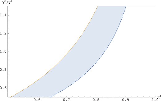
Numerical illustration of a region where the existence condition and the condition for Pareto-improvement are simultaneously satisfied.

Open in new tab Download slide

A close inspection of the figure reveals that, given our parametric assumptions, the information rent effect captured by the denominator of Expression (9) dominates. This is reflected graphically by the fact that the upper boundary is increasing in $π^{1}$ ⁠.²⁷ This implies that, as $π^{1}$ decreases, the government is less likely to attain a Pareto improvement. Of course, this numerical example is purely illustrative and is not meant as an empirical calibration. In the simulations we have chosen a value of η equal to 0.25. The qualitative results in the figure remain robust to the change in the degree of concavity of the function v measured by the constant coefficient of relative risk aversion, $1 - η$ ⁠.

D. Proof of Proposition 2

We begin by proving two lemmas that characterize the optimal duration of parental leave associated with a separating equilibrium and pooling equilibrium, respectively. We then prove Proposition 2 by comparing the social welfare level attained in the optimal separating equilibrium with the social welfare level attained in the optimal pooling equilibrium for each level of the welfare weight β. In all our characterizations we assume that the necessary and sufficient condition for a Pareto-improvement (9) is satisfied.²⁸

Recall that the social maximization problem is defined as follows:

W = max_{j \in {S, P}, \bar{α}} {β U^{1} (\bar{α}, j) + (1 - β) U^{2} (\bar{α}, j)},

where

U^{i} (\bar{α}, j)

denotes the utility derived by a type i worker under an equilibrium of type

j = S, P

(where S denotes the separating and P denotes the pooling equilibrium) when the duration of parental leave is set to

\bar{α}

⁠. The parameter β denotes the weight type 1 workers carry in the social objective function. We also assume that any profits that may arise are taxed away and rebated back to agents in a lump-sum manner, in line with Section 4. To ease but slightly abuse notation, we will drop the second argument j of U in our exposition below, as it will always be obvious which equilibrium regime is under consideration.

Lemma 3.

(Separating Equilibrium).

The optimal solution under the separating regime is given by an interior solution $\bar{α} \in (α^{1 *}, α^{2 *})$ for $γ^{1} < β \leq 1$ and by a corner solution, $\bar{α} = α^{2 *}$ ⁠, for $0 \leq β \leq γ^{1}$ ⁠.
For $\bar{α} \in [α^{1 *}, α^{2 *}], U^{1} (\bar{α})$ is strictly concave and $U^{2} (\bar{α})$ is strictly increasing.
Within the range of an interior solution, the optimal duration of parental leave under a separating equilibrium increases when β decreases.

Proof. Let

U^{i} (\bar{α}), i = 1, 2,

denote the type i workers’ utility level associated with the parental leave rule,

\bar{α}

⁠. By virtue of the definition of the separating equilibrium allocation associated with the parental leave rule,

\bar{α}

(see the proof of Proposition 1 for details), it follows:

U^{1} (\bar{α}) = 1 - π^{1} \bar{α} - \frac{γ^{2}}{γ^{1}} \cdot T (\bar{α}) + π^{1} v (\bar{α}),

U^{2} (\bar{α}) = 1 - π^{2} α^{2 *} + T (\bar{α}) + π^{2} v (α^{2 *}),

where

T (\bar{α}) = γ^{1} (π^{2} α^{2 *} - π^{1} \bar{α} + π^{2} [v (\bar{α}) - v (α^{2 *})])

denotes the universal lump-sum transfer associated with the parental leave rule,

\bar{α}

⁠.

Before turning to formulate the government problem, it is be useful to derive some comparative statics properties of the utility functions,

U^{i} (\bar{α}), i = 1, 2

⁠. We turn first to the utility of type 1 workers. Assuming that the necessary and sufficient condition for a Pareto improvement is satisfied, it follows that

{\frac{\partial U^{1} (\bar{α}))}{\partial \bar{α}} |}_{\bar{α} = α^{1 *}} = v' (α^{1 *}) (π^{1} - γ^{2} π^{2}) - γ^{1} π^{1} > 0.

Namely, starting at the laissez–faire allocation, imposing a binding parental leave rule implies an increase in the utility of type 1 workers. The latter property furthermore implies that

π^{1} - γ^{2} π^{2} > 0

⁠.

By virtue of the fact that

v' (α^{2 *}) = 1

⁠, it follows that

{\frac{\partial U^{1} (\bar{α}))}{\partial \bar{α}} |}_{\bar{α} = α^{2 *}} = v' (α^{2 *}) (π^{1} - γ^{2} π^{2}) - γ^{1} π^{1} = - γ^{2} (π^{2} - π^{1}) < 0.

By virtue of the strict concavity of v it follows hence that there exists a unique value of α, which we denote by

\tilde{α},

which satisfies

{\frac{\partial U^{1} (\bar{α}))}{\partial \bar{α}} |}_{\bar{α} = \tilde{α}} = v' (\tilde{α}) (π^{1} - γ^{2} π^{2}) - γ^{1} π^{1} = 0,

such that for all

α^{1 *} \leq \bar{α} < \tilde{α}

⁠,

\frac{\partial U^{1} (\bar{α}))}{\partial \bar{α}} > 0

⁠, whereas, for all

\tilde{α} < \bar{α} \leq α^{2 *}

⁠,

\frac{\partial U^{1} (\bar{α}))}{\partial \bar{α}} < 0

⁠. We conclude that the utility of type 1 workers is strictly concave in the range

[α^{1 *}, α^{2 *}]

and attains its maximum at

\tilde{α}

⁠.

Turning next to the utility of type 2 workers, it follows that

\frac{\partial U^{2} (\bar{α}))}{\partial \bar{α}} = γ^{1} [π^{2} v' (\bar{α}) - π^{1}] > 0,

for all

α^{1 *} \leq \bar{α} \leq α^{2 *}

⁠, by virtue of the strict concavity of v and as

v' (α^{2 *}) = 1

and

π^{2} > π^{1}

⁠.

The government optimization problem is given by:

max_{\bar{α}} \sum β^{i} U^{i} (\bar{α}),

where

\sum β^{i} = 1

and

0 \leq β^{i} \leq 1

⁠. Formulating the first-order condition with respect to

\bar{α}

yields (where we simplify notation by letting

β^{1} \equiv β) :

\begin{matrix} H (β, \bar{α}) \equiv β \frac{\partial U^{1} (\bar{α}))}{\partial \bar{α}} + (1 - β) \frac{\partial U^{2} (\bar{α}))}{\partial \bar{α}} \\ = β [v' (\bar{α}) (π^{1} - γ^{2} π^{2}) - γ^{1} π^{1}] + (1 - β) γ^{1} [π^{2} v' (\bar{α}) - π^{1}] \geq 0 \\ (= 0, \bar{α} < α^{2 *}) . \end{matrix}

It is straightforward to verify that in case a full weight is assigned to type 1 workers (β = 1) then the optimal solution is interior and given by

\bar{α} = \tilde{α}

⁠. Alternatively, when a full weight is assigned to type 2 workers (β = 0) then the optimum is given by a corner solution,

\bar{α} = α^{2 *}

⁠, and the induced allocation is a pooling equilibrium in which both the duration of parental leave and the compensation is identical for both types of workers. Notice that, by construction, the duration of the parental leave rule under a separating allocation is bounded from above by

α^{2 *}

⁠.

When the optimum is obtained as an interior solution, then by virtue of the first-order condition with respect to $\bar{α}$ ⁠, recalling that $\frac{\partial U^{2} (\bar{α}))}{\partial \bar{α}} > 0$ ⁠, it follows that $\frac{\partial U^{1} (\bar{α}))}{\partial \bar{α}} \leq 0$ ⁠. Thus, $\partial H / \partial β < 0$ ⁠. Moreover, by virtue of the strict concavity of v and the fact that $π^{1} - γ^{2} π^{2} > 0$ ⁠, it follows that $\partial H / \partial \bar{α} < 0$ ⁠. Thus, $\partial \bar{α} / \partial β = - \frac{\partial H / \partial β}{\partial H / \partial \bar{α}} < 0$ ⁠. Hence, within the range of an interior solution, the optimal duration of parental leave is increasing with respect to the weight assigned to type 2 workers (decreasing with respect to β).

As $v' (α^{2 *}) = 1$ and $π^{2} > π^{1}$ ⁠, it is straightforward to verify that $H (1, α^{2 *}) < 0,$ $H (0, α^{2 *}) > 0$ ⁠. Thus, by continuity considerations, the intermediate value theorem implies that there exists some $0 < β < 1$ ⁠, denoted by $\hat{β}$ ⁠, for which $H (\hat{β}, α^{2 *}) = 0$ ⁠. Furthermore, it can be verified that $\frac{\partial H (β, α^{2 *})}{\partial β} = π^{1} - π^{2} < 0$ ⁠, hence, $\hat{β}$ is unique. Substituting for $v' (α^{2 *}) = 1$ into the first-order condition $H (\hat{β}, α^{2 *}) = 0$ ⁠, one can explicitly solve for the cutoff weight, $\hat{β}$ ⁠, to obtain $\hat{β} = γ^{1} .$

Notice finally that as $\partial H / \partial \bar{α} < 0,$ the second-order condition for the government optimization problem is satisfied, so the optimum is indeed characterized by the first-order condition formulated above. □

Lemma 3 highlights the fact that, as the weight β assigned to workers with career orientation decreases (with a corresponding increase in the weight attached to family-oriented workers), the optimal duration of parental leave increases. An increased duration of parental leave induces enhanced cross-subsidization from career-oriented workers toward their family-oriented counterparts. As evident from part (ii) of Lemma 3, an increase in $\bar{α}$ in the interval $[α^{1 *}, α^{2 *}]$ always raises the utility of type 2 workers, and, due to the efficiency-enhancing property of the mandatory parental leave rule, also initially raises the utility of type 1 workers. However, given the concavity of the utility of type 1 workers, a point will eventually be reached where an increase in the utility of type 2 workers comes at the expense of type 1 workers. This trade-off implies the possibility for an interior solution, depending on the value of β. When β is sufficiently small, we get a corner solution and full cross-subsidization in the form of a pooling allocation becomes optimal.²⁹^,³⁰

The next lemma characterizes the pooling regime.

Lemma 4.

(Pooling Equilibrium).

The optimal parental leave $\bar{α}$ under a pooling equilibrium satisfies $\bar{α} > α^{1 *}$ ⁠, increases as β decreases, reaching $\bar{α} = α^{2 *}$ when $β = γ^{1}$ ⁠, and satisfies $\bar{α} > α^{2 *}$ when $0 \leq β < γ^{1}$ ⁠.

Proof. Let $U^{i} (\bar{α}), i = 1, 2,$ denote the type i workers’ utility level associated with the parental leave rule, $\bar{α}$ ⁠. By construction of the mandatory parental leave rule, $\bar{α} \geq α^{1 *}$ ⁠. Furthermore, $U^{i} (\bar{α}) = [1 - \bar{α} (γ^{1} π^{1} + γ^{2} π^{2})] + π^{i} v (\bar{α})$ ⁠, i = 1, 2. Notice that, in contrast to the separating equilibrium, under the pooling regime, expected profits are zero. Thus, there are no tax revenues and the lump-sum transfer is accordingly set to zero. Nonetheless, there is cross-subsidization between the two types of workers, as both receive the same level of compensation, but differ in the expected working time, due to the difference in the propensity of taking up parental leave.

The government optimization problem is given by:

max_{\bar{α}} \sum β^{i} U^{i} (\bar{α}),

where

\sum β^{i} = 1

and

0 \leq β^{i} \leq 1

⁠. Formulating the first-order condition with respect to

\bar{α}

yields (where we again simplify notation by letting

β^{1} \equiv β) :

\begin{matrix} F (β, \bar{α}) \equiv β \frac{\partial U^{1} (\bar{α})}{\partial \bar{α}} + (1 - β) \frac{\partial U^{2} (\bar{α})}{\partial \bar{α}} \\ = - (γ^{1} π^{1} + γ^{2} π^{2}) + [β π^{1} + (1 - β) π^{2}] v' (\bar{α}) \leq 0 (= 0, \bar{α} > α^{1 *}) . \end{matrix}

We first turn to show that, assuming that the necessary and sufficient condition for a Pareto improvement is satisfied, the welfare optimum under a pooling regime is always given by an interior solution; namely,

\bar{α} > α^{1 *}

⁠. To see this, one can re-arrange the first-order condition to establish that a corner solution arises when the following inequality holds:

v' (α^{1 *}) \leq \frac{(γ^{1} π^{1} + γ^{2} π^{2})}{[β π^{1} + (1 - β) π^{2}]} .

At the same time, by virtue of the necessary and sufficient condition for a Pareto improvement, it follows that:

v' (α^{1 *}) > \frac{γ^{1} π^{1}}{(π^{1} - γ^{2} π^{2})} .

To demonstrate that a corner solution cannot exist, it suffices to show that

\frac{γ^{1} π^{1}}{(π^{1} - γ^{2} π^{2})} \geq \frac{(γ^{1} π^{1} + γ^{2} π^{2})}{[β π^{1} + (1 - β) π^{2}]},

which holds if-and-only-if (following some algebraic manipulations),

γ^{1} β {(π^{1})}^{2} + (1 - β) γ^{1} π^{1} π^{2} \geq γ^{1} {(π^{1})}^{2} + {(γ^{2})}^{2} π^{1} π^{2} - {(γ^{2})}^{2} {(π^{2})}^{2} .

Notice that the LHS of the above inequality expression is decreasing with respect to β, as

π^{2} > π^{1}

⁠. Thus, it suffices to prove that the inequality holds for β = 1. Substituting for β = 1 yields upon re-arrangement:

{(γ^{2})}^{2} {(π^{2})}^{2} \geq {(γ^{2})}^{2} π^{1} π^{2}

⁠, which holds as

π^{2} > π^{1}

⁠. This completes the proof.

We conclude that the pooling optimum is given by an interior solution for all values of β.

Finally, notice that for $β = γ^{1}$ ⁠, as $v' (α^{2 *}) = 1$ ⁠, the optimal duration of parental leave is given by $\bar{α} = α^{2 *}$ ⁠. Further notice that by virtue of the strict concavity of v and the fact that $π^{2} > π^{1}$ ⁠, it follows that $\partial F / \partial \bar{α} < 0$ and $\partial F / \partial β < 0$ ⁠. Thus, $\partial \bar{α} / \partial β = - \frac{\partial F / \partial β}{\partial F / \partial \bar{α}} < 0$ ⁠. Hence, the optimal duration of parental leave is increasing with respect to the weight assigned to type 2 workers (decreasing with respect to β).

Notice that as $\partial F / \partial \bar{α} < 0,$ the second-order condition for the government optimization problem is satisfied, so the optimum is indeed characterized by the first-order condition formulated above. □

Lemma 4 states that in the pooling equilibrium, as was the case in the separating regime, it is desirable to set a binding parental leave rule (⁠ $\bar{α} > α^{1 *}$ ⁠). Moreover, as was also the case in the separating equilibrium, the optimal duration of parental leave is an increasing function of the weight assigned to type 2 (family-oriented) workers. Notably, as with the separating regime, a binding parental leave rule is desirable even for the limiting case where a full weight is assigned to type 1 (career-oriented) workers, as it serves to mitigate the distortion associated with the benchmark allocation. The higher the weight assigned to type 2 workers the longer is the duration of the parental leave rule, as the latter serves to enhance the degree of cross-subsidization from type 1 to type 2 workers.

We next combine Lemmas 3 and 4 to prove Proposition 2 and characterize the social optimum as a function of the weight assigned to type 1 (career-oriented) workers, β. We first prove part (ii), then part (i), and finally part (iii).

Part (ii)—Let

W^{sep} (β, \bar{α})

and

W^{pool} (β, \bar{α})

denote, respectively, the welfare levels associated with a separating and a pooling allocation, when the parental leave rule is set at

\bar{α}

and the weight assigned to type 1 workers is β. Further, let

W^{sep} (β)

and

W^{pool} (β)

denote the welfare-maximizing allocations under the separating and the pooling regimes, respectively, when the weight assigned to type 1 workers is β. By virtue of our characterization of the welfare-maximizing allocations under the two regimes, for

β < γ^{1}

⁠, the optimum for the separating regime is given by a corner solution (⁠

\bar{α} = α^{2 *}

⁠) whereas the optimum for the pooling regime is given by an interior solution in which the optimal duration of parental leave satisfies

\bar{α} > α^{2 *}

⁠. Thus, it follows that

W^{pool} (β) > W^{pool} (β, α^{2 *}) = W^{sep} (β, α^{2 *}) = W^{sep} (β) .

Moreover, for

β = γ^{1}

⁠,

W^{pool} (β) = W^{pool} (β, α^{2 *}) = W^{sep} (β, α^{2 *}) = W^{sep} (β) .

This completes the proof of part (ii).

Part (i)—We turn next to prove part (i) by considering the case where

γ^{1} < β \leq 1

⁠. Let

J (β) \equiv W^{sep} (β) - W^{pool} (β)

⁠. Notice that as shown above

J (γ^{1}) = 0

⁠. To complete the proof of part (i) it suffices to show that

J' (β) > 0

for

β > γ^{1}

⁠. Using our previous notation, employing the envelope condition and following some algebraic manipulations, one obtains:

\begin{matrix} J' (β) = \hat{[U^{1}} ({\bar{α}}^{sep}) - \hat{U^{2}} ({\bar{α}}^{sep})] - [U^{1} ({\bar{α}}^{pool}) - U^{2} ({\bar{α}}^{pool})] \\ = (π^{2} - π^{1}) [v ({\bar{α}}^{pool}) - v ({\bar{α}}^{sep}), \end{matrix}

where

{\bar{α}}^{sep}

and

{\bar{α}}^{pool}

denote the optimal duration of parental leave under the separating and the pooling regimes, respectively. As

π^{2} > π^{1}

⁠, to complete the proof of part (i) it suffices to show that

v ({\bar{α}}^{pool}) > v ({\bar{α}}^{sep})

⁠. By virtue of the strict concavity of v it therefore suffices to show that

v' ({\bar{α}}^{pool}) < v' ({\bar{α}}^{sep})

⁠. To see this, we employ the first-order conditions for the welfare optimum under the two regimes to obtain:

v' ({\bar{α}}^{pool}) = \frac{(γ^{1} π^{1} + γ^{2} π^{2})}{[β π^{1} + (1 - β) π^{2}]} and v' ({\bar{α}}^{sep}) = \frac{γ^{1} π^{1}}{β π^{1} + (γ^{1} - β) π^{2}} .

We thus need to show that:

\frac{γ^{1} π^{1}}{β π^{1} + (γ^{1} - β) π^{2}} > \frac{(γ^{1} π^{1} + γ^{2} π^{2})}{[β π^{1} + (1 - β) π^{2}]} .

Re-arranging the LHS of the above inequality yields:

\frac{(γ^{1} π^{1} + γ^{2} π^{2}) - γ^{2} π^{2}}{[β π^{1} + (1 - β) π^{2}] - γ^{2} π^{2}} > \frac{(γ^{1} π^{1} + γ^{2} π^{2})}{[β π^{1} + (1 - β) π^{2}]},

which holds if-and-only-if:

(γ^{1} π^{1} + γ^{2} π^{2}) > [β π^{1} + (1 - β) π^{2}] .

The latter inequality follows as

π^{2} > π^{1}

and

β > γ^{1}

⁠. This completes the proof of part (i).

Part (iii)—Part (iii) follows immediately, by noticing that the optimum is given by an interior solution in both ranges, characterized in parts (i) and (ii) and recalling that within the ranges of the interior solution the optimal duration under both the separating and the pooling regimes is decreasing with respect to β. This completes the proof.

E. Proof of Proposition 3

Notice that by virtue of the binding parental leave mandate, the type 1 zero profit constraint will be slack in the optimal solution for the maximization program in Equation (44). We now show that the incentive constraint for type 2 workers in Equation (44) is binding. To see this, suppose by negation that the constraint is slack. Differentiation of the Lagrange expression in Equation (44) with respect to y¹, assuming that (by our presumption) both constraints are slack (hence

λ = μ = 0

⁠), employing the type 1 worker envelope condition, yields:

\frac{\partial L}{\partial y^{1}} = u' (y^{1} - q π^{1} + T) > 0.

(E.1)

We obtain the desired contradiction to the presumed optimality. It follows that the incentive constraint is necessarily binding in the optimum. Denote by

y^{1} (\bar{α}, T)

the optimal solution for the maximization in Equation (44), given by the implicit solution to the binding incentive constraint:

U^{2 *} (T) = max_{{\hat{π}}^{2}} [u (y^{1} - q {\hat{π}}^{2} + T) + {\hat{π}}^{2} k v (\bar{α})] .

(E.2)

Denoting by

{\hat{U}}^{2} (\bar{α}, T) = {max}_{{\hat{π}}^{2}} [u (y^{1} (\bar{α}, T) - q {\hat{π}}^{2} + T) + {\hat{π}}^{2} k v (\bar{α})]

the RHS of the above equation (the utility derived by a mimicking type 2 worker), it is straightforward to verify, employing the type 2 worker envelope condition, that:

\frac{\partial {\hat{U}}^{2} (\bar{α}, T)}{\partial y^{1}} = u' (y^{1} - q {\hat{π}}^{2} + T) > 0.

(E.3)

Thus, as

U^{2 *} (T)

is independent of y¹, Equation (E.2) uniquely determines

y^{1} (\bar{α}, T)

⁠. Fully differentiating Equation (E.2) with respect to

\bar{α}

and T, employing the type 2 worker envelope conditions and the first-order conditions for the maximization program in Equation (45), yields, upon re-arrangement:

1 + \frac{\partial y^{1} (\bar{α}, T)}{\partial T} = \frac{u' (c^{2})}{(1 + α^{2} \frac{\partial π^{2}}{\partial y^{2}}) u' ({\hat{c}}^{1})} > 0,

(E.4)

where

c^{2} = y^{2} - q π^{2} + T

and

{\hat{c}}^{1} = y^{1} - q {\hat{π}}^{2} + T

⁠. The inequality sign follows by virtue of the maximization of type 2 worker with respect to

π^{2}

⁠, which implies that

q u' (y^{2} - q π^{2} + T) = k v (\bar{α})

⁠, so that

\frac{\partial π^{2}}{\partial y^{2}} = 1 / q > 0

⁠; and,

\frac{\partial y^{1} (\bar{α}, T)}{\partial \bar{α}} = - \frac{{\hat{π}}^{2} k v' (\bar{α})}{u' ({\hat{c}}^{1})} < 0.

(E.5)

We turn next to show that the revenue constraint in the maximization program given in Equation (46) is binding in the optimum. To see this, suppose by negation that the constraint is slack (hence

ϕ = 0

⁠). Differentiating

U^{1} (\bar{α}, T)

with respect to T, employing the type 1 worker envelope condition, yields:

\frac{\partial U^{1} (\bar{α}, T)}{\partial T} = u' (c^{1}) (1 + \frac{\partial y^{1}}{\partial T}) > 0,

(E.6)

where

c^{1} = y^{1} - q π^{1} + T

⁠, and where the inequality sign follows from Equation (E.4). Thus, we obtain the desired contradiction to the presumed optimality. We therefore conclude that the revenue constraint is binding in the optimum. For each duration of parental leave,

\bar{α}

⁠, the level of transfer,

T (\bar{α})

⁠, is given by the implicit solution to the binding revenue constraint, namely:

G (\bar{α}, T) \equiv 1 - π^{1} \bar{α} - y^{1} - T / γ^{1} = 0.

(E.7)

Differentiating G with respect to T, yields upon re-arrangement:

\frac{\partial G}{\partial T} = - (1 + \frac{\partial y^{1}}{\partial T}) (1 + \bar{α} \frac{\partial π^{1}}{\partial y^{1}}) - \frac{γ^{2}}{γ^{1}} < 0,

(E.8)

where the inequality sign follows from Equation (E.4) and by virtue of the maximization of type 1 worker with respect to

π^{1}

⁠, which states that

q u' (y^{1} - q π^{1} + T) = v (\bar{α})

⁠, so that

\frac{\partial π^{1}}{\partial y^{1}} = 1 / q > 0

⁠. We thus conclude that

T (\bar{α})

is uniquely determined. By construction,

T (\bar{α}) \to 0

\bar{α} \to α^{1 *}

⁠; namely, the extent of cross-subsidization from type 1 to type 2 workers converges to zero as we approach the laissez–faire equilibrium.

The maximization program in Equation (46) can be re-formulated as:

max_{\bar{α}} H (\bar{α}),

(E.9)

where

H (\bar{α}) \equiv U^{1} [\bar{α}, T (\bar{α})]

and

T (\bar{α})

are given by the implicit solution to Equation (E.7).

Assuming that the second-order condition for the maximization in Equation (E.9) is satisfied, a necessary and sufficient condition for a Pareto improvement is:

{\frac{\partial H}{\partial \bar{α}} |}_{\bar{α} = α^{1 *}, T = 0} = {\frac{\partial U^{1}}{\partial \bar{α}} |}_{\bar{α} = α^{1 *}, T = 0} + {[\frac{\partial U^{1}}{\partial T} \cdot \frac{\partial T}{\partial \bar{α}}] |}_{\bar{α} = α^{1 *,}, T = 0} > 0.

(E.10)

That is, starting at the laissez–faire allocation, setting a slightly binding parental leave rule (supplemented by a confiscatory profit tax and a uniform lump-sum transfer) increases the utility of type 1 workers.

Differentiation of

U^{1} (\bar{α}, T)

with respect to

\bar{α}

and T, employing type 1 worker envelope condition and evaluating the expressions at the laissez–faire allocation levels, yields:

{\frac{\partial U^{1}}{\partial \bar{α}} |}_{\bar{α} = α^{1 *}, T = 0} = {u (c^{1 *}) \frac{\partial y^{1}}{\partial \bar{α}} |}_{\bar{α} = α^{1 *}, T = 0} + π^{1 *} v^{'} (α^{1 *})

(E.11)

and

{\frac{\partial U^{1}}{\partial T} |}_{\bar{α} = α^{1 *}, T = 0} = u (c^{1 *}) (1 + \frac{\partial y^{1}}{\partial T} |_{\bar{α} = α^{1 *}, T = 0}),

(E.12)

where

c^{1 *} = y^{1 *} - q π^{1 *}

⁠.

Differentiating G, given in Equation (E.7), with respect to

\bar{α}

⁠, yields upon re-arrangement:

\frac{\partial G}{\partial \bar{α}} = - [π^{1} + \bar{α} \frac{\partial π^{1}}{\partial \bar{α}} + \frac{\partial y^{1}}{\partial \bar{α}} (1 + \bar{α} \frac{\partial π^{1}}{\partial y^{1}})] .

(E.13)

Thus, by virtue of Equation (E.8), it follows that:

\begin{matrix} {\frac{\partial T}{\partial \bar{α}} |}_{\bar{α} = α^{1 *}, T = 0} = - {\frac{\frac{\partial G}{\partial \bar{α}}}{\frac{\partial G}{\partial T}} |}_{\bar{α} = α^{1 *}, T = 0} = \\ - \frac{[π^{1 *} + {α^{1 *} \frac{\partial π^{1}}{\partial \bar{α}} |}_{\bar{α} = α^{1 *}, T = 0} + {\frac{\partial y^{1}}{\partial \bar{α}} |}_{\bar{α} = α^{1 *}, T = 0} (1 + {α^{1 *} \frac{\partial π^{1}}{\partial y^{1}} |}_{\bar{α} = α^{1 *}, T = 0})]}{(1 + {\frac{\partial y^{1}}{\partial T} |}_{\bar{α} = α^{1 *}, T = 0}) (1 + {α^{1 *} \frac{\partial π^{1}}{\partial y^{1}} |}_{\bar{α} = α^{1 *}, T = 0}) - \frac{γ^{2}}{γ^{1}}} . \end{matrix}

(E.14)

Substitution for

{\frac{\partial U^{1}}{\partial \bar{α}} |}_{\bar{α} = α^{1 *}, T = 0}

⁠,

{\frac{\partial U^{1}}{\partial T} |}_{\bar{α} = α^{1 *}, T = 0}

⁠, and

{\frac{\partial T}{\partial \bar{α}} |}_{\bar{α} = α^{1 *}, T = 0}

from Equations (E.11), (E.12), and (E.14) into Equation (E.10) employing Equations (41), (42), (E.4), and (E.5), yields upon re-arrangement (we abbreviate notation by referring to all derivatives as evaluated at the laissez–faire levels):

{\frac{\partial H}{\partial \bar{α}} |}_{\bar{α} = α^{1 *}, T = 0} > 0 \Leftrightarrow \frac{\frac{u^{'} (c^{2 *}) (1 + α^{1 *} \frac{\partial π^{1}}{\partial y^{1}})}{1 + α^{2 *} \frac{\partial π^{2}}{\partial y^{2}}} [\frac{π^{1 *} v^{'} (α^{1 *}) q}{v (α^{1 *})} - \frac{π^{1 *} + α^{1 *} \frac{\partial π^{1}}{\partial \bar{α}}}{1 + α^{1 *} \frac{\partial π^{1}}{\partial y^{1}}}]}{k v^{'} (α^{1 *}) \cdot ({\hat{π}}^{2 *} - π^{1 *})} > \frac{γ^{2}}{γ^{1}} .

(E.15)

Finally, taking into account that the derivative of πⁱ w.r.t yⁱ is equal to

1 / q

⁠, one obtains Equation (47).

F. The Role of Subsidized Leave

Suppose that the government provides a flat subsidized parental leave system, which takes the form: $G^{i} = b π^{i},$ i = 1, 2, where b > 0. We will characterize the modified necessary and sufficient condition for attaining a Pareto improvement. We then demonstrate that the set of parameters for which a Pareto improvement is attained is a subset of the corresponding set for the regime with a universal transfer. Thus, providing a subsidized scheme which depends on the time spent on leave, rather than a universal system, results in a shrinkage of the set of parameters for which a Pareto improvement can be obtained.

A separating equilibrium allocation associated with a mandatory parental leave rule

\bar{α}, α^{1 *} \leq \bar{α} < α^{2 *}

⁠, supplemented by a confiscatory tax levied on pure profits, T, and a flat subsidized transfer, b, is given by:

{α^{i}, y^{i}}_{i = 1, 2}, T, b,

where:

y^{i} = 1 - π^{i} α^{i}; i = 1, 2,

(F.1)

α^{1} = \bar{α},

(F.2)

α^{2} = α^{2 *} where v' (α^{2 *}) = 1,

(F.3)

y^{2} + b π^{2} + π^{2} v (α^{2}) = y^{1} - T + b π^{2} + π^{2} v (α^{1}),

(F.4)

γ^{1} T = b \cdot (γ^{1} π^{1} + γ^{2} π^{2}) .

(F.5)

Substituting for αⁱ and yⁱ, i = 1, 2, from Conditions (F.1)–(F.3) into Condition (F.4) and re-arranging, yields:

T (\bar{α}) = π^{2} α^{2 *} - π^{1} \bar{α} + π^{2} [v (\bar{α}) - v (α^{2 *})]

⁠. Notice that

T (α^{1 *}) = 0

by construction of the laissez–faire equilibrium. Further notice that T is strictly increasing with respect to

\bar{α}

⁠, by virtue of the strict concavity of v and the fact that

\bar{α} \leq α^{2 *}, v' (α^{2 *}) = 1

and

π^{2} > π^{1} .

Thus,

T (\bar{α}) > 0

for all

\bar{α} > α^{1 *}

⁠.

Let

\hat{U^{1}} (\bar{α})

denote the utility derived by type 1 workers in the separating equilibrium associated with the parental leave rule,

\bar{α}

⁠. Formally,

\hat{U^{1}} (\bar{α}) = 1 - π^{1} \bar{α} - T (\bar{α}) + b π^{1} + π^{1} v (\bar{α})

⁠. Substituting for

T (\bar{α})

into (v) yields:

b (\bar{α}) = γ^{1} T (\bar{α}) / (γ^{1} π^{1} + γ^{2} π^{2})

⁠. Substituting for

T (\bar{α})

and

b (\bar{α})

into

\hat{U^{1}} (\bar{α})

yields upon re-arrangement:

\hat{U^{1}} (\bar{α}) = 1 - π^{1} \bar{α} + π^{1} v (\bar{α}) - (π^{2} α^{2 *} - π^{1} \bar{α} + π^{2} [v (\bar{α}) - v (α^{2 *})]) \cdot \frac{γ^{2} π^{2}}{γ^{1} π^{1} + γ^{2} π^{2}} .

By a similar reasoning to the one provided in the proof of Proposition 1, a necessary and sufficient condition for a Pareto improvement under the flat subsidized system is

{\frac{\partial \hat{U^{1}} (\bar{α}))}{\partial \bar{α}} |}_{\bar{α} = α^{1 *}} > 0

⁠. Differentiation of

\hat{U^{1}} (\bar{α})

with respect to

\bar{α},

evaluating the derivative at

\bar{α} = α^{1 *}

⁠, yields upon rearrangement:

{\frac{\partial \hat{U^{1}} (\bar{α}))}{\partial \bar{α}} |}_{\bar{α} = α^{1 *}} > 0 \Leftrightarrow γ^{2} / γ^{1} < \frac{[v' (α^{1 *}) - 1]}{v' (α^{1 *}) \cdot (\frac{π^{2}}{π^{1}} - 1) \cdot \frac{π^{2}}{π^{1}}} .

The necessary and sufficient condition for the universal transfer regime, stated in Proposition 1, is given by

γ^{2} / γ^{1} < \frac{[v' (α^{1 *}) - 1]}{v' (α^{1 *}) \cdot (\frac{π^{2}}{π^{1}} - 1)} .

Comparing the two inequality conditions, recalling that

π^{2} > π^{1},

implies that the set of parameters for which a Pareto improvement is attained under the flat subsidized regime is indeed a subset of the set of parameters for which a Pareto improvement is attained under the universal transfer regime. This establishes our argument. A similar procedure can be applied to show that the set of parameters for which a Pareto improvement can be obtained also shrinks when the subsidized parental leave system takes the form

G^{i} = b π^{i} α^{i},

i = 1, 2, where b > 0.

Conflict of interest statement. None declared.

Acknowledgement

A previous version of this paper circulated under the title, ‘Anti-discrimination legislation and the efficiency-enhancing role of mandatory parental leave’. We are grateful to two anonymous referees, as well as Dan Anderberg, Katherine Cuff, Thomas Giebe, Nils Gottfries, Oskar Nordström-Skans, Dan-Olof Rooth, and seminar participants at the NORFACE Welfare State Futures Conference, The Uppsala Center for Labor Studies (UCLS) Annual Members Meeting, the CESifo Employment and Social Protection Conference, the International Institute of Public Finance Annual Meeting in Lake Tahoe, the Association for Public Economic Theory Annual Meeting in Paris, the Annual Meeting of the Israeli Economics Association in Tel Aviv, Umeå University, Linnaeus University, University of Siegen, University of Bologna, Bocconi University of Milan, and the Research Institute for Industrial Economics (IFN) in Stockholm for helpful comments on an earlier draft of the paper. Financial Support from Riksbankens Jubileumfond and the Jan Wallander and Tom Hedelius Foundation is gratefully acknowledged.

Footnotes

1. See Bertrand et al. (2010) who focus on workers in the corporate and financial sector. Bertrand et al. (2010) also present suggestive evidence using data from the Harvard and Beyond (H&B) project showing that female MBAs appear to have a more difficult time combining career and family than do, for example, female physicians. Further evidence on the important effects of child-related absences on labor market outcomes is presented by Angelov et al. (2016).

2. A country with one of the world’s most generous systems is Sweden where each parent has the legal right to be absent from work until the child is 18 months old. In total, Swedish parents are entitled to 480 days of government subsidized parental leave. Unclaimed days can be saved, and used for parental leave spells up until the child is 8 years old. This is supplemented by generous sick-leave arrangements allowing parents to take up to 120 days off work per year for each sick child under the age of 12 years. In addition, parents in Sweden have the right to work 75% out of the normal (full-time) weekly working hours until the child is 8 years old.

3. Although they do not model the behavior of firms in their theoretical analysis.

4. Using data from the United States, she shows that such policies increase female employment but decrease the likelihood of women getting promoted.

5. Using her calibrated model, she performs simulations of different policies, including family-friendly policies such as paid parental leave, part-time work entitlements, and subsidized child care, noticing sometimes ambiguous effects these policies can have on gender equality in the labor market.

6. We discuss the separability of the utility function in footnote 25 on page 31 in that section.

7. As we have decided to focus on gender-related issues, we have refrained from explicitly modeling these other dimensions of heterogeneity which are also likely to be correlated with career/family orientation.

8. Notice that becoming less productive per unit of time is likely to be largely determined by having a low degree of workplace attendance in earlier time periods. This is the mechanism of human capital accumulation emphasized in Bronson (2015) and Blundell et al. (2016). Thus, one can interpret (2) as not only reflecting the instantaneous loss in output due to workplace absence, but also the expected productivity losses tomorrow due to a higher workplace absence today.

9. We follow the notion of equilibrium suggested by the seminal paper by Rothschild and Stiglitz (1976).

10. A separating equilibrium exists as long as the pooling line (i.e., the zero-profit line that would be relevant to firms hiring both types of workers), represented by the dotted line in Figure 2, lies below the indifference curve of type 1 workers (as is the case in the figure). The issue of the existence of a separating equilibrium is discussed in the end of this section and further explored in Section 6.

11. To see this formally, note that under full information, by virtue of Condition (3), the allocation of type 1 workers satisfies $v' (α^{1}) = 1$ whereas in the presence of asymmetric information the allocation of type 1 workers is distorted, implying that $v' (α^{1}) > 1$ ⁠. The result then follows by the strict concavity of v.

12. In the ‘first best’ sense, as demonstrated above, the benchmark allocation is inefficient. Our purpose, however, is to examine whether the benchmark equilibrium is second-best inefficient given the policy tools available to the government.

13. Notice that Condition (8) is not equivalent to Assumption 1, invoked to imply that a separating equilibrium exists, due to the tax system in place. Nonetheless, Assumption 1 implies that Equation (8) is satisfied, by continuity, provided that the degree of cross-subsidization induced by imposing the binding parental leave rule is sufficiently small.

14. Provided that this ratio does not fall below a certain threshold so that the separating equilibrium ceases to exist, see the discussion below and Appendix C.

15. This is shown in Appendix B where we also resolve this ambiguity in a numerical example given certain parametric assumptions.

16. A pooling equilibrium supported by a parental leave rule can however be optimal from a social welfare perspective, as demonstrated in Section 5.

17. According to an analysis by the International Labor Organization of the United Nations, 74 out of 167 countries with available data provide maternity benefits that amount to at least two-thirds of a woman’s previous earnings for at least 14 weeks. Out of them, 61 countries provide 100% of prior earnings for 14 weeks (see Rossin-Slater 2017).

18. As mentioned earlier on, one way to interpret π is as the expected number of children, in which case subsidized parental leave is equivalent to child benefits. In a working paper version of this paper (Bastani et al. 2016, Appendix C), we show that allowing to tax children (rather than providing benefits) can expand the set of parameters for which a Pareto improvement can be obtained. The potentially welfare-enhancing role of taxing children has previously been emphasized by Balestrino et al. (2002) and Cigno and Pettini (2002).

19. We would like to make a remark on the issue of implementability. Notice that when β is sufficiently low, the social optimum is a pooling allocation with $\bar{α} > α^{2 *}$ ⁠. For such values of $\bar{α}$ ⁠, a separating equilibrium cannot exist. However, in the case with a high β, $\bar{α} < α^{2 *}$ and both the separating and pooling allocation can co-exist. Therefore, in order to achieve full implementation of the separating allocation, one needs to ensure that a pooling allocation cannot form an equilibrium. One way to do this would be to impose a 100% confiscatory income tax on the income level associated with the pooling allocation.

20. Notice that relative to the symmetric information equilibrium, there is a difference in the consumption allocation due to the induced cross-subsidization in the parental leave regime. However, due to quasi-linearity, the government is indifferent to how consumption is divided between the two types of workers in this case.

21. The result that gender wage gaps are fully eliminated is driven by the fact that in the symmetric information efficient allocation, both types of workers are prescribed the same duration of parental leave. Modifying our framework, by assuming either that family-oriented workers derive a higher utility from being absent from work than their career-oriented counterparts, or, that workers choosing the career-track are more productive, per unit of time spent working, than equally skilled workers opting for the family track, will change this result. In particular, it will imply that in a symmetric information efficient allocation, contracts offered to family-oriented workers will prescribe a longer duration of parental leave, relative to the contracts offered to career-oriented workers. In this case, there will be a threshold $\bar{β}$ ⁠, satisfying $0 < \bar{β} < γ^{1}$ ⁠, such that for β exceeding this threshold, the social optimum will be given by a separating allocation, whereas for β below this threshold, a pooling allocation will be socially optimal. When a separating allocation is socially optimal, the parental leave policy would mitigate rather than fully eliminate the gender wage gap.

22. For tractability, we focus on the quasi-linear case. This is without loss of generality for the purpose of showing that the incentive constraint binds. The reason is that with nonlinear utility of consumption, there would be an income effect working in the direction of making the difference in α between the two types of agents less pronounced in the symmetric information equilibrium. Hence, having nonlinear utility of consumption would just make it more likely that the incentive constraint is binding.

23. To see this formally, notice that Equation (43) can be written as $\frac{π^{1} q v' (α^{1})}{v (α^{1})} \cdot \frac{1 - δ μ k}{1 - μ k} - \frac{π^{1} + α^{1} \frac{\partial π^{1}}{\partial α^{1}}}{1 + α^{1} \frac{\partial π^{1}}{\partial y^{1}}} = 0$ ⁠. This can be interpreted as a first-order condition along the envelope (when all else has been chosen optimally by the firm and by the workers). Then it follows that $\frac{π^{1} q v' (α^{1})}{v (α^{1})} > \frac{π^{1} + α^{1} \frac{\partial π^{1}}{\partial α^{1}}}{1 + α^{1} \frac{\partial π^{1}}{\partial y^{1}}}$ since $\frac{1 - δ μ k}{1 - μ k} < 1$ ⁠. Comparing this with Equation (36) (in which the two terms are equalized) assuming that the second-order conditions are satisfied, implies that the $α^{1}$ under the asymmetric information case (for which we obtain an inequality) is lower than the $α^{1}$ under the symmetric information case (for which we obtain an equality). This is because the derivative is positive at $α^{1}$ in the asymmetric information allocation and hence the optimal choice of α under the symmetric information case should be higher (in order to obtain an equality, i.e., the first order condition).

24. This is shown in Appendix E.

25. Qualitatively similar results would be obtained assuming non-separability between consumption and other arguments in the utility function. Glancing at Equation (47), non-separability would imply two main differences: (i) in the numerator of the expression in curly brackets the first term would become the type 1 marginal rate of substitution between α and y (⁠ ${MRS}_{α, y}$ defined as the ratio between the derivative of the individual indirect utility function with respect to α and the derivative with respect to y), (ii) at the denominator we would have the product between the marginal utility of consumption for a type 2 mimicker and the difference between ${MRS}_{α, y}$ for a type 2 mimicker and a type 1 agent. Thus, qualitatively similar results would be obtained as long as ${MRS}_{α, y}$ is larger for a type 2 mimicker when compared with a type 1 agent at all points in the $(α, y)$ -space.

26. Notice that according to our parametric specification, the necessary and sufficient condition (B.5) for a Pareto improvement to exist is homogeneous in the ratio $π^{1} / π^{2}$ ⁠. Thus, the fact that we fixed $π^{2}$ and conducted the comparative statics with respect to $π^{1}$ is of no substance for the qualitative results, provided that we satisfy the existence condition.

27. To see this, consider Equation (9) satisfied as an equality. The upward slope of the upper curve in Figure 5 implies that the RHS of Condition (9) is increasing in $π^{1}$ ⁠. As we already demonstrated that both the numerator and denominator of the RHS of Equation (9) are decreasing in $π^{1}$ ⁠, this implies that the effect associated with the denominator is prevailing.

28. This assumption is not necessary but is made for simplicity. We comment on how it affects the results in footnote 29.

29. As mentioned on page 39, in our derivations we assume that the necessary and sufficient condition for Pareto improvement is satisfied. Without this assumption the characterization in Lemma 3 would be qualitatively similar, barring the fact that the utility of type 1 would be monotonically decreasing with respect to the parental leave duration, and that, for high enough β, the optimum would be non-intervention (not setting a binding parental leave rule).

30. Notice that we have, just as in Section 4, confined attention to the case where tax revenues (from the pure profits taxation of firms employing type 1 workers) are rebated via a uniform lump-sum transfer. Allowing for subsidized parental leave (see our discussion in Section 4.3) would further enhance the government capacity to redistribute from type 1 to type 2 workers. We then anticipate that the government will increase the generosity of the subsidized parental leave system as the weight assigned to family-oriented workers increases (alongside extending the duration of the parental leave). When full weight is assigned to career-oriented workers, there will be nothing to gain from a subsidized parental leave structure, though, and the optimal system will remain one in which a universal lump-sum transfer is paid to both types of workers.

References

Angelov

Johansson

Lindahl

2016

“Parenthood and the Gender Gap in Pay,”

Journal of Labor Economics

545

–

Google Scholar

Crossref

WorldCat

Balestrino

Cigno

Pettini

2002

“Endogenous Fertility and the Design of Family Taxation,”

International Tax and Public Finance

175

–

Google Scholar

Crossref

WorldCat

Barigozzi

Cremer

Roeder

2017

. “Women’s career choices, social norms and child care policies.” IZA Discussion Paper No. 10502.

Bastani

Blumkin

Micheletto

2015

“Optimal Wage Redistribution in the Presence of Adverse Selection in the Labor Market,”

131

Journal of Public Economics

–

Google Scholar

Crossref

WorldCat

Bastani

Blumkin

Micheletto

2016

. “Anti-discrimination Legislation and the Efficiency-Enhancing Role of Mandatory Parental Leave.” CESifo Working Paper No. 5917.

Bertrand

Goldin

Katz

L. F.

2010

“Dynamics of the Gender Gap for Young Professionals in the Financial and Corporate Sectors,”

American Economic Journal: Applied Economics

228

–

Google Scholar

Crossref

WorldCat

Blau

F. D.

Kahn

L. M.

2013

“Female Labor Supply: Why Is the US Falling behind?,”

103

The American Economic Review

251

–

Google Scholar

Crossref

WorldCat

Blundell

Costa Dias

Meghir

Shaw

2016

“Female Labor Supply, Human Capital, and Welfare Reform,”

Econometrica

1705

–

Google Scholar

Crossref

WorldCat

Bronson

M. A.

2015

. “Degrees Are Forever: Marriage, Educational Investment, and Lifecycle Labor Decisions of Men and Women.” Mimeo, Georgetown University.

Budig

M. J.

England

2001

“The Wage Penalty for Motherhood,”

American Sociological Review

2004

–

225

Google Scholar

Crossref

WorldCat

Chan

Eyster

2003

“Does Banning Affirmative Action Lower College Student Quality?,”

American Economic Review

858

–

Google Scholar

Crossref

WorldCat

Cigno

Pettini

2002

“Taxing Family Size and Subsidizing Child-Specific Commodities?,”

Journal of Public Economics

–

Google Scholar

Crossref

WorldCat

Cremer

Roeder

2017

“Social Insurance with Competitive Insurance Markets and Risk Misperception,”

146

Journal of Public Economics

138

–

Google Scholar

Crossref

WorldCat

Del Rey

Racionero

Silva

J. I.

2017

“On the Effect of Parental Leave Duration on Unemployment and Wages,”

158

Economics Letters

–

Google Scholar

Crossref

WorldCat

Eckstein

Eichenbaum

Peled

1985

“Uncertain Lifetimes and the Welfare Enhancing Properties of Annuity Markets and Social Security,”

Journal of Public Economics

303

–

Google Scholar

Crossref

WorldCat

Encinosa

2001

“A Comment on Neudeck and Podczeck’s ‘Adverse Selection and Regulation in Health Insurance Markets’,”

Journal of Health Economics

667

–

Finkelstein

2004

“Minimum Standards, Insurance Regulation and Adverse Selection: Evidence from the Medigap Market,”

Journal of Public Economics

2515

–

Google Scholar

Crossref

WorldCat

Fryer

R. G.

Loury

G. C.

Yuret

2008

“An Economic Analysis of Color-Blind Affirmative Action,”

Journal of Law, Economics, and Organization

319

–

Google Scholar

Crossref

WorldCat

Goldin

2014

“A Grand Gender Convergence: Its Last Chapter,”

104

American Economic Review

1091

–

119

Google Scholar

Crossref

WorldCat

Hackmann

M. B.

Kolstad

J. T.

Kowalski

A. E.

2015

“Adverse Selection and an Individual Mandate: When Theory Meets Practice,”

105

American Economic Review

1030

–

McFadden

Noton

Olivella

2015

“Minimum Coverage Regulation in Insurance Markets,”

SERIEs

247

–

Google Scholar

Crossref

WorldCat

Neudeck

Podczeck

1996

“Adverse Selection and Regulation in Health Insurance Markets,”

Journal of Health Economics

387

–

408

Olivetti

Petrongolo

2016

“The Evolution of Gender Gaps in Industrialized Countries,”

Annual Review of Economics

405

–

Google Scholar

Crossref

WorldCat

Pichler

Ziebarth

N. R.

2017

“The Pros and Cons of Sick Pay Schemes: Testing for Contagious Presenteeism and Noncontagious Absenteeism Behavior,”

156

Journal of Public Economics

–

Google Scholar

Crossref

WorldCat

Rossin-Slater

2017

. “Maternity and Family Leave Policy.” NBER Working Paper No. 23069.

Rothschild

Stiglitz

1976

“Equilibrium in Competitive Insurance Markets: An Essay on the Economics of Imperfect Information,”

Quarterly Journal of Economics

629

–

Google Scholar

Crossref

WorldCat

Stantcheva

2014

“Optimal Income Taxation with Adverse Selection in the Labor Market,”

Review of Economic Studies

1296

–

329

Google Scholar

Crossref

WorldCat

Summers

L. H.

1989

“Some Simple Economics of Mandated Benefits,”

American Economic Review Papers and Proceedings

177

–

Google Scholar

OpenURL Placeholder Text

WorldCat

Thomas

2018

. “The Impact of Mandated Maternity Benefits on the Gender Differential in Promotions: Examining the Role of Adverse Selection.” Mimeo, Cornell University.

Waldfogel

1997

“The Effect of Children on Women’s Wages,”

American Sociological Review

209

–

Google Scholar

Crossref

WorldCat

This is an Open Access article distributed under the terms of the Creative Commons Attribution-NonCommercial-NoDerivs licence (http://creativecommons.org/licenses/by-nc-nd/4.0/), which permits non-commercial reproduction and distribution of the work, in any medium, provided the original work is not altered or transformed in any way, and that the work is properly cited. For commercial re-use, please [email protected]

Download all slides

Month:	Total Views:
November 2018	40
December 2018	42
January 2019	44
February 2019	134
March 2019	110
April 2019	64
May 2019	82
June 2019	56
July 2019	58
August 2019	37
September 2019	40
October 2019	64
November 2019	34
December 2019	13
January 2020	25
February 2020	34
March 2020	45
April 2020	28
May 2020	21
June 2020	30
July 2020	27
August 2020	16
September 2020	28
October 2020	28
November 2020	27
December 2020	20
January 2021	18
February 2021	18
March 2021	27
April 2021	26
May 2021	25
June 2021	14
July 2021	20
August 2021	14
September 2021	15
October 2021	25
November 2021	53
December 2021	155
January 2022	139
February 2022	123
March 2022	120
April 2022	125
May 2022	119
June 2022	105
July 2022	110
August 2022	99
September 2022	124
October 2022	100
November 2022	111
December 2022	106
January 2023	93
February 2023	103
March 2023	109
April 2023	98
May 2023	92
June 2023	82
July 2023	99
August 2023	116
September 2023	104
October 2023	107
November 2023	131
December 2023	103
January 2024	104
February 2024	99
March 2024	111
April 2024	160
May 2024	110
June 2024	31
July 2024	28
August 2024	34
September 2024	30
October 2024	29
November 2024	49
December 2024	32
January 2025	29
February 2025	28
March 2025	35
April 2025	4
May 2025	3

Article Contents

The Welfare-Enhancing Role of Parental Leave Mandates

Abstract

1. Introduction

2. Related Literature

3. Model

3.1 Symmetric Information Equilibrium

3.2 Benchmark Equilibrium with Asymmetric Information

3.3 The Gender Wage Gap in the Benchmark Equilibrium

4. The Efficiency-Enhancing Role of Parental Leave

4.1 Equilibrium in the Presence of a Parental Leave Mandate

4.2 When Is Parental Leave Efficiency Enhancing?

4.3 Subsidized Parental Leave

5. The Socially Desirable Duration of Parental Leave

5.1 Characterization of the Second Best Pareto Frontier and Implications for Gender Equality

6. Extensions

6.1 Endogenous π and Quasi-Linear Utility

6.1.1 Incentive Incompatibility of the Symmetric Information Equilibrium

6.2 A Simple Model with Productivity Differences

6.2.1 Symmetric Information Equilibrium

6.2.2 Incentive Incompatibility of the Symmetric Information Equilibrium

6.3 Endogenous π and Non-linear Utility of Consumption

6.3.1 The Symmetric Information Case

6.3.2 The Asymmetric Information Case

6.3.3 Equilibrium with Parental Leave Mandate

6.3.4 Subsidizing Child Care Costs

7. Conclusions

A. Proof of Proposition 1

B. Comparative Statics with Respect to π

C. Numerical Example

C.1 Existence of a Pareto-Improving Allocation

C.2 Existence of a Separating Equilibrium

D. Proof of Proposition 2

E. Proof of Proposition 3

F. The Role of Subsidized Leave

Acknowledgement

Footnotes

References

Citations

Views

Altmetric

Email alerts

Citing articles via

Latest

Most Read

Most Cited

This Feature Is Available To Subscribers Only