


Abstract
The use of batteries became essential in our daily life in electronic devices, electric vehicles and energy storage systems in general terms. As they play a key role in many devices, their design and implementation must follow a thorough test process to check their features at different operating points. In this circumstance, the appearance of any kind of deviation from the expected operation must be detected. This research deals with real data registered during the testing phase of a lithium iron phosphate—LiFePO4—battery. The process is divided into four different working points, alternating charging, discharging and resting periods. This work proposes a hybrid classifier, based on one-class techniques, whose aim is to detect anomalous situations during the battery test. The faults are created by modifying the measured cell temperature a slight ratio from their real value. A detailed analysis of each technique performance is presented. The average performance of the chosen classifier presents successful results.
1 Introduction
The increasing concern about the environmental impact caused by greenhouse gases emission has resulted in the development of policies that seek to palliate this situation [14]. In this context, many efforts are focused on the promotion of electric vehicles technology. From 2012 to 2018, the number of electric vehicles has been multiplied by 30 [15]. Nowadays, one of the main problems with electric vehicles is the driving range, which is directly linked with the storage system. Then, in the race for improving electric vehicles, the quality and features of batteries are crucial.
However, the use of batteries is important not only in the electric mobility field. It can solve the problem of intermittent energy generation from renewable sources, by storing energy to avoid power cuts [12]. In this field, the batteries are able to save electrical energy if the generation is greater than the demand and, then, they can give back this saved energy in case the demand exceeds the production. It is also important to remark that this application is also extremely related to the reduction of environmental impact caused by fossil fuels [12]. This global trend shows that batteries represent a significant piece to build a sustainable future. Hence, the research community has focused their interests on the improvement of electrical energy storage systems. The implementation of smart grids to efficiently manage the energy produced by wind or solar power systems is presented as a feasible alternative to the power grid structure [25].
Besides the energy storage systems for renewable energies and the electric vehicles, the portable electronic devices, such as laptops, headphones or cellphones, are also demanding greater autonomy, fast charging and less weight and power losses [11].
From a technical point of view, the battery operation is based on electric and chemical reactions. The battery features depend on the chemical elements present in it. In this case, a lithium iron phosphate—LiFePO4—(LFP) power cell is studied, whose use is very common in electric vehicles. Some of the reasons for its wide-spread use are its high voltage, great power density, low self-discharge, long service life and no memory effect [16].
The positive features described above, along with the wide variety of applications where the batteries are essential, emphasize the importance of ensuring their optimum performance. Then, during the test process, it is mandatory to determine the correct operation and the lack of degradation. From a given application, anomalies [29], also known as outliers [26] or novelties [4], can be defined as instances that present an unexpected behaviour [10].
In [7], a virtual sensor to predict the state of charge (SOC) of an LFP power cell is implemented. This is carried out using artificial neural networks and support vector regression, combined with clustering algorithms. This kind of research is not only focused on LFP power cells. In [9], a hydrogen-based fuel cell is modelled to predict the dynamic behaviour during normal operation. A hybrid topology is also considered to predict the voltage value of the cell, achieving good performance in the prediction. In [3], the hydrogen flow is modelled through a similar approach, to tackle the problem of nonlinearity in hydrogen-based fuel cells. These works emphasize the idea of the importance of grouping the dataset prior to the model stage.
The use of this virtual sensor could represent an interesting tool to determine anomalies. However, this idea presents a critical weakness, which is the need of the previous system knowledge, necessary to determine the normal operating range of a battery. The need of a fault criteria is one of the motivations of the present work.
Hence, the main idea of this work is to implement an unsupervised system capable of detecting anomalies. To do so, the use of one-class techniques has shown a really good performance in a wide variety of fields, such as industry or medicine [8, 18, 21]. The main basis of one-class techniques rests on the fact that only information about correct operation is available [29]. Then, instances that do not belong to the known class are labelled as anomalies.
This work deals with the anomaly detection in a LFP power cell during the test stage. As this process is commonly divided into four phases, a one-class classifier for each phase is implemented. Different techniques are tested over each phase with the aim of achieve the best performance. Given the unfeasibility of having real data from anomalous situations, they are artificially generated by modifying different percentages the battery temperatures: 5%, 10%, 15% and 20%.
This paper is structured as follows: after the introduction section, the LFP power cell is described in next section. Then, the techniques applied are detailed in Section 3. Section 4 describes the experiments carried out to implement the fault detection system. Section 5 presents a detailed analysis of the results, and finally, the conclusions and future works are introduced in Section 6.
2 LFP Power Cell
The present work faces the problem of power cell degradation by implementing a fault detection system over a LFP power cell used in electric vehicles. The proposal is developed to detect anomalies during the testing process described in this section.
2.1 The battery
As explained in the Section1, the use of batteries presents a very feasible alternative to store energy, whose potential is still for development. These kind of systems store the electrical energy by means of chemical elements that present the ability of generating electricity through electrochemical reactions [12]. Focusing on their structure, batteries have an electrolyte and two different electrodes, which are an anode and a cathode. The chemical reaction that generates the electron flow is known as red-ox. When the battery is charging, a reduction process occurs in the anode, while the cathode is oxidized. Otherwise, when the battery is discharging, the electrodes oxidized and reduced are swapped [12]. This cycle can be repeated a finite number of times, depending on the use of the battery, becoming to a critical point where the battery capacity reaches high levels of degradation [30].
From a considerable number of different batteries types, the lithium-ion ones are very common. They are frequently used in many portable devices and most electric vehicles [28]. They can generate relatively high voltage, which results in greater energy density, comparing it with other batteries, including a lighter design [12]. Their long life cycle, non-existent memory effect and low self-discharge rates, complement this interesting kind of batteries [28, 30].
2.2 Capacity confirmation test
One of the main features of a battery is its capacity, measured in ampere-hour. To calculate this value, a capacity confirmation test is carried out to these devices by demanding a constant current during a certain period [1]. Before the test starts, the battery is fully charged, which represents an SOC of 100%. Then, the test begins when the battery supplies a constant current until a certain voltage threshold, indicated by the manufacturer, is exceeded. This minimum level is called discharge voltage. After this period, the battery is left to rest until it recovers the initial voltage level and the charging process begins. This is done by supplying a constant current to the device that is stopped when a maximum voltage threshold is reached. Furthermore, during the whole process, the SOC value is measured and registered to assess the battery performance [1].
A specific equipment is commonly used to develop the capacity confirmation test. This device is in charge of demanding and supplying constant current to the battery while its state is measured. Besides the current, voltage and SOC, the temperatures at two different cell points are registered. A schematic example of the capacity confirmation test is shown in Figure 1, where voltmeter, ammeter and temperature sensors are presented.
Capacity confirmation test diagram.
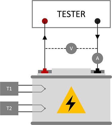
Although both sensors are located in two different places inside the battery, their measurements should not present great differences. This occurs due to the fact that lithium-ion cells have a homogeneous temperature distribution. Furthermore, for each measurement point |$T1$| and |$T2$|, two redundant sensors are placed to detect erroneous readings.
The present research deals with a battery LiFeBATT X-1P [2], composed of a LiFePO4 cell, whose nominal capacity is |$8 A\cdot h$|, with |$3.3 V$| of nominal voltage.
The four different stages of a capacity confirmation test detailed above are adapted to the LiFePO4 according to next steps.
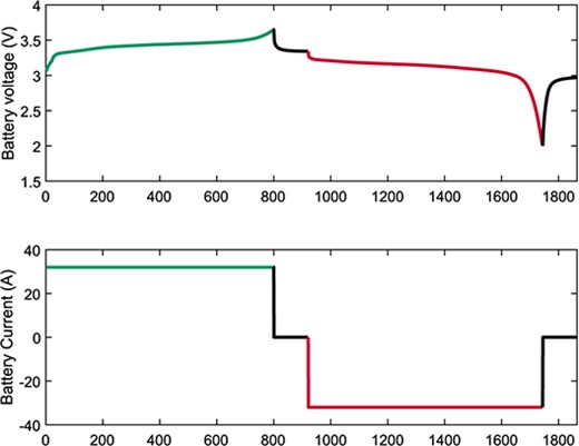
Charging phase. A constant current is send from the tester to the battery, resulting in a voltage rise from |$3 V$| up to |$3.65 V$|.
Resting phase with battery charged. The current flow stops at |$3.65 V$| and the voltage decreases to the nominal value of |$3.3 V$|.
Discharging phase. During this stage, a constant current is demanded by the tested until the voltage reaches |$2 V$|.
Resting phase with battery uncharged. Once the voltage is |$2 V$|, the current flow stops and, consequently, the voltage rises up to |$3 V$|. Hence, it can be repeated the process from Step 1.
The current and voltage measured during one test cycle is shown in Figure 2. When the current flows from the battery to the tester, it is considered negative and it is considered positive otherwise. The charge and discharge phases are represented with green and red traces, respectively, while the rest phases are represented with black traces
Voltage and current during one test cycle.
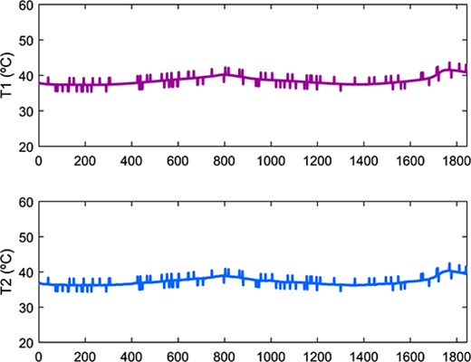
In addition to the current and voltage, the energy flow, in ampere-hour, can be monitored by integrating the current over time. The upper side of Figure 3 represents the energy balance at the battery during the capacity confirmation test, in terms of SOC (%) (%), with the same trace colour criteria as Figure 2. At the bottom of Figure 3, the evolution of temperature during one cycle is presented.
Energy and temperatures measured in one cycle.

2.3 Dataset and fault emulation
During the testing process described in the previous subsection, the state of the cell is assessed with a sample rate of 1 Hz. The variables registered are the current, the voltage, the SOC and the two temperatures measured by the sensors. As the test procedure consisted on 9 cycles, which are divided into four different steps, the total number of samples are the following.
Charging phase: 6610 samples.
Resting phase with battery charged: 967 samples.
Discharging phase: 6620 samples.
Resting phase with battery uncharged: 975 samples.
The real data registered correspond to a correct operation, and the objective of this work is to detect faults in the battery. Then, 25% of the dataset is randomly chosen to emulate the occurrence of anomalies. These instances were modified by changing the temperature measured a certain deviation, which, according to battery manufacturer, would represent the appearance of degradation. In this work, a comparative analysis of the capabilities of different one-class techniques is sought. Hence, the temperature deviation represented a 5%, 10%, 15% and 20% of the original measurement. Due to the fact that the two temperature sensors should have similar behaviour, the deviation is applied over both of them. Figure 4 represents an example of how fault situations are emulated during one test cycle by deviating a 5% of the correct measurement.
Temperature deviations during one test sample.
3 Methods
This section introduces the hybrid classifier approach proposed to detect anomalies during the capacity confirmation test. Furthermore, a brief explanation of each of the tested techniques is presented.
3.1 Classification approach
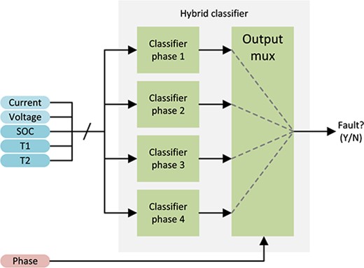
As stated in Subsection 2.2, the anomaly detection process must face the possibility of dealing with different operating points. Consequently, a hybrid classifier is implemented according to Figure 5.
Hybrid classifier approach.
The best classifier for each operating regime is chosen following the procedure shown in Figure 6. For a given phase |$p$|, each of the |$k$| methods detailed in next subsection are tested. Furthermore, different |$n$| hyperparameters are swept for each technique. Finally, the classifier with the best result is the one chosen for the hybrid topology.
Schematic process to obtain the best classifier for a phase |$p$|.
3.2 Anomaly detection techniques
The different techniques considered to implement the fault detection system are detailed in this subsection.
3.2.1 Gaussian classifier
The use of probability density functions can approximate the behaviour of the training set. A simple and direct way to apply this approach consists of using a Gaussian function to model the target class [10]. Then, once the Gaussian function is calculated, the criteria to determine the anomalous nature of a test sample are based on its probability density value.
This technique has been used in many different applications, giving especially successful results when the data are normally distributed [6]. Furthermore, its simplicity results in extremely low computation times, which is one of the main strengths of this method [29].
3.2.2 Parzen density estimation
This density estimation method aims to model the data by means of the use of non-parametric Parzen density estimator (PDE). In this case, a Gaussian kernel is combined with the covariance matrix over each target instance during the training process [17].
A key feature that is also shared with Gaussian model technique is that the behaviour of the achieved classifier has an extremely close relationship with the nature of the target set. Unsuccessful results should be achieved when the data size is not significantly great or the number of outliers in the training set is high [6].
3.2.3 Principal component analysis
The use of principal component analysis (PCA) has been commonly used for dimensional reduction tasks [31]. However, this technique can be configured as a one-class reconstruction method [21]. The main basis of this technique rests in the fact of finding the direction with greater data variability, known as components [31]. These vectors can be used to perform a linear projections of the original data over lower data dimensions.
Then, the criteria to determine the anomalous behaviour of a test sample is based on the reconstruction error. This is defined as the difference between the original point and the projected data. This approach makes the assumption that anomalies will result in high reconstruction error [29].
3.2.4 Minimum spanning trees
The main basis of minimum spanning trees (MSTs) is focused on obtaining a set of edges of an undirected connected graph with the lowest total weight [24]. This method, which has been applied initially to develop telecommunications and power grids, can also be considered for one-class classification tasks [29].
Once the tree is calculated using only data from the target set, the criteria to detect an anomalous test instance are based on the distance to the nearest edge. If this distance is higher than a given threshold, then the anomaly is detected [23].
3.2.5 Support vector data description
The support vector data description (SVDD) is a one-class technique classified as a boundary method. This technique has its origin in the commonly used support vector machine, which aims to project the data over a high-dimensional feature space. Then, a hyperplane is constructed looking for the maximum distance between the target set and the origin.
From this basic concept, SVDD performs a similar process. In this case, a hypersphere containing all training instances is implemented instead of an hyperplane [29]. The criteria to identify the anomaly occurrence are based on the membership of the test sample to the hypersphere [29].
4 Experiments to Validate the Proposal
Before the description of all experiments, it is important to remark that this research has two main objectives. First, a detailed analysis of the performance of five different one-class techniques is going to be performed. In addition to the hyperparameters influence of each technique, the influence of the fault nature will also be assessed. For this reason, the faults are generated using different percentage deviations. The second main objective is to achieve the best hybrid classifier. This means that, for each of the four operating points, the technique with the best performance is chosen to detect faults during the capacity confirmation test of a LiFePO4 battery.
From this goals, the experiments carried are the one summarized below.
The dataset is divided into four phases, as explained in Subsection 2.3 (Charging phase, resting phase with battery charged, discharging phase and resting phase with battery uncharged).
For the data belonging to each phase, four different outlier generation processes are tested: the temperature measurements are modified as 5%, 10%, 15% and 20%.
Hence, for each anomaly detection set, the five techniques detailed in the previous section are applied.
Finally, for each technique, several hyperparameters and data preprocessing are tested using a 10|$k$|-|$fold$| cross-validation. The different data conditioning tested are the following.
Data normalization using a 0 to 1 criteria. For each variable, the maximum registered is converted to 1 and the minimum to 0. The intermediate values are scaled accordingly.
Data normalization using the z-score criteria. This value measures, for each variable, the number of standard deviations that a value is away from the mean [27].
The data are not preprocessed and treated without conditioning.
The hyperparameter tested are summarized in Table 1.
Finally, the criteria to determine the best classifier configuration are based on the area under the receiving operating curve (AUC), which calculates a relationship between true positive rate and false positive rate. This indicator shows a representative value of the classifier behaviour, regardless the class distribution [5, 13].
Hyperparameters tested for each technique.
| Technique | Hyperparameter | Tested values |
|---|---|---|
| Gaussian model | Outliers fraction in the target set (|$\varTheta $|) | 0:5:20 |
| Regularization parameter (|$\beta $|) | 0:0.001:0.01 | |
| PDE | Outliers fraction in the target set (|$\varTheta $|) | 0:5:20 |
| Width parameter (|$\alpha $|) | 0:0.01:0.1 | |
| PCA | Outliers fraction in the target set (|$\varTheta $|) | 0:5:20 |
| Number of components (|$n_c$|) | 1:1:|$n_{var}$| | |
| MST | Outliers fraction in the target set (|$\varTheta $|) | 0:5:20 |
| SVDD | Outliers fraction in the target set (|$\varTheta $|) | 0:5:20 |
| Width of RBF kernel (|$\sigma $|) | 1:0.5:5 |
5 Results and Comparative Analysis
The best results obtained for each capacity confirmation test phase, anomaly generation method and technique are summarized in this section. In addition to the best AUC reached, the configured hyperparameters and preprocessing for these results are presented. ‘With the aim of giving a general idea of the throughput of each technique, the authors also present the computation time. However, this value might be subjected to the processor features and could not offer a direct idea of the technique performance. Then, for each test run, the highest computation time was assigned a 100 %, while the rest of times are proportionally graded. For example, if the slowest technique needs 10 seconds to train the classifier, this should present the 100%, and any technique with 5 seconds of training time should be graded with a 50% of computation effort.’
The results achieved for detecting anomalies during the charging process of the capacity confirmation test are shown in Table 2. The experiments carried out over the set comprised data from the resting phase with the battery charged, led to the results in Table 3. The performance of each one-class technique when detecting faults during the battery discharging phase are presented in Table 4. Finally, the best results for the resting phase with the battery discharged are shown in Table 5.
Best results for battery charging set.
| Deviation | Technique | AUC (%) | Preproc. | Configuration | Effort (%) | |
|---|---|---|---|---|---|---|
| 5% | Gauss | 100.000 | 0–1 | |$\beta $|=0.01 | |$\varTheta $|=0 | 0.006 |
| PDE | 85.485 | ZS | |$\alpha $|=0.05 | |$\varTheta $|=0 | 3.795 | |
| PCA | 99.990 | 0–1 | |$n_{c}$|=4 | |$\varTheta $|=0 | 0.026 | |
| MST | 99.990 | — | — | |$\varTheta $|=0 | 3.223 | |
| SVDD | 99.848 | ZS | |$\sigma $|=3.5 | |$\varTheta $|=0 | 100.000 | |
| 10% | Gauss | 100.000 | 0–1 | |$\beta $|=0.005 | |$\varTheta $|=0 | 0.008 |
| PDE | 89.717 | ZS | |$\alpha $|=0.05 | |$\varTheta $|=0 | 4.701 | |
| PCA | 99.990 | 0–1 | |$n_{c}$|=4 | |$\varTheta $|=0 | 0.045 | |
| MST | 99.990 | — | — | |$\varTheta $|=0 | 5.617 | |
| SVDD | 99.879 | ZS | |$\sigma $|=4 | |$\varTheta $|=0 | 100.000 | |
| 15% | Gauss | 99.990 | — | |$\beta $|=0 | |$\varTheta $|=0 | 0.056 |
| PDE | 91.646 | ZS | |$\alpha $|=0.1 | |$\varTheta $|=0 | 3.614 | |
| PCA | 99.990 | — | |$n_{c}$|=1 | |$\varTheta $|=0 | 0.074 | |
| MST | 100.000 | — | — | |$\varTheta $|=0 | 3.973 | |
| SVDD | 99.889 | ZS | |$\sigma $|=4 | |$\varTheta $|=0 | 100.000 | |
| 20% | Gauss | 100.000 | 0–1 | |$\beta $|=0.006 | |$\varTheta $|=0 | 0.003 |
| PDE | 92.990 | ZS | |$\alpha $|=0.03 | |$\varTheta $|=0 | 3.505 | |
| PCA | 99.990 | 0–1 | |$n_{c}$|=4 | |$\varTheta $|=0 | 0.031 | |
| MST | 100.000 | — | — | |$\varTheta $|=0 | 3.671 | |
| SVDD | 99.909 | ZS | |$\sigma $|=4.5 | |$\varTheta $|=0 | 100.000 |
Best results for resting with charged battery set.
| Deviation | Technique | AUC (%) | Preproc. | Configuration | Effort (%) | |
|---|---|---|---|---|---|---|
| 5% | Gauss | 99.931 | ZS | |$\beta $|=0.002 | |$\varTheta $|=0 | 1.875 |
| PDE | 90.833 | ZS | |$\alpha $|=0.03 | |$\varTheta $|=0 | 64.884 | |
| PCA | 99.931 | — | |$n_{c}$|=1 | |$\varTheta $|=0 | 64.884 | |
| MST | 99.931 | — | — | |$\varTheta $|=0 | 52.759 | |
| SVDD | 99.444 | ZS | |$\sigma $|=5 | |$\varTheta $|=0 | 100.000 | |
| 10% | Gauss | 99.931 | — | |$\beta $|=0.002 | |$\varTheta $|=0 | 2.521 |
| PDE | 91.944 | ZS | |$\alpha $|=0.04 | |$\varTheta $|=0 | 28.078 | |
| PCA | 99.861 | — | |$n_{c}$|=1 | |$\varTheta $|=0 | 36.734 | |
| MST | 99.931 | — | — | |$\varTheta $|=0 | 53.420 | |
| SVDD | 98.958 | ZS | |$\sigma $|=2 | |$\varTheta $|=0 | 100.000 | |
| 15% | Gauss | 99.931 | — | |$\beta $|=0.003 | |$\varTheta $|=0 | 2.802 |
| PDE | 91.389 | ZS | |$\alpha $|=0.02 | |$\varTheta $|=0 | 78.437 | |
| PCA | 99.931 | — | |$n_{c}$|=1 | |$\varTheta $|=0 | 10.167 | |
| MST | 99.931 | — | — | |$\varTheta $|=0 | 76.309 | |
| SVDD | 99.583 | ZS | |$\sigma $|=5 | |$\varTheta $|=0 | 100.000 | |
| 20% | Gauss | 99.931 | — | |$\beta $|=0.001 | |$\varTheta $|=0 | 1.732 |
| PDE | 92.014 | ZS | |$\alpha $|=0.03 | |$\varTheta $|=0 | 58.332 | |
| PCA | 99.861 | — | |$n_{c}$|=2 | |$\varTheta $|=0 | 10.145 | |
| MST | 99.931 | — | — | |$\varTheta $|=0 | 66.192 | |
| SVDD | 99.514 | ZS | |$\sigma $|=4 | |$\varTheta $|=0 | 100.000 |
Best results for battery discharging set.
| Deviation | Technique | AUC (%) | Preproc. | Configuration | Effort (%) | |
|---|---|---|---|---|---|---|
| 5% | Gauss | 99.990 | — | |$\beta $|=0 | |$\varTheta $|=0 | 1.875 |
| PDE | 92.893 | ZS | |$\alpha $|=0.01 | |$\varTheta $|=0 | 64.884 | |
| PCA | 99.990 | — | |$n_{c}$|=2 | |$\varTheta $|=0 | 64.884 | |
| MST | 99.990 | — | — | |$\varTheta $|=0 | 52.759 | |
| SVDD | 99.445 | ZS | |$\sigma $|=3 | |$\varTheta $|=0 | 100.000 | |
| 10% | Gauss | 99.990 | — | |$\beta $|=0 | |$\varTheta $|=0 | 2.521 |
| PDE | 91.058 | 0-1 | |$\alpha $|=0.04 | |$\varTheta $|=0 | 28.078 | |
| PCA | 99.990 | ZS | |$n_{c}$|=3 | |$\varTheta $|=0 | 36.734 | |
| MST | 100.000 | 0-1 | — | |$\varTheta $|=0 | 53.420 | |
| SVDD | 99.879 | ZS | |$\sigma $|=4 | |$\varTheta $|=0 | 100.000 | |
| 15% | Gauss | 99.990 | — | |$\beta $|=0 | |$\varTheta $|=0 | 2.802 |
| PDE | 93.438 | ZS | |$\alpha $|=0.03 | |$\varTheta $|=0 | 78.437 | |
| PCA | 99.990 | — | |$n_{c}$|=1 | |$\varTheta $|=0 | 10.167 | |
| MST | 100.000 | — | — | |$\varTheta $|=0 | 76.309 | |
| SVDD | 99.899 | ZS | |$\sigma $|=4 | |$\varTheta $|=0 | 100.000 | |
| 20% | Gauss | 99.990 | — | |$\beta $|=0.005 | |$\varTheta $|=0 | 1.732 |
| PDE | 95.151 | ZS | |$\alpha $|=0.01 | |$\varTheta $|=0 | 58.332 | |
| PCA | 99.990 | — | |$n_{c}$|=1 | |$\varTheta $|=0 | 10.145 | |
| MST | 100.000 | — | — | |$\varTheta $|=0 | 66.192 | |
| SVDD | 99.899 | ZS | |$\sigma $|=4 | |$\varTheta $|=0 | 100.000 |
Best results for resting with discharged battery set.
| Deviation | Technique | AUC (%) | Preproc. | Configuration | Effort (%) | |
|---|---|---|---|---|---|---|
| 5% | Gauss | 99.932 | — | |$\beta $|=0.001 | |$\varTheta $|=0 | 1.999 |
| PDE | 90.274 | ZS | |$\alpha $|=0.02 | |$\varTheta $|=0 | 33.822 | |
| PCA | 99.932 | 0–1 | |$n_{c}$|=2 | |$\varTheta $|=0 | 8.412 | |
| MST | 100.000 | — | — | |$\varTheta $|=0 | 30.397 | |
| SVDD | 99.396 | ZS | |$\sigma $|=5 | |$\varTheta $|=0 | 100.000 | |
| 10% | Gauss | 99.932 | — | |$\beta $|=0.005 | |$\varTheta $|=0 | 1.191 |
| PDE | 90.411 | ZS | |$\alpha $|=0.03 | |$\varTheta $|=10 | 33.844 | |
| PCA | 99.932 | — | |$n_{c}$|=1 | |$\varTheta $|=0 | 5.544 | |
| MST | 100.000 | — | — | |$\varTheta $|=0 | 33.294 | |
| SVDD | 99.247 | ZS | |$\sigma $|=3 | |$\varTheta $|=0 | 100.000 | |
| 15% | Gauss | 99.932 | — | |$\beta $|=0.005 | |$\varTheta $|=0 | 0.780 |
| PDE | 90.890 | ZS | |$\alpha $|=0.01 | |$\varTheta $|=10 | 24.987 | |
| PCA | 99.931 | — | |$n_{c}$|=2 | |$\varTheta $|=0 | 5.861 | |
| MST | 100.000 | ZS | — | |$\varTheta $|=0 | 36.924 | |
| SVDD | 99.589 | ZS | |$\sigma $|=5 | |$\varTheta $|=0 | 100.000 | |
| 20% | Gauss | 99.932 | — | |$\beta $|=0.001 | |$\varTheta $|=0 | 1.646 |
| PDE | 90.274 | ZS | |$\alpha $|=0.01 | |$\varTheta $|=0 | 43.535 | |
| PCA | 99.932 | — | |$n_{c}$|=2 | |$\varTheta $|=0 | 17.205 | |
| MST | 99.932 | — | — | |$\varTheta $|=0 | 36.570 | |
| SVDD | 99.315 | ZS | |$\sigma $|=5 | |$\varTheta $|=0 | 100.000 |
5.1 Comparative analysis
This subsection highlights the main features of each technique according to the results achieved and, consequently, determines the best hybrid classifier configuration.
5.1.1 One-class classifiers analysis
Gaussian model. The Gaussian one-class classifier presented a remarkable low computation effort. In all experiments, it is the one with the lowest computation time. In spite of its simplicity and speed, its performance is remarkable for all training sets, regardless the temperature deviation. On the other hand, the value of |$\varTheta $| is always 0, which means that the target set does not present a significant number of outliers. This feature is shared with the rest of techniques. Focusing on the parameter |$\beta $|, it does not follow a clear pattern, since its value varies from one experiment to another. Finally, the good results achieved using this technique indicates that the dataset may present a normal distribution.
Parzen Density Estimator Unlike Gaussian classifier, this method does not present an extremely good performance. Although the AUC values are the lowest and the computation effort is the second or third greatest, it is interesting to remark that it presents the trend of increasing performance when the temperature deviation increases. The optimum values of |$\alpha $| are also below 0.05, even though it was tested up to 0.1. Regarding the best preprocessing approach, this technique performs better with z-score normalization.
Principal component analysis The PCA classifiers has the second-lowest computation effort, which is a really interesting feature, especially, taking into consideration that the performance is among the three best for all sets. Focusing on the number of components, this value is not always the same and changes depending on the tested set. Regarding the data conditioning, training with raw data offer better results in all cases.
Minimum spanning tree The results obtained with this technique are always between the two best in all experiments, and they are achieved using raw data instead of data conditioning. Although this technique competes with Gaussian or PCA in terms of AUC, it is important to emphasize the significant computation effort, especially comparing it with those two techniques.
Support vector data description This last one-class technique has the main disadvantage of having a great computation effort, being the slowest method. When the dataset is greater (charging and discharging sets), it has a computation effort more than 30 times greater than the second-slowest method. In the rest of cases, the difference is not so remarked, although it is significant. This feature is especially negative when an online training process is implemented. Regarding the preprocessing stage, this technique performs better with z-score normalization, showing significant better results than the obtained with other conditioning. The width of RBF |$\sigma $| is not constant for all cases, varying from 2 to 5, depending on the set.
5.1.2 Hybrid one-class classifier
After the presented results and the detailed analysis of each classifier, the proposed fault detection system would have the following topology.
Charging phase.
– 5 % temperature deviation: Gaussian classifier with raw data, |$\beta $|=0 and |$\varTheta $|=0.
– 10 % temperature deviation: Gaussian classifier with 0-1 normalization, |$\beta $|=0.005 and |$\varTheta $|=0.
– 15 % temperature deviation: MST classifier with raw data and |$\varTheta $|=0.
– 20 % temperature deviation: Gaussian classifier with 0-1 normalization, |$\beta $|=0.006 and |$\varTheta $|=0.
Resting phase with battery charged.
– 5 % temperature deviation: Gaussian classifier with z-score normalization, |$\beta $|=0.002 and |$\varTheta $|=0.
– 10 % temperature deviation: Gaussian classifier with raw data, |$\beta $|=0.002 and |$\varTheta $|=0.
– 15 % temperature deviation: Gaussian classifier with raw data, |$\beta $|=0 and |$\varTheta $|=0.
– 20 % temperature deviation: Gaussian classifier with raw data, |$\beta $|=0.001 and |$\varTheta $|=0.
Discharging phase.
– 5 % temperature deviation: Gaussian classifier with raw data, |$\beta $|=0 and |$\varTheta $|=0.
– 10 % temperature deviation: MST classifier with 0-1 normalization and |$\varTheta $|=0.
– 15 % temperature deviation: MST classifier with raw data and |$\varTheta $|=0.
– 20 % temperature deviation: MST classifier with raw data and |$\varTheta $|=0.
Resting phase with battery uncharged.
– 5 % temperature deviation: MST classifier with raw data and |$\varTheta $|=0.
– 10 % temperature deviation: MST classifier with raw data and |$\varTheta $|=0.
– 15 % temperature deviation: MST classifier with z-score normalization and |$\varTheta $|=0.
– 20 % temperature deviation: Gaussian classifier with raw data, |$\beta $|=0.001 and |$\varTheta $|=0.
It can be derived from these results that, for each operating point of the battery, four different classifiers are taken into account. However, if a classifier performs well with 5% of temperature deviation, it does not mean that it detects properly the 20% deviations. The best way to face this problem is to use an or logic gate. Hence, for a given operating point, the fault is detected if at least one of the four classifiers indicate it.
6 Conclusions and Future Works
The present work deals with the fault detection in a capacity confirmation test performed over a LiFePO4 battery. Five different one-class techniques are proposed to implement a hybrid intelligent system capable of detecting slight deviation in the battery temperature. This tool could represent a really important breakthrough since it can help the manufacturer to identify the early deterioration in a battery. The contribution of this paper is especially important, taking into consideration the great potential of this kind of batteries in an immediate future.
The increasing interest of one-class classification techniques to solve fault detection problems emphasizes the importance of the present work. A detailed analysis of each one is carried out, remarking the main strengths and weaknesses of each one. Gaussian classifier has shown really good results with very low computation effort. However, this fact can be the result of normally distributed data, so this method could lead worse results with high non-linear data. The MST performed almost as good as Gaussian, although it implies a significantly greater training times. Focusing on improving the computation effort with good results, PCA has a remarkable performance. The SVDD classifiers present the main disadvantage of high computation cost, while PDE offered the worst results in all experiments.
The main idea of studying the computation effort is related to the possibility of establishing an edge computing topology, where the fault detection is implemented in a decentralized environment. This innovative idea is suitable not only for fast techniques like PCA or Gauss but also for more computationally expensive techniques since processors are dedicated to specific tasks.
In addition, due to the difficulty of obtaining real anomalies, a fault generation method is developed to check the behaviour of the classifiers. This method could be applied to a wide range of cases, such as the alteration in sensors or actuators operation.
Although the anomaly generation is suitable for the case of study, in future works, the implementation of different methods to obtain a dataset of faults could be interesting. Instead of percentage, different criteria, such as standard deviation, variance or even a time series approach, would present a useful tool to check classifiers performance [20].
This work addresses the problem of battery degradation. However, it could be possible that the fault is detected due to a measurement error. Then, developing imputation techniques or intelligent models to replace the wrong measurement would allow to dispense with recurrent sensors and recover the missing data [19].
The proposed hybrid topology divides the dataset into four groups, depending on the phase of the capacity confirmation test. Further works could consider the possibility of applying clustering techniques over each set, to divide the data into different subgroups. In addition to clustering, the application one-class techniques based on random projections, such as NCBoP or APE [22], could help to achieve interesting results, especially if the data are well separated.
Finally, the proposed method could be improved in future works by retraining the system after a certain time. This would be interesting, since the battery can evolve due to its use, so the new data should be taken into consideration to implement the classifier.
Conflict of interest
The authors declare no conflict of interest.
References
