


Abstract
We developed mathematical models to analyze a large dengue virus (DENV) epidemic in Reunion Island in 2018–2019. Our models captured major drivers of uncertainty including the complex relationship between climate and DENV transmission, temperature trends, and underreporting. Early assessment correctly concluded that persistence of DENV transmission during the austral winter 2018 was likely and that the second epidemic wave would be larger than the first one. From November 2018, the detection probability was estimated at 10%–20% and, for this range of values, our projections were found to be remarkably accurate. Overall, we estimated that 8% and 18% of the population were infected during the first and second wave, respectively. Out of the 3 models considered, the best-fitting one was calibrated to laboratory entomological data, and accounted for temperature but not precipitation. This study showcases the contribution of modeling to strengthen risk assessments and planning of national and local authorities.
(See the Editorial Commentary by Colston on pages 1–3.)
The course of an epidemic depends on the level of immunity in the population and the underlying transmissibility of the pathogen. Often the latter is assumed constant. However, for arboviruses, this seems an oversimplistic assumption because transmissibility is strongly affected by climate [1–4]. It is therefore important to determine how inclusion of this understanding in mathematical models may improve their ability to reproduce arbovirus epidemic dynamics.
Consider dengue as an example. Different approaches have been proposed to assess the association between climate and dengue transmission: Lambrechts et al [2] and Mordecai et al [3] used laboratory entomological data while Perkins et al [4] relied on epidemiological case data. Each of these approaches provides somewhat different characterizations of the association between climatic variables and dengue transmissibility.
Here, we evaluate the forecasting performance of these different models describing the impact of climate on time-varying transmissibility of dengue virus (DENV), in the context of a large epidemic in Reunion Island, an overseas department of France in the Indian Ocean. For 40 years prior to this outbreak, DENV circulation had only been sporadic in the island despite the perennial presence of Aedes albopictus [5, 6]. Reunion Island experienced only 1 large DENV epidemic (serotype 2) in 1977–1978 [7, 8], as well as a large chikungunya virus (CHIKV) outbreak in 2005–2006 [9]. Both epidemics infected about a third of the population and demonstrated that large self-sustained arbovirus outbreaks were indeed possible. An important surge of dengue cases in early 2018 quickly became a cause for concern for local authorities given their past experience with CHIKV and DENV. To strengthen their risk assessment, epidemiologists at Santé Publique France and its regional office in Reunion Island requested modelling support from Institut Pasteur to obtain quantitative estimates of risk and assess uncertainties along the unfolding of the epidemic. This work provides a valuable test bed to assess (1) how generalizable the association climate-DENV transmission is, and (2) whether this knowledge can effectively be used to inform planning in newly affected locations.
METHODS
Epidemiological Data
Our models were fitted to weekly counts of confirmed cases recorded from epidemiological and laboratory surveillance on the island. The surveillance is based on the active participation of hospitals and general practitioners as well as public and private biological laboratories that report DENV infections. A confirmed case was defined as a patient with a positive reverse transcription polymerase chain reaction (RT-PCR) or seroconversion (4-fold increase in immunoglobulin G [IgG] titer between 2 samples taken 2 weeks apart). Because it took about 1 week to consolidate the data, when recalibrating our models, we only included data up to 2 weeks before the date of the analysis. The complete dataset is provided as a single CSV file (Supplementary Material).
Serological Data
The seroprevalence of DENV among blood donors in Reunion Island was estimated at 3.1% (95% confidence interval [CI], 2.2%–3.9%) in 2008 [10], and only a few hundred dengue fever cases were reported between 2008 and 2018 [11, 12]. For our first assessments, we therefore assumed that 100% of the population was susceptible to DENV at the beginning of 2018. However, this assumption changed in May 2019 when new serological data from studies performed by the French blood bank (Établissement Français du Sang) using samples collected in August 2013 became available. These studies estimated the seroprevalence among blood donors at 24.1% in 2013 (Gallian and de Lamballerie, personal communication). Considering that individuals younger than 18 years old are not included in these surveys and that 5 years had passed since 2013, we then assumed that the proportion of the population susceptible to DENV on 1 January 2018 was 85% (Supplementary Material 1).
Mathematical Model
To characterize the dengue epidemic trajectory, we developed an SIR (susceptible-infectious-recovered) model in which the transmission rate β(t) varies with time according to:
where β0 is a constant to be estimated and s(T(t), P(t)) is a scaling factor that depends on temperature (T) and precipitation (P). Because there is still substantial uncertainty about the best way to model how the transmission of DENV (and other arboviruses) is influenced by climate conditions [1–4], we used 3 models for s(T(t), P(t)):
The first, by Lambrechts et al [2], was calibrated using laboratory entomological data describing how the probability of DENV transmission for Aedes aegypti mosquitoes varies with the temperature and daily temperature fluctuations.
The second, by Mordecai et al [3], was calibrated using a large amount of laboratory entomological data on Ae. aegypti and Ae. albopictus describing the effect of temperature on the mosquito lifecycle and the probability of transmission for dengue, chikungunya, and Zika viruses.
The third, by Perkins et al [4], was calibrated using epidemiological case data collected during chikungunya outbreaks in the Americas.
All 3 models capture the effect of temperature; the model by Perkins et al is the only one to also account for precipitation (see Supplementary Material 3 for more details).
We model the number of incident cases assuming a Poisson observation process. The likelihood of observing incident cases on week given the expected number of infections for that week is given by the density of a Poisson distribution:
where ρ is the detection probability.
The number of infectious individuals at the start of the epidemic (ie, in January 2018) and at the beginning of the second wave (ie, start of November 2018) were considered as free parameters.
In Supplementary Material 2 we present 5 variants of the model described above based on the SEIR (susceptible-exposed-infectious-recovered) model, that is, with different assumptions about the incubation and infectious periods (see also discussion in Supplementary Material 5).
DENV Natural History
The generation time for DENV (defined as the average time interval between consecutive infections) has been estimated to be between 2 and 3 weeks [13, 14]. We therefore considered 2 scenarios where the generation time was 15 and 21 days, respectively.
Detection Probability
The detection probability corresponds to the probability that a person infected with dengue is detected by the surveillance system. It is the product of the proportion of infections that are symptomatic and of the proportion of symptomatic infections that consult a doctor and get tested. The proportion of infections that result in symptoms is poorly understood and depends on a number of factors, including host population genetics, the serotype as well as the genotype of the infecting virus, and the immune history of the population. Rather than using a single value, we have therefore conservatively used the range between 20% and 50% [15]. Based on local expert opinion, we assumed that between 50% and 80% of infected symptomatic individuals consult their doctor and have a sample collected for laboratory confirmation. Under these assumptions, we expect that the detection probability should lie between 10% and 40%; however, it is not possible to estimate this parameter early on in the epidemic from case data only. To assess the impact of this parameter on our forecasts, we ran our model for fixed values of the detection probability between 10% and 40% and present scenarios where this probability is fixed to 10% and 40%. We also investigated how estimates of this quantity evolve as data accumulate.
Climatic Scenarios
To compute the scaling factors s(T(t), P(t)) at each time point, we relied on sinusoidal fits of daily temperature and precipitation data provided by Météo France and spanning the time period from 2004 to 2019 (Supplementary Material 4 and Supplementary Figure 5). To account for uncertainty in climate variables for dates following the time point at which the analyses were performed, we considered 3 different scenarios:
average temperature scenario: average temperatures and precipitations calculated from the available data;
cold temperature scenario: average temperatures calculated from the coolest year (ie, lowest yearly average temperature) in the dataset (2005); no difference in terms of precipitation;
warm temperature scenario: average temperatures calculated from the warmest year (ie, highest yearly average temperature) in the dataset (2015); no difference in terms of precipitation.
Estimation and Model Comparison
Parameters were estimated via Markov Chain Monte Carlo (MCMC) sampling with uniform noninformative priors. We used the deviance information criterion (DIC) for model comparison. Smaller DIC values indicate better adequacy to the data. Differences of DIC above 4 were considered substantial. The model was implemented in C++ and is available, together with the epidemiological and climate data used for the analyses, on GitHub. We assumed all model parameters were constant for the duration of the epidemic.
RESULTS
From the start of the epidemic in January 2018 to 10 December 2019, more than 24 800 confirmed cases were notified (Figure 1A); 2405 cases presented to an emergency department, 732 cases were hospitalized, with 20 deaths—12 of which directly related to dengue [16]. Figure 1B and 1C show seasonal variations in temperature and precipitation.
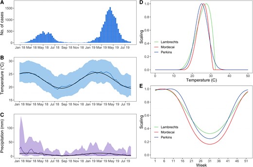
Epidemic curve, climate, and scaling factors modulating the transmission rate in the SIR (susceptible-infectious-recovered) model. A, Epidemic curve. The bars represent the weekly number of confirmed cases. B, Temperature in degrees Celsius and (C) precipitation in mm. The climate model fitted to the last 15 years of data is represented by the black line while measurements during the study period are represented in color (colored lines represent the averages while the colored areas encompass the 2.5 and 97.5 percentiles). D, Scaling factor versus temperature. E, Scaling factor versus time for a typical year in Reunion Island.
Figure 1D shows that, from a theoretical perspective, the temperature at which transmission peaks and the seasonality of DENV transmission in Reunion Island change slightly whether we consider the model of Lambrecht [2], Mordecai [3], or Perkins [4]. In particular, the model by Lambrechts et al shows a less pronounced reduction of transmission during the austral winter months than the other 2 models (Figure 1E).
First Assessment in July 2018
Our first assessment was performed in July 2018. At that time, the main concern was the possible persistence of DENV transmission during the austral winter 2018. Figure 2 shows the epidemic trajectories anticipated by the different models in July 2018 and up to January 2020. Our main conclusions at the time were that (1) uncertainties about the future course of the epidemic remained important; but (2) despite the substantial heterogeneities observed between models, all of them forecasted that a second epidemic wave would occur; and (3) in most scenarios (11 of 12 scenarios), the second wave was forecasted to be larger than the first one. This pattern closely resembled the 2-wave chikungunya epidemic that hit Reunion Island in 2005–2006 [9] and indicated that persistence of DENV transmission during the austral winter 2018 was a likely scenario.
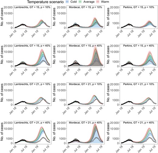
Epidemic forecasts up to January 2020 from data available in July 2018 for different model variants. In each panel is indicated the combination of model (Lambrechts, Mordecai, or Perkins), generation time (GT = 21 or 15 days), and detection probability (ρ = 10% or 40%). Black circles represent data points used for model calibration while white circles represent future data points (not used for model calibration). Forecasts from the models are represented in color for different temperature scenarios. To improve the figure readability the y-axis of all panels is on a square root scale.
Model Comparison
While most models had similar statistical support at the beginning of the epidemic, as more data became available, the Lambrechts model with a generation time (GT) = 15 days had consistently lower DIC than other models (Figure 3A); that is, it provided a better fit to the data already observed. Early in the epidemic, there was not sufficient information in the data to estimate the detection probability ρ (Figure 3B), and we therefore presented forecasts for ρ contained within its expected range, 10%–40%. However, from about the start of the second wave (November 2018), scenarios with a detection probability around 10%–20% received stronger statistical support so that we started to put more emphasis on forecasts associated with these values.
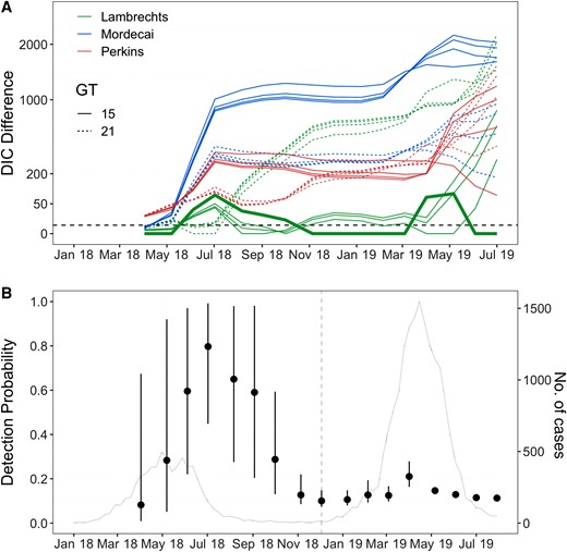
Model comparison and detection probability estimated with data available at different times during the epidemic. A, Deviance information criterion (DIC) difference with respect to the best fitting model. Solid lines indicate models with generation time (GT) = 15 days, while dashed lines indicate models with GT = 21 days. The 4 curves for each color and generation time combination correspond to detection probabilities ρ = 10%, 20%, 30%, and 40%. The dashed black line represents a DIC difference of 4, indicative of substantial model improvement. The thicker green line represents the best fitting model (Lambrechts, GT = 15 days, detection probability ρ = 10%). B, Detection probability estimated with data available at different times during the epidemic. The estimates were obtained by fitting the model by Lambrechts et al with GT = 15 days. Dots represent posterior means while the bars represent 95% credible intervals. The vertical dashed line in grey marks the switch to a model with an additional parameter (the proportion of infectious individuals at the beginning of the second epidemic wave). The grey line represents the epidemic curve.
Forecasts Over the Course of the Epidemic
Figure 4A–C shows the forecasts of all models (Lambrechts, Mordecai, or Perkins model; GT = 15 or 21 days; cold, average, or warm temperature scenario) for a detection probability ρ of 10% and 40%, and with respect to 3 key metrics: the total number of cases observed since the beginning of the epidemic (Figure 4A); the number of cases at the second peak (Figure 4B); and the timing of the second peak (Figure 4C). Figure 4D–F shows the same metrics but restricted to the model that performed best overall (ie, Lambrechts model with GT = 15 days).
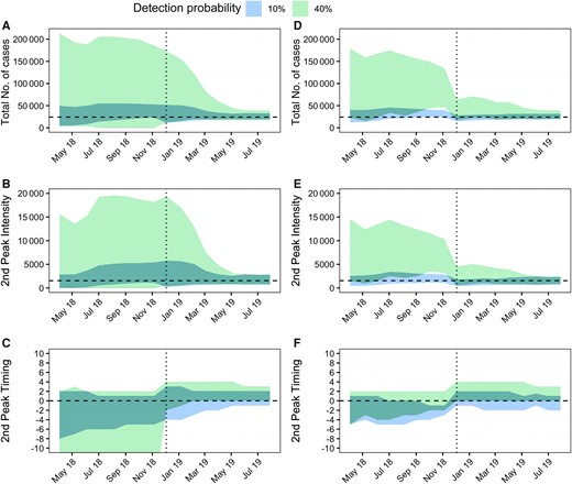
Forecasting performance during the epidemic. A and D, Total number of observed cases. B and E, Intensity of the second peak (ie, number of incident cases at the second epidemic peak). C and F, Error on the timing of the second peak (in weeks), calculated as the difference in weeks between forecasted and observed values. The colored areas represent the 95% forecast intervals for simulations obtained by (A–C) combining all models and all temperature scenarios and (D–F) the best performing model (Lambrechts with GT = 15 days) for all temperature scenarios. Blue indicates a detection probability of 10%, while green a detection probability of 40%. A, B, D, and E, The horizontal dashed line represents values observed during the epidemic. C and F, The horizontal dashed line represents a delay of zero weeks. A–F, The vertical dotted line marks the switch to models with an additional parameter (the proportion of infectious individuals at the beginning of the second epidemic wave).
We note that the most important sensitivity in forecasted metrics was driven by uncertainty about the detection probability. The forecasted total number of cases (Figure 4A and 4D) and size of the second peak (Figure 4B and 4E) were indeed much larger and with wider forecasted ranges when the detection probability was assumed to be 40% than when it was 10%; the forecasted range for the timing of the second peak was also substantially wider for ρ = 40% (Figure 4C and 4F). Throughout the epidemic, forecasts performed under the scenario of a detection probability of ρ = 10% have been remarkably accurate. As indicated earlier (Figure 3B), from November to December 2018, we started to get a strong signal from the data that the detection probability was in the lower range of values we considered (10%–20%). Although varying during the course of the epidemic, the cold temperature scenario was the temperature scenario that most consistently yielded the most accurate projections (10 out of 18 times).
By comparing Figure 4D–F to Figure 4A–C, we note a further gain in the quality of forecasts when relying on the best performing model (Lambrechts with GT = 15 days), although the gain is less than that obtained by selecting the correct detection probability. This model—with a detection probability of 10%—correctly forecasted both the total number of detected cases and the second peak intensity starting from April 2018 (Figure 4D and 4E). It also accurately forecasted the timing of the second peak from December 2018 onward (more than 4 months in advance), while having forecasted it on average 2 weeks earlier until then (Figure 4F).
Inferred Attack Rates and Immunity in the Population
Using data available as of August 2019, our best fitting model (Lambrechts with GT = 15 days) estimates a detection probability ρ = 11% (credible interval [CrI], 10%–12%). This estimate is largely insensitive to assumptions about the generation time (Supplementary Figure 1). Figure 5 shows the immunity against DENV2 in the population of Reunion Island as reconstructed by this model. We estimate that 26% (CrI, 21%–33%) of the population was infected during 1 of the 2 waves (8% and 18% in the first and second waves, respectively), which is roughly similar to the 35% attack rate estimated for the chikungunya epidemic in 2005–2006 [9]. Assuming that it takes 2 weeks for infected individuals to seroconvert, our results are in good agreement with seroprevalence estimates from 2 independent serological studies among blood donors (Gallian and de Lamballerie, personal communication) performed in April and October 2018 (Figure 5). Finally, our model estimates that the level of immunity against DENV2 after the 2 epidemic waves—and accounting for the initial level of immunity—was 41% (CrI, 36%–48%).
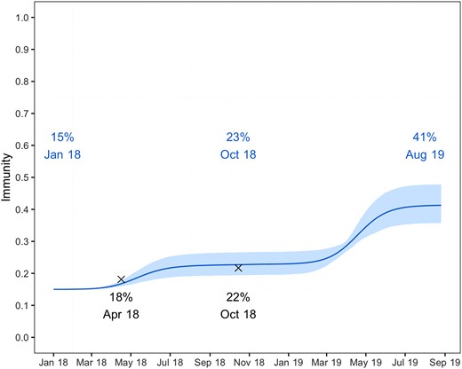
Level of immunity forecasted against dengue virus 2 in the population of Reunion Island. The solid line corresponds to the posterior mean, while the 95% credible interval is indicated as a colored area. Independent results from 2 serological surveys among blood donors performed during April and October 2018 are shown as black crosses.
DISCUSSION
We compared 3 mathematical models to forecast the DENV epidemic in Reunion Island in 2018–2019 and strengthen the risk assessments of Santé Publique France. Our forecasts accurately anticipated the observed epidemic trajectory and were used at a national and local level to inform planning and optimize resource allocation.
Epidemic forecasting in a context of emergence or reemergence is a difficult task because there is no historical record from the affected location that can be used to train predictive models. Here, we hypothesized that epidemiological and experimental data characterizing the association between climate and DENV transmission outside Reunion Island could provide key insights on DENV epidemic dynamics in the island. Our model captured existing uncertainties about key drivers and parameters. In particular, different models were considered to investigate how assumptions about the association between climate and DENV transmission (3 models), the generation time of dengue (2 models), temperature trends (3 models), and the detection probability could impact our forecasts. In Supplementary Figure 6 we show that a model ignoring climate or considering a simple modulation of the transmission rate following temperature trends would not have been able to capture the epidemic dynamics.
Forecasts were particularly sensitive to the assumption about the detection probability of incident infections. From November to December 2018, our analyses indicated that about 10%–20% of dengue infections were detected by the surveillance system. For that range of values, forecasts for the total number of cases, the size, and timing of the second peak were remarkably accurate throughout the epidemic. The fact that we started to be able to estimate the detection probability around the beginning of the second wave is consistent with theory that early in an epidemic, the exponential growth rate estimate, which summarizes information about the transmission potential, is independent of the detection probability. These expectations are confirmed in Supplementary Figure 7, which shows the posterior distributions of the detection probability and the mean generation time obtained with data available at different times of the epidemic: the detection probability can only be estimated once we are quite advanced in the second wave, while the generation time is only available at the end of the first wave. While it is interesting to retrospectively ascertain when the estimation of these quantities became possible, trying to estimate them from the limited data we had at the start of the epidemic to inform projections was doomed to fail. Instead, we decided to explore the performance of a well-defined set of models informed by prior knowledge on dengue (GT = 15 or 21 days, detection probability = 10%–40%). In such a context of limited data, we believe this approach is preferable to integration over vague priors, as it improves communication to policy makers, who can more easily understand sensitivity of projections to model parameters. At a more advanced stage of the epidemic, it is interesting to also explore the posterior distribution of model parameters and the associated projections (Figure 3B and Supplementary Figures 7 and 8). However, given that posterior estimates can be unstable (Figure 3B and Supplementary Figure 7), we believe it remains important to consider a broader range of parameter values than the one in the posterior distribution.
Given the sensitivity of forecasts to the detection probability, obtaining estimates of this parameter from independent data such as serosurveys in blood donors would have been extremely helpful to reduce uncertainties and strengthen confidence in our forecasts. This is a point we raised throughout the epidemic, highlighting how modelling can be used to identify complementary studies that are essential to reduce key knowledge gaps. In some cases, the detection probability may exhibit important variations during the time course of an epidemic, because of the evolution of testing protocols or of health care-seeking behaviors [17] and it is important to be able to track these changes through time with regular serosurveys. In the absence of such data, we made here the simplifying assumption that the detection probability was constant over time. In a sensitivity analysis (Supplementary Figure 4), we show that assuming a 3-fold increase in the detection probability at the start of the second epidemic wave would not impact the quality of our predictions for the epidemic curve of confirmed cases but would lower the estimated level of immunity in the population at the end of the second epidemic wave (32% vs 41%).
These 3 models were generated using different data sets, including epidemiological and laboratory experiments. The original intended purpose of these models was not necessarily to forecast epidemiological dynamics, as we have used them for here. For example, despite being the best fitting model, the Lambrechts model only focuses on differences in dissemination of the virus during midgut infection as a function of temperature and does not directly explore differences in mosquito density. However, mosquito densities also change with temperature and, in practice, we observe that this formulation also captures some of these differences. Similarly, the Lambrechts model was generated using Ae. aegypti data, rather than Ae. albopictus, the primary driver of transmission in Reunion Island. Consistent relationships between temperature and transmission potential have been observed for Ae. aegypti and Ae. albopictus, which may help explain this performance [18]. This highlights the relevance of laboratory-generated data in applications to the field, despite clear differences in conditions (eg, constant temperature and the use of laboratory-reared mosquitoes). Given the complexity of the association between climate and dengue transmission, we should not overinterpret results of this model comparison exercise. The relative performance of the different models may differ in different settings and it will therefore remain important to compare their performance in outbreaks in other locations.
In our models, we considered 3 climate trajectories (warm, cold, and average) for temperature and precipitation. However, such an approach imperfectly captures interannual variability, which may potentially reduce model predictive power. We found that temperatures measured during the epidemic period were close to expected temperatures (Figure 1B), but there were more discrepancies between observed and expected precipitations (Figure 1C). This may have affected the predictive power of the Perkins model that uses precipitations. More generally, this suggests that it may be difficult to correctly capture and predict precipitation dynamics, which may affect the performance of models that utilize this indicator.
Our analysis evaluated the predictive performance of 3 models characterizing the association between climate and dengue transmission, which is an important step to ascertain the relevance of these models. However, more research is needed to understand this association and improve forecasts of dengue risk. For example, in the context of Reunion, models describing the spatiotemporal distribution of mosquito populations may help produce maps of dengue risk [19], while the integration of climate change forecasts into these models is necessary to anticipate its impact both on mosquito populations and dengue risks [20].
This study showcases the contribution of modeling to strengthen the risk assessments of national and local authorities and to provide quantitative support to inform planning and resource allocation, especially for scaling the reinforcement of vector-control activities and the implementation of a rapid diagnostic test strategy.
Supplementary Data
Supplementary materials are available at The Journal of Infectious Diseases online (http://jid.oxfordjournals.org/). Supplementary materials consist of data provided by the author that are published to benefit the reader. The posted materials are not copyedited. The contents of all supplementary data are the sole responsibility of the authors. Questions or messages regarding errors should be addressed to the author.
Notes
Financial support. This work was supported by the ANR Investissement d’Avenir program, the Laboratoire d’Excellence Integrative Biology of Emerging Infectious Diseases program (grant number ANR-10-LABX-62-IBEID); the ANR INCEPTION project (grant number PIA/ANR-16-CONV-0005); and the European Union Horizon 2020 Program through the ZIK Alliance (grant number 734548). Funding to pay the Open Access publication charges for this article was provided by Institut Pasteur.
References
Author notes
Potential conflicts of interest. All authors: No reported conflicts. All authors have submitted the ICMJE Form for Disclosure of Potential Conflicts of Interest. Conflicts that the editors consider relevant to the content of the manuscript have been disclosed.

