


Abstract
Understanding how environmental variation influences population genetic structure can help predict how environmental change influences population connectivity, genetic diversity, and evolutionary potential. We used riverscape genomics modeling to investigate how climatic and habitat variables relate to patterns of genetic variation in 2 stonefly species, one from mainstem river habitats (Sweltsa coloradensis) and one from tributaries (Sweltsa fidelis) in 40 sites in northwest Montana, USA. We produced a draft genome assembly for S. coloradensis (N50 = 0.251 Mbp, BUSCO > 95% using “insecta_ob9” reference genes). We genotyped 1930 SNPs in 372 individuals for S. coloradensis and 520 SNPs in 153 individuals for S. fidelis. We found higher genetic diversity for S. coloradensis compared to S. fidelis, but nearly identical genetic differentiation among sites within each species (both had global loci median FST = 0.000), despite differences in stream network location. For landscape genomics and testing for selection, we produced a less stringently filtered data set (3454 and 1070 SNPs for S. coloradensis and S. fidelis, respectively). Environmental variables (mean summer precipitation, slope, aspect, mean June stream temperature, land cover type) were correlated with 19 putative adaptive loci for S. coloradensis, but there was only one putative adaptive locus for S. fidelis (correlated with aspect). Interestingly, we also detected potential hybridization between multiple Sweltsa species which has never been previously detected. Studies like ours, that test for adaptive variation in multiple related species are needed to help assess landscape connectivity and the vulnerability of populations and communities to environmental change.
Understanding aquatic landscape connectivity is crucial for assessing the vulnerability of species to environmental change (Mönkkönen and Reunanen 1999; Grummer et al. 2019; Liu et al. 2021) because landscape connectivity and structure can influence the adaptive potential of populations and communities via neutral and adaptive gene flow and other mechanisms (Balkenhol et al. 2017). River networks, with their hierarchical network structure and unidirectional flow, present challenges for understanding the patterns and drivers of population connectivity (Altermatt 2013; Tonkin et al. 2018).
The dendritic network structure of streams and rivers can strongly influence dispersal, gene flow, diversity, metapopulation dynamics, and landscape connectivity of aquatic organisms (Fagan 2002; Grant et al. 2007; Morrissey and De Kerckhove 2009; Brown and Swan 2010; Finn et al. 2011; Altermatt 2013; Fronhofer and Altermatt 2017; Tonkin et al. 2018). In rivers, metacommunity theory has been used to integrate local (e.g., environmental constraints) and regional (e.g., dispersal) effects, accounting for how influences at varying scales may affect local communities and populations (Loreau 2000; Shurin and Allen 2001; Urban 2004). Although dispersal is a fundamental process influencing gene flow in aquatic systems, it can be a weaker structuring force in headwaters (because of stronger influences of local environmental factors) compared to mainstem habitats (Brown and Swan 2010), especially for species without upstream migration patterns.
In river networks, genetic diversity often increases downstream for both aquatic and terrestrial organisms due to downstream-biased gene flow (Hänfling and Weetman 2006; Kikuchi et al. 2009; Alp et al. 2012; Torterotot et al. 2014; Paz-Vinas et al. 2015). However, at the landscape scale, small headwater streams are very abundant and can play a disproportionately important role in enhancing diversity because they are spatially isolated, differing more strongly in genetic and species composition (Myers et al. 2001; Wishart and Hughes 2003; Finn and Poff 2005, 2011; Hughes et al. 2009; Brown and Swan 2010; Finn et al. 2011). Though the interaction of spatial isolation and asymmetric gene flow has been found to maintain higher landscape genetic diversity across space (Morrissey and De Kerckhove 2009), it is not clear if this is the case for all aquatic macroinvertebrates (e.g., for pleurocerids, Redak et al. 2021). In addition to asymmetric gene flow, variation in habitat availability and declining genetic diversity along colonization routes can also change the balance between forces influencing diversity (dispersal patterns, drift, selection), resulting in downstream increases in genetic diversity (Paz-Vinas et al. 2015).
The degree of genetic differentiation between populations depends substantially on the dispersal ability of the organisms and their ability to persist in different portions of the network (Fisher 1997; Hughes et al. 1999; Wilcock et al. 2001; Alp et al. 2012). For organisms or life stages restricted to stream channels, the distance along streams generally predicts population differentiation better than direct distance between streams (Roberts et al. 2013), though more nuanced distance measures can be used (Tonkin et al. 2018). When organisms have a terrestrial adult stage that allows flight between streams more pathways for connectivity exist (Alp et al. 2012; Hughes et al. 1999; Macneale et al. 2005).
Most aquatic insects disperse along waterways (by drifting downstream as nymphs and/or through terrestrial flights as adults) and gene flow is strongly influenced by spatial isolation (Hynes 1970; Williams and Hynes 1976; Müller and Url 1982; Minshall and Petersen 1985; Mackay 1992; Palmer et al. 1996; Elliott 2003; Hughes et al. 2009). Many direct measurements (e.g., mark-recapture techniques) of aquatic insect dispersal within and along streams have been made (Williams and Hynes 1976; Benson and Pearson 1987; Freilich 1991; Hershey et al. 1993; Williams and Williams 1993; Kuusela and Huusko 1996; Winterbourn and Crowe 2001). However, dispersal of aquatic insects between streams or watersheds (laterally) is less common. Only small numbers of adult caddisflies (Order:Trichoptera) and stoneflies (Order: Plecoptera) have been detected moving away from the stream using direct measurements (Jackson and Resh 1989; Kovats et al. 1996; Collier and Smith 1998; Griffith et al. 1998; Briers et al. 2004; Macneale et al. 2005). Population genetic studies are more commonly used to assess the extent and potential mechanisms of aquatic insect dispersal at greater distances (Sweeney et al. 1986; Jackson and Resh 1992; Schmidt et al. 1995; Hughes et al. 1995, 1996; Bilton et al. 2001) due to the difficultly of detecting few individuals at greater distances (i.e., between watersheds). Some genetic studies suggest that lateral dispersal between watersheds (over land) may be more frequent than direct measurements indicate (Schmidt et al. 1995; Bunn and Hughes 1997; Kelly et al. 2001).
Few genetic studies of stream insects have used a study design that allows testing genetic differentiation within and between streams (but see Bilton et al. 2001) and few empirical studies have sampled multiple network locations (i.e., multiple locations on headwaters, intermediate branches, mainstem; Morrissey and De Kerckhove 2009; Altermatt 2013). Inferences have also been limited by available technology. Recent advances in genomic techniques, the availability of reference genome sequence assemblies, and thousands of DNA markers now allow more powerful genome-wide assessments of genetic differentiation in natural populations (Hendricks et al. 2018). Reference genomes are important because they allow discovery of more loci and higher-quality loci (i.e., removal of paralogs; Hand et al. 2015; Shafer et al. 2017).
Landscape genomics in aquatic systems (sometimes called riverscape genomics) investigates how population genetic differentiation may be influenced by different environmental factors (e.g., streamflow and water temperature) for freshwater species (Manel and Holderegger 2013; Grummer et al. 2019) by integrating spatially explicit demographic and genetic assessments (neutral and adaptive) with environmental variables (Landguth et al. 2014). Environmental variables affecting gene flow are important to understand because landscape connectivity and land-use influence stream habitat and the aquatic communities in those habitats (Richards and Host 1994; Richards et al. 1996; Delettre and Morvan 2000; Hand et al. 2016; Seymour et al. 2016). Many aquatic insects found in streams are useful for assessing effects of environmental variables (e.g., temperature, elevation) on aquatic landscape connectivity because of their limited dispersal. Landscape genomics approaches help improve understanding of the effects of environmental variation on patterns of neutral and adaptive genetic variation for different species (Manel and Holderegger 2013; Balkenhol et al. 2017).
Adaptive landscape genomics investigates how environmental factors structure selection-driven genetic variation in populations due to local adaptation (Forester et al. 2018a). Correlative genotype–environment associations (GEA) can be used to identify adaptive genetic variants by explicitly incorporating environmental variation into outlier statistical tests and provide higher power than differentiation-based (FST outlier) methods (De Mita et al. 2013; Rellstab et al. 2015). Furthermore, the identification of selection-driven genetic variation is strengthened by the study of closely related species (Gamboa and Watanabe 2019; Yadav et al. 2021).
Our overarching goal was to understand the effects of landscape features and environmental variables on genetic structure and population connectivity to better understand potential effects of climate warming on connectivity and vulnerability of 2 closely related aquatic insects. The 2 species of Sweltsa were specifically selected for this study because they are closely related and are primarily found in different parts of the stream network (S. coloradensis in the mainstem) and (S. fidelis in tributaries). Like all stoneflies, Sweltsa spp. spend the majority of their life as nymphs in aquatic habitats prior to hatching into their adult terrestrial form to mate and then die. First, we produced the most complete reference genome for a stonefly—S. coloradensis, a species of Chloroperlidae that is widely distributed in western North America. Using our reference genome, we conducted a riverscape genomic investigation of 2 related stonefly species, S. coloradensis and S. fidelis, which are segregated by the temperature of their habitats according to known species distributions. Then, we asked: How does river network structure influence genetic structure of Sweltsa spp. populations? We predicted more genetic differentiation between higher elevation populations of S. fidelis (compared to differentiation between populations of S. coloradensis) because they appear more isolated in tributaries and are not found in connected mainstem habitats. Second, we tested if there are more molecular genetic signatures of local adaptation in tributary populations of S. fidelis than mainstem populations of S. coloradensis due to more extreme environmental differences.
Materials and Methods
Study Area
We collected S. coloradensis from the main Flathead River, mainstem habitats of the Middle Fork and North Fork, and S. fidelis from their more limited range in tributaries of the North Fork in northwestern Montana and southern British Columbia (Figure 1). The Flathead River is a sixth-order river that is fed by the South, Middle, and North forks. Both the Middle Fork and North Fork are unregulated fifth-order free-flowing rivers. The Middle Fork drains a 2300 km2 catchment and originates in the Bob Marshall Wilderness. It forms the boundary of Glacier National Park along US Highway 2 from Bear Creek (our most upstream site) to West Glacier. The North Fork drains a 4058 km2 catchment and its headwaters originate in British Columbia, where we placed our most upstream sites. A subset of samples was collected from the neighboring Elk River, a sixth-order river that flows into the Kootenai River. The Elk catchment drains a 4414 km2 catchment and its headwaters are heavily impacted by coal mining.
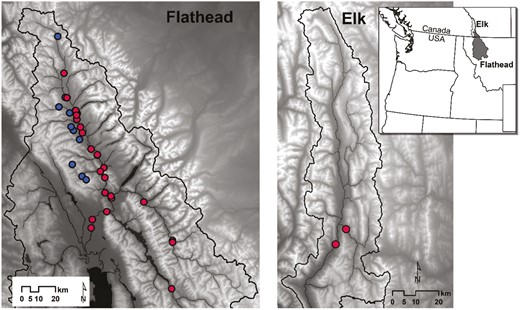
Map of all study sites sampled in the Flathead River, USA, and Elk River, Canada. Red points denote sites with only (or mainly) Sweltsa coloradensis. Blue points denote sites with only or mainly Sweltsa fidelis.
Species Distribution
Temperature is the strongest controller of species distributions in aquatic insects (Table 1). The abundance of dominant species is known to change along stream temperature gradients (Mani 1962;,Jacobsen et al. 1997; Hauer et al. 2001). Plecoptera in particular generally exhibit strong species segregation by temperature, with different species inhabiting colder versus warmer habitats (Stanford 1975; Hauer et al. 2001). Three species of Sweltsa (Family: Chloroperlidae) are known to occur at the elevations we sampled in the Flathead River system including S. coloradensis, S. fidelis, and S. revelstoka. Sweltsa coloradensis is the most widely distributed in lower elevation mainstem habitats. S. revelstoka is known to occur at the highest to mid-elevations in colder tributary habitats in Alberta and some males are brachypterous (reduced wings; Donald 1985). Within tributaries, S. fidelis occurs at mid-elevations, between S. coloradensis and S. revelstoka, and can have habitat overlap with S. revelstoka (Donald 1985). Sweltsa fidelis is also found in low-elevation cold water springs that can occur near mainstem habitats. Despite some habitat overlap, no previously known hybridization occurs between any of the Sweltsa species (Surdick 1995; Delk et al. 1998). Because nymphs of all Sweltsa species cannot be distinguished using morphology, we identified species (for nymphs) using genetic markers.
Environmental variables used in GEA tests for loci in Sweltsa with high genetic differentiation (FST)
| Environmental variable (description) | Biological mechanism(s) | References |
|---|---|---|
| Climate-related variables | ||
| Mean modeled June and July stream temperature (mean monthly stream temperature predictions for baseline period 1986–2005; Jones et al. 2014; 100 m pixels) | Stream temperature controls species distributions (based on life history strategies and physiological tolerance), egg development and hatching success, growth rates, emergence timing, fecundity, etc. | Nebeker 1971; Zwick 1980, 1981; Brittain 1990; Hauer et al. 2001; Fochetti and Tierno de Figueroa 2008; Merritt et al. 2008, Data Source: Jones et al. 2014 |
| Daily minimum air temperature (mean number of days until minimum air temperature reached 3.5 ° Ca for 2012–2017; Mean degree days from Jan 1st—June 7th for 2012–2017, 1 km pixels) | Air temperature influences stream temperature, snowpack and melt conditions, and emergence conditions. | Nebeker 1971; Hall et al. 2012, Data Source: Daymet (Thornton et al. 1997, 2012) |
| Total spring (Mar–May) precipitation (mm); Total summer (June–August) precipitation (mm, 1 km pixels) | Flow dynamics (flooding, flashiness, base flow) influence species distributions. | Statzner and Higler 1986 Data Source: Daymet (Thornton et al. 1997, 2012) |
| Snow cover (first snow free 8-day period, 500 m pixels) | Snow cover influences stream water temperature and the timing of snowmelt influences stream discharge. | Hall et al. 2012 Data Source: Hall et al. 2006 |
| Net primary productivity (NPP) (g C/year for 1 km pixels) | Increased production could increase organic debris inputs to streams (important energy sources). Macroinvertebrate communities change along a longitudinal downstream continuum (RCC). Woody debris shapes stream habitats, increasing habitat diversity and retaining allochthonous food resources. | Cummins 1974; Vannote et al. 1980; Bilby 1981; O’Connor 1991 Data Source: https://www.ntsg.umt.edu/files/modis/MOD17UsersGuide2015_v3.pdf |
| Habitat variables | ||
| Elevation (m) | Stream temperature changes with elevation. Stonefly species distributions and timing of emergence changes with elevation. | Mani 1962; Nebeker 1971; Kownacka and Kownacki 1972; Allan 1975; Vannote et al. 1980; Ward 1986; Jacobsen et al. 1997 Data Source: NED 10 m DEM (http://seamless.usgs.gov) |
| Aspectb | Aspect influences solar insolation which influences stream temperature, length of snow cover, growing conditions in riparian corridors, etc. | Nebeker 1971 Data Source: NED 10 m DEM (http://seamless.usgs.gov) |
| Slope (%) (from 30 m pixel) | Percent slope influences stream hydrology including discharge, substrate, habitat types, etc. | Statzner and Higler 1986 Data Source: NED 10 m DEM (http://seamless.usgs.gov) |
| Landcover (for 30 m pixel) | Landcover type influences runoff patterns, and flow affects stream plant and animal communities. Land use type (e.g., forestry vs. agriculture) influences sediment supply to streams, altering streambed habitat and influencing macroinvertebrate populations. | Lenat 1984; Menzel et al. 1984; Swanson et al. 1987; Bain et al. 1988; Statzner et al. 1988, Data Source: Yang et al. 2018 |
| Fire, year burned or no burn | Wildfire has short and long-term impacts on stream macroinvertebrate assemblages including altering species composition. | Minshall et al. 1989, 2001; Malison and Baxter 2010 Data Source: https://www.sciencebase.gov/catalog/item/5c991918e4b0b8a7f6288e05 |
References document how different environmental variables influence life history traits, abundance, and distribution of aquatic macroinvertebrates and stoneflies (Plecoptera) in particular. We reviewed the literature on potential biological mechanisms that may link environmental variables to variation in population-specific FST for neutral loci.
Emergence of Sweltsa was not documented at any sites until minimum air temperature reached 3.5 °C.
Aspect was transformed to measure “northness” using the cosine function so that a value of 1 corresponds to a north-facing stream, and −1 is a south-facing stream.
Study Design
To cover the maximum range of environmental variation that may drive selection in Sweltsa, we chose 50 study sites along an elevational gradient, from the mainstem Flathead (most downstream), up the Middle Fork and North Fork, and also on first-, second-, and third-order tributaries of the North Fork. We sampled each tributary in 2 locations (downstream and upstream) to maximize sampling over elevational gradients. This design allowed us to investigate potential differences in genetic structure of the 2 Sweltsa spp. populations at different spatial scales: within the watershed, between river forks, and between tributaries, as well as maximize environmental variation that may help detect selection signatures associated with different tributaries. Sample sites outside the Flathead, in the Elk River watershed, facilitated between watershed comparisons.
Sampling
We collected population samples of nymphs and adult Sweltsa spp. at all sites using a combination of kick net, rock pick, pitfall trap, and sweep net sampling methods between May–October 2017 (Supplementary Table S1). Nymphs were collected from stream sediments using a Stanford-Hauer kick net. Rocks were first scrubbed by hand and then the substrate was kicked to allow nymphs to float into the net. For rock-picking we flipped over rocks on the river bank and checked under them for late-instar and newly emerged adult Sweltsa spp.
We installed pitfall traps on river banks (on outside bends) to collect emerging adult Sweltsa spp. Coffee cans were buried so the top was flush with the ground and rocks were placed over them to block input of precipitation. We used ethylene glycol as a preservative in the traps. Each week all stoneflies were scooped out of all pitfall traps and placed in 95% ethanol. Adult Sweltsa were also collected by beating streamside vegetation with sweep nets. Adults emerged in the Flathead watershed from June—July of 2017. Periods of emergence lasted ~3 weeks at each individual site.
We collected all samples streamside, placed them in 95% ethanol, and returned to the laboratory for species or genus level identification under a dissecting microscope (Stewart and Stark 2002). Adult Sweltsa were identified to species and nymphs could only be morphologically identified to genus (Baumann et al. 1977). In total, we sampled 66 sites and collected Sweltsa spp. from 50 of those sites, but 12 of the 50 sites did not have sufficient sample sizes to be included in final data sets primarily due to admixture and poor sequencing quality (Supplementary Table S1).
Lab Methods
Total genomic DNA was extracted from stoneflies (after manually shredding the thoracic segment with sterile tweezers) using the high-throughput SPRI bead-based extraction protocol described in Ali et al. (2016), with Serapure beads (described in Rohland and Reich 2012) substituted for Ampure XP beads. DNA concentration was calculated using picogreen assays and DNA quality was assessed with a Nanodrop spectrophotometer. Libraries were sent to Novogene for sequencing. We produced sequencing data for 903 individuals (101 adults and 802 nymphs) from 50 sampling sites using RADseq to characterize the geographic and environmental patterns of neutral and potentially adaptive variation across populations. We sequenced 11 additional individuals from 3 locations (from sites nearby in Glacier National Park) that were morphologically identified for S. fidelis and S. revelstoka and used in comparison to our species diagnostic SNP marker sets (below). “BestRAD” libraries were prepared from genomic DNA, digested with the 8 bp cutter restriction enzyme SbfI and uniquely labeled using P7 index primers and in-line barcodes. We used an improved RAD protocol where biotinylated RAD adaptors bind to streptavidin-coated magnetic beads to improve recovery efficiency (Ali et al. 2016). The RAD libraries were then used as input into the NEBNext Ultra library kit from New England Biolabs. A single library was sequenced using 150 bp paired-end reads across 2 lanes on an Illumina HiSeq X machine.
Genome Assembly and Polishing
We used a Sweltsa nymph (sex unknown), captured live on the furthest downstream, lowest elevation, mainstem floodplain. Despite using a nymph, we were confident in the species distribution as S. coloradensis is known to inhabit low elevation mainstem habitats (Newell et al. 2008) and species identification was also later confirmed with genetic data. The nymph was gut evacuated for 48 h prior to being flash frozen and was sequenced with single-molecule real-time (SMRT) sequencing, developed by PacBio (Pacific BioSciences, California; https://www.pacb.com/) to create a long-read genome assembly. High weight molecular extraction and sequencing was performed at the Oregon State University’s Center for Genome Research and Biocomputing Core Facility using the continuous long reads (CLR) method. Pacbio sequencing produced 8 820 239 reads (87.9 Gb of total data) on a PacBio Sequel I machine (8 SMRT cells). We assembled the S. coloradensis genome using wtdbg2 (https://github.com/ruanjue/wtdbg2) with default settings and the Pacbio option for sequencing technology (option -x sq; Ruan and Li 2020).
From a second individual, a Sweltsa coloradensis adult male, we produced 324 660 085 total read pairs of Illumnia 150 bp paired-end whole genome shotgun sequencing, at 61× average coverage depth that was used for 2 rounds of assembly polishing (i.e., removal of sequencing errors). PCR duplicates in the Illumina data were filtered using clone_filter from the STACKs pipeline software tool to remove reads that had multiple identical first and second reads (Catchen et al. 2011, 2013). Illumina reads were then aligned to the consensus genome reference using BWA-MEM (Li 2013) and used to polish the assembly using wtdbg2. Genome completeness was assessed using BUSCO v3 and the 1658 “insecta_ob9” set of reference genes (Simão et al. 2015; Waterhouse et al. 2018) and assembly statistics were generated in Quast (Gurevich et al. 2013).
Overview of RAD-Seq Data Analysis
Initially we determined species clustering using 903 individuals from each of 50 sampling locations using the program STRUCTURE’s Q-values (Pritchard et al. 2000) to identify individuals belonging to 1 of 3 clusters corresponding with S. coloradensis, S. fidelis, and a third unidentified species, along with potential hybrid individuals. This initial SNP discovery was strictly used for species clustering and was done using de novo RAD-tag stack-building and genotyping in the program Stacks v2.1 (Rochette et al. 2019). We identified S. coloradensis using morphologically identified adults (66 total from 9 locations), and from repeated observational data and knowledge, as S. coloradensis is the only Sweltsa species that inhabits low-elevation, mainstem streams. To identify additional species in higher elevation tributaries, we sequenced adults morphologically identified as S. fidelis (N = 5) and S. revelstoka (N = 6).
After identifying locations with no admixture (i.e., Q ~ 1) from initial species clustering analysis, we used a subset of those individuals to discover species diagnostic marker sets to further assess admixture proportions for all individuals. Markers used for this discovery were taken from a set that was reference aligned to the S. coloradensis genome and genotyped using GATK. Non-admixed individuals (admixture < 95%) were then removed before determining polymorphic loci, and subsequent population and landscape genomics analyses, that were done independently for each species and using loci also genotyped using GATK. Mapping to the S. coloradensis reference genome for all individuals allowed for possible downstream comparison between diagnostic and polymorphic loci locations, and allowed comparisons (and potential annotation of specific genes) between species by using the same mapping reference.
RAD-seq Filtering and Trimming Prior to Genotyping
Prior to any genotyping, we assessed overall read quality using Fastqc (Andrews 2010) and trimmed all reads to 130 bp based on 90% of the bases having a Phred score >20. We used process_radtags (using the—bestrad option) from STACKs to sort reads by barcode, to rescue barcodes and RAD tags (-r option), and to remove any reads with an uncalled base (-c option), and discard reads with low quality scores (-q option). Other options used in process_radtags were the default where the barcode is inline with the sequence, only on the first read, and 1 mismatch is allowed when rescuing barcodes. PCR duplicates were removed using the clone_filter tool from the STACKs software package, version 2.1 on default settings and without a random oligo sequence (Catchen et al. 2013). Reads were then trimmed and filtered based on quality and length using Trimmomatic (Bolger et al. 2014). Adaptors were removed from reads, and a 4-base sliding window was used to trim the ends off reads when the average quality per base dropped below 15, with the minimum allowable read length being 60.
Species Clustering (De Novo in Stacks)
We conducted de novo stack assembly by following the protocol suggested by Rochette and Catchen (2017) for choosing the -m = 3, -M = 4 and -n = 4 parameters (used in ustacks and cstacks) for determining the minimum stack depth, the distance allowed between stacks and the distance allowed between catalog loci. Loci were then genotyped in gstacks. We used the populations module to filter loci using a minimum read depth of 8, minor allele frequency > 0.05, Ho < 0.6, and we required that loci were present in 50% of individuals in all sampling locations, and removed any individuals with >50% missingness. Loci discovery resulted in a set of 1537 SNPs for 725 individuals that were then used only to assess potential population structure (and species grouping for species-diagnostic discovery). We then ran the Structure program (Pritchard et al. 2000) with K = 1–10 and a burn-in period of 10 000 and 50 000 MCMC repetitions after burn-in. Finally, as an additional test, we plotted K = 3 with Q-values from the program Admixture and the associated cross-validation plot (Supplementary Figure S1).
RAD-Seq Alignment, Genotyping in GATK and Post Filtering
Post initial RAD-seq filtering, reads were aligned to our reference genome for S. coloradensis using BWA-MEM (Li 2013) with the default settings. Bam files were genotyped using HaplotypeCaller and the GATK incremental joint genotyping workflow (v3.7; Van der Auwera et al. 2013). All SNPs were filtered following GATK’s Hard Filtering Guidelines for non-model organisms using GATK’s VariantFiltration tool (Depristo et al. 2011; Van der Auwera et al. 2013). SNPs were filtered for quality by depth (QD < 2), root mean square of mapping quality (MQ < 40), mapping quality rank sum (MQRankSum < −12.5), read position rank sum test (ReadPosRankSum < −8.0), strand odds ratio (SOR > 3.0), genotype quality (GQ < 30), allelic balance (0.25 < AB > 0.75), and minimum depth (7 for homozygous SNPs and 10 for heterozygotes). Additionally, loci were filtered on minor allele frequency (MAF ≥ 0.05), and observed heterozygosity (HO < 0.6).
Species Diagnostic Marker Discovery
We first identified species-diagnostic loci for S. coloradensis and S. fidelis (with alleles fixed or nearly-fixed within species); later we identify polymorphic loci within species (see next section). STRUCTURE’s Q-values (Pritchard et al. 2000) from the species clustering were used to determine initial admixture proportion in choosing putatively non-admixed individuals to use for ascertainment of species-specific loci. We selected up to 3 individuals from each site with q = 1 and the smallest number of missing genotypes (max 50%). Diagnostic SNPs for the 3 “species” (clusters) were identified as shared bi-allelic loci with strict segregation of alleles, with pair-wise FST > 0.9 between S. coloradensis and the other 2 species, and less than 10% missing genotypes. We then estimated admixture for all individuals using the 3 newly identified sets of diagnostic loci. Using the set of all non-admixed individuals we calculated pairwise FST values between the putative species groups using Genepop v4.1.4 (Rousset 2008).
Polymorphic Loci Discovery in Each Species (with a Reference Genome and GATK)
After removing admixed individuals (>5% admixture), 373 S. coloradensis and 153 S. fidelis across 40 sampling locations remained. With that subset of individuals, we further developed 2 sets of polymorphic loci (one for S. coloradensis and S. fidelis each). Our 2 ascertainment panels included up to 2 non-admixed individuals from each sampling location (n = 27 S. coloradensis locations, n = 13 S. fidelis). For each species, we refined our data set of all filtered variable SNPs identified previously by excluding all species diagnostic loci (monomorphic within species), loci with an MAF <0.05, or with data missingness >20% and loci with >40% missing data within a sampling location, and by excluding individuals with data missingness >50%. Lastly, we used HDplot to remove potential paralogous loci (McKinney et al. 2017). SNPs, where the read ratio deviation (D > 20) or the proportion of heterozygotes (H > 0.6) exceeded these thresholds, were assumed to be duplicated and removed. All sampling locations with less than 5 individuals were removed before analysis for both species.
We tested for Hardy–Weinberg proportions (HWP) and computed FIS in R (R Core Team 2020) using the “adegenet,” “pegas,” and “hierfstat” packages (Jombart 2008; Paradis 2010; Jombart and Ahmed 2011; Goudet and Jombart 2021). We tested for HWP using the Exact test with 1000 Monte Carlo replicates (Guo and Thompson 1992) and the Bonferroni false discovery rate correction in the “stats” R package. We assessed HWP and FIS using only populations with >10 individuals and removed loci deviating from HWP after Bonferroni correction or if the absolute value of FIS ≥0.9 in more than 3 populations. We plotted the final scatterplot distribution of FIS values for S. coloradensis and S. fidelis (Supplementary Figures S5 and S6).
For each species, we also produced a second, less stringently filtered data set to use for testing for selection and landscape genomics analyses. The purpose of the less stringent data set was to identify more candidate adaptive outlier loci (and avoid inadvertently filtering out loci under selection). The only difference between stringency was how the data set was filtered for LD. For the more stringent data set, we kept only one random SNP per RAD-tag. For the second data set, we filtered out loci with high linkage disequilibrium (LD), similar to (Yadav et al. 2021), where if R2 >0.7 in 5 (for S. coloradensis) or 2 (for S. fidelis) or more sampling locations (with ≥15 individuals) then we then removed one of the loci in the pair. LD R2 values were calculated using Plink v1.90 (Chang et al. 2015).
Influence of River Network Structure on Gene Flow and Genetic Diversity
River networks are highly hierarchical in structure and the null hypothesis is that river distance is the main driver of genetic structure for aquatic species that primarily disperse via the river network (Morrissey and De Kerckhove 2009; Altermatt 2013; Fronhofer and Altermatt 2017). We tested for genetic isolation by distance using both river distance and Euclidean distance with Mantel tests (Mantel 1967) in the “vegan” R package (Oksanen et al. 2020). We used the National Hydrography Data set (NHD; http://nhd.usgs.gov) to calculate the river distances between the sample sites. Pairwise FST values were correlated with matrices of population pairwise river distances and population pairwise Euclidean distances. Population pairwise fixation index (FST) values were calculated using the Weir and Cockerham (1984) method in the R-package “hierfstat.” Median global FST for each species was calculated for all loci using Nei (1987) method in the R-package “heirfstat.” For these analyses and for the remainder of this section, we used only the more stringent data set.
To further test the influence of river network structure on gene flow we also performed principal component analysis (PCA) to identify clusters of individuals, assuming that individuals would cluster mainly by sampling location if gene flow was limited. PCAs used individual allele frequencies to identify potential population structure within each species and among sampling sites. PCAs were performed using the “adegenet” package for scaling (function scaleGen) and the “ade4” package (Dray and Dufour 2007) for the PCA (function dudi.pca).
We tested for population genetic clustering using the Admixture program (Alexander et al. 2009). We used the default settings and the 5-fold cross validation error to determine the most likely value for K. For our range of possible K values, we used from 1 to the number of sampling locations for each species. We also compared our results using discriminant analysis of principal components (DAPC; Jombart et al. 2010) as implemented in the “adegenet” package (function find.clusters). The DAPC test uses the model with the maximum Bayesian information criterion (BIC) to choose the best supported number of clusters (K). DAPC differs from PCA in attempting to maximize between-group variation, but unlike PCA also attempts to minimize within-group variation (Jombart et al. 2010).
For population genetic analyses, we removed 6 sampling locations from the data set because there were not enough individuals (n < 5), identified as a single species at >95% of diagnostic markers, available for population and landscape genomic analyses. Site-based population genetic measures observed and expected heterozygosity, and allelic richness (HO, HE, Ar) were calculated with the R package “diveRsity” (Keenan et al. 2013; Table 3). We used a t-test to test for significant differences in HE between the 2 species.
Summary statistics for each sampling location within the mainstem Flathead River and the 3 major drainages of the Flathead River (Middle, North, and South Fork), as well as the Elk River
| Sweltsa coloradensis | Sweltsa fidelis | ||||||||||
|---|---|---|---|---|---|---|---|---|---|---|---|
| Population | n | H O | H E | F IS | Ar | Population | n | H O | H E | F IS | Ar |
| Main Flathead River | |||||||||||
| PR | 7 | 0.260 | 0.258 | −0.018 | 1.66 | ||||||
| KBMS | 13 | 0.271 | 0.264 | −0.018 | 1.68 | ||||||
| CBMS | 8 | 0.265 | 0.258 | −0.031 | 1.66 | ||||||
| BKMS | 18 | 0.280 | 0.273 | −0.018 | 1.69 | ||||||
| BLMS | 17 | 0.282 | 0.273 | −0.031 | 1.69 | ||||||
| Middle Fork Flathead River | |||||||||||
| MR | 7 | 0.268 | 0.256 | −0.05 | 1.65 | ||||||
| DT | 5 | 0.268 | 0.242 | −0.112 | 1.6 | ||||||
| BC | 17 | 0.273 | 0.271 | −0.002 | 1.7 | ||||||
| North Fork Flathead River | |||||||||||
| UT | 10 | 0.275 | 0.265 | −0.038 | 1.66 | SKTD | 18 | 0.217 | 0.208 | −0.029 | 1.60 |
| GNMS | 9 | 0.331 | 0.281 | −0.149 | 1.68 | SKTU | 9 | 0.215 | 0.2 | −0.064 | 1.56 |
| CC | 11 | 0.307 | 0.279 | −0.086 | 1.68 | KLTU | 17 | 0.216 | 0.207 | −0.023 | 1.59 |
| BGTD | 15 | 0.295 | 0.277 | −0.057 | 1.66 | HATU | 10 | 0.221 | 0.2 | −0.077 | 1.57 |
| COTD | 10 | 0.27 | 0.264 | −0.024 | 1.69 | RMTU | 14 | 0.233 | 0.211 | −0.069 | 1.60 |
| COMS | 13 | 0.281 | 0.269 | −0.035 | 1.66 | MCTU | 15 | 0.216 | 0.205 | −0.03 | 1.55 |
| HAMS | 16 | 0.271 | 0.271 | 0.002 | 1.72 | TPTD | 14 | 0.222 | 0.21 | −0.041 | 1.60 |
| RMMS | 18 | 0.278 | 0.272 | −0.013 | 1.7 | TPTU | 12 | 0.222 | 0.203 | −0.064 | 1.56 |
| MCMS | 17 | 0.282 | 0.273 | −0.027 | 1.69 | KTTD | 11 | 0.22 | 0.199 | −0.082 | 1.56 |
| TPMS | 12 | 0.282 | 0.266 | −0.053 | 1.65 | KTTU | 15 | 0.227 | 0.216 | −0.033 | 1.61 |
| LW | 14 | 0.271 | 0.267 | −0.012 | 1.67 | CLTU | 12 | 0.231 | 0.214 | −0.063 | 1.58 |
| WU-1 | 16 | 0.283 | 0.273 | −0.028 | 1.68 | PO | 6 | 0.215 | 0.19 | −0.116 | 1.52 |
| WU-2 | 17 | 0.269 | 0.267 | 0.000 | 1.68 | ||||||
| MD | 10 | 0.271 | 0.263 | −0.036 | 1.67 | ||||||
| KTMS | 10 | 0.276 | 0.261 | −0.054 | 1.66 | ||||||
| CLMS | 15 | 0.279 | 0.268 | −0.039 | 1.65 | ||||||
| BT | 14 | 0.278 | 0.271 | −0.021 | 1.69 | ||||||
| South Fork Flathead River | |||||||||||
| RD | 18 | 0.271 | 0.271 | 0.005 | 1.69 | ||||||
| Elk River | |||||||||||
| MC | 19 | 0.256 | 0.268 | 0.044 | 1.71 | ||||||
| SP | 16 | 0.256 | 0.265 | 0.032 | 1.7 | ||||||
Within each basin, sampling locations are ordered approximately from the most downstream to the most upstream point (Figure 2). The presence of TD or TU in a site code denotes tributary habitat, all other sites are located in main channel habitat. n = the number of individuals included in analyses, and HE and HO are expected and observed heterozygosity, respectively. FIS measures deviation from HW proportions.
Outlier Detection, Landscape Genomics, and Environmental Data
We first conducted outlier detection (using only the less stringently filtered data set and without environmental data) to estimate the probability that each locus is influenced by natural selection. This was done using a Bayesian framework in BAYESCAN v2.1 to estimate probabilities based on allele frequencies between populations as measured by a subpopulation-specific FST (Foll and Gaggiotti 2008). We used default settings for BAYESCAN v2.1 which include 20 pilot runs (5000 iterations in length) followed by a burn-in of 50 000 iterations and a final run of 100 000 iterations. We used a conservative false discovery rate (FDR) of 0.05 to identify putative outlier loci. BAYESCAN plots were produced using the provided plot_bayescan R script.
In addition to an FST outlier test, we used a genotype–environment associations (GEA) method to incorporate environmental variation into tests for loci influenced by natural selection (Rellstab et al. 2015; Balkenhol et al. 2017; Forester et al. 2018a). Following Forester et al. (2018b), we choose a multivariate ordination technique, redundancy analysis (RDA), which can be used to analyze many loci and environmental predictors simultaneously (Legendre and Legendre 2012; Borcard et al. 2018). This can account for many loci of small effects (polygenic) resulting from weak, multilocus selection signatures. Forester et al. (2018a, 2018b) showed that RDA was sufficient and “superior” to other GEAs with low false-positive rates and the highest rates for true positives. Also, under weak population structure as we have in this study (see results for more information), Forester et al. (2018a, 2018b) also demonstrated that an unconstrained RDA performed better than pRDA.
The first step in RDA is to perform a multivariate linear regression using genetic and environmental data which produces a matrix of fitted values of the response variables. The second step is a constrained version of PCA where the canonical axes are linear combinations of the explanatory variables (Legendre and Legendre 2012). RDA can be used to analyze genomic data on an individual (using genotypes) or population level (using allele frequencies). We did not have individual geospatial data as all individuals were collected within a single sampling location, hence, we used a population level RDA. Sampling location level allele frequencies were calculated for each sampling site in the “hierfstat” package, and the RDA was performed and plotted using the “vegan” package. Overall model significance, and each constrained axis, were tested using F-statistics and an ANOVA-like permutation test using 9999 permutations of the response variable for RDA to assess the significance of constraints (anova.cca in the “vegan” package). The P value threshold of 0.05 was used.
We used the RDA constrained axis SNP loadings (the contribution of each SNP to the vector associated with a given constrained axis where strong loadings are SNPs more highly correlated with a specific environmental variable) to identify candidate adaptive loci using the method as described in Forester et al. (2018a, 2018b) by considering SNPs loading ±2.5 standard deviations (2-tailed P value = 0.012) from the mean loading of the first axis, and any other axes that were significant. The most strongly correlated environmental covariate was then chosen for each candidate SNP to visually group the outlier loci when plotting.
We selected environmental data for the GEA analysis that may influence the local conditions important to the physiology and ecology of stoneflies (Table 1). Stonefly species distributions, life history, and physiology are most strongly influenced by the temperature, flow, and oxygen of their habitats (Allan and Castillo 2007). Water temperature exerts one of the strongest controls on stonefly emergence and distribution outside of the appropriate photoperiod stimulus (Nebeker 1971; Brittain 1990). Emergence occurs for each species at specific temperature cues, beginning at lower elevations from warmer water and starting later at increasing elevations (Nebeker 1971). Air temperature also influences emergence timing and we used 2 different air temperature metrics.
First, we determined the minimum air temperature at which emergence of Sweltsa occurred at a subset of our sites and then calculated the mean days to that minimum air temperature (3.5 °C; Supplementary Table S2). For the second air temperature metric we calculated the degree days accumulated for each site by the beginning of the Sweltsa emergence period in the Flathead drainage (starting 7th June). We also included other climate related variables that could influence Sweltsa populations including precipitation, snow cover and net primary productivity (Table 1). Landscape level features (e.g., elevation, aspect, slope, landcover, etc.) also strongly influence physical characteristics of different sites. For example, aspect influences solar insolation and snow and ice cover which influences water temperature and the timing of emergence. As many environmental predictors can be highly collinear (R > |0.7|; Dormann et al. 2013), we pruned predictors using a pairwise correlation matrix (using the pairs.panels function from the “psych” R package) and retained the variable most relevant or ecologically interpretable (Revelle 2021). Correlation testing was performed for each species independently and a cut off of R = 0.7 was used.
Gene Annotation with BLAST
We searched for candidate genes near putatively adaptive SNP loci identified by the GEA and FST outlier approaches using the NCBI BLAST web platform (Johnson et al. 2008). We first used the reference genome to pull the 500 bp of nucleotide sequence flanking each of the candidate adaptive SNPs, and used only one sequence for each unique RAD tag. Nucleotide sequences were then translated to proteins with the BLASTX web tool in each of the 6 possible reading frames (to account for an unknown starting point for protein translation). We did a non-redundant protein database search (default on the BLASTX webtool) with the translated nucleotide sequences and kept database hits that had an E-value < 1 × 10⁻⁴, were identified in an organism in class Insecta, and maintained the same reading frame across the top 10 significant (E-value < 1 × 10⁻⁴), organism hits. We report the number of significant hits and the potential known function for relevant hits.
Results
Sweltsa Reference Genome
We produced the most complete reference genome available for a stonefly, S. coloradensis, using an average sequencing depth of coverage =35× (with PacBio) and an average kmer depth =39 (Table 2). The final genome reference size was 1.48 Gb with 21 523 total contigs (L50 = 1276) and the largest contig size = 6.03 Mb and N50 = 0.251 Mbp. BUSCO scores suggested a nearly complete coding gene assembly (95.2% complete [single- and double-copy genes], 2.2% fragmented genes, and 2.6% missing BUSCO genes). All associated data for the resources detailed in this study, including both raw reads and assembly, are available as part of GenBank BioProject PRJNA843028.
Genome assembly statistics
| Metric | Sweltsa coloradensis |
|---|---|
| Coverage | 35× |
| Ave. Kmer depth | 39 |
| Assembly size | 1.48 Gbp |
| Total contigs | 21 523 |
| Largest contig | 6.03 Mbp |
| N50 (contig) | 0.251 Mbp |
| L50 (contig) | 1276 |
| N75 (contig) | 0.07 Mbp |
| L75 (contig) | 4263 |
| Complete BUSCOs | 1580 (95.2%) |
| Single copy | 1488 |
| Duplicated | 92 |
| Fragmented BUSCOs | 37 (2.2%) |
| Missing BUSCOs | 41 (2.6%) |
N50 is the sequence length of the shortest contig of the set of contigs that represent 50% of the total genome length. L50 is the length of the contig in the set of contigs whose length sum makes up half of genome size.
RAD-Seq SNP Discovery, Genotyping, and Filtering
We identified 3996 polymorphic SNPs for S. coloradensis among 373 individuals (including only individuals with ≤5% admixture as identified from species-diagnostic SNPs) across 28 sampling locations. We retained a total of 1930 polymorphic SNPs and 372 individuals in the more stringent data set (Supplementary Table S3). No loci were removed because of deviations from HWP or FIS-based tests. For the less stringently filtered data set (for landscape genomics and selection detection), the number of individuals and locations were the same, but we retained more SNPS (e.g., 3454 SNPs; Supplementary Table S4).
For S. fidelis, we identified a total of 1713 polymorphic SNPs in 153 individuals across 12 sampling locations after filtering based on 5% admixture. Of the SNPs removed, 36 SNPs were taken out of both stringency data sets based on deviation from HWP and FIS-based outlier tests (Supplementary Tables S3 and S4). For both data sets, we retained all individuals and sampling locations, resulting in 520 polymorphic SNPs for the more stringent filtering and 1070 for the less-stringently filtered data set (Supplementary Tables S3 and S4).
Species Distribution and Hybridization
Using the initial RAD data set with all individuals, we detected 3 distinct clusters (putative species) using STRUCTURE and high pairwise FST values ranging from 0.883 to 0.886 between the 3 clusters (Supplementary Table S3, Supplementary Figure S2). Among individuals we detected substantial amounts of low-level hybridization between S. coloradensis and S. fidelis (predominantly S. fidelis individuals with 1–4% S. coloradensis), as well as potential hybridization between S. fidelis and a third unknown species (UNKNOWN1—morphological identification was not possible because we had no adult samples and nymphs can only be identified to genus). Forty-four individuals were identified across 11 sites with predominately UNKNOWN1 alleles (proportion of UNKNOWN1 alleles > 0.95). Across 53 sites, 26 had predominately S. coloradensis individuals (proportion of S. coloradensis alleles (pSC) ≥ 0.95), while 6 sites had predominately S. fidelis individuals and 1 site had a majority of UNKNOWN1 individuals from an apparent 3rd species.
In our analysis, the 66 adults morphologically identified as S. coloradensis from 9 mainstem sampling locations were identified to also have ≥99% of species diagnostic markers associated with S. coloradensis. The remaining samples used in this study were nymphs, which were not possible to morphologically identify to species, and hence, it was confirmed after sequencing that S. fidelis was present in the tributaries and surprisingly that another unknown Sweltsa species (UNKNOWN1) was also present in the tributaries. Also, as part of our analysis, we included a small set of morphologically identified S. fidelis adults and S. revelstoka adults because they are known to occur in tributary habitats. We found that for S. fidelis, 4 of the 5 individual adults had >99% of the tributary related species diagnostic markers. This led us to conclude that S. fidelis is the secondary species sampled in tributaries, but there is potential hybridization with UNKNOWN1 as we had one S. fidelis identified individual that appeared to be an F1 hybrid having a roughly 50%/55% split of S. fidelis and UNKNOWN1 (not S. revelstoka) in terms of species diagnostic markers. Attempts to identify to UNKNOWN1 were inconclusive because S. revelstoka identified adults did not match up completely with UNKNOWN1 and instead, were roughly distributed and had species diagnostic markers representing both S. fidelis (from 18% to 42%) and UNKNOWN1 (from 6% to 53%).
Genetic Diversity and Gene Flow in Mainstem and Tributary Habitats
Differences in genetic diversity (HE) between the 2 species (S. coloradensis and S. fidelis) were significant (0.267 ± 0.008 vs. 0.205 ± 0.007; t = 2.030, P < 0.001). Overall, HE was 24% lower in S. fidelis compared to S. coloradensis (ranging 0.261–0.281 in all sampling locations for S. coloradensis compared to 0.19–0.216 for S. fidelis). For both species, many sampling locations had an excess of heterozygotes (HO > HE) and mostly negative FIS values. One notable exception was the Elk River for which both sampling locations had slightly positive FIS values. The Elk River is geographically adjacent to the North Fork Flathead drainage (Figure 1).
Genetic differentiation between pairwise sampling locations was low for S. coloradensis across the sampling range (population pairwise FST = 0.000–0.014; global median FST = 0.000; Supplementary Table S5), including the Elk River. For S. coloradensis, there was no discernable difference in genetic differentiation between watersheds (the Flathead River vs. the Elk River), within the Flathead watershed (i.e., multiple forks including the North, Middle, and South Fork of the Flathead), or within the forks of the Flathead River (Supplementary Table S5). For S. coloradensis, Mantel tests showed that genetic differentiation was positively correlated for both river distance (R = 0.26, P = 0.014) and Euclidean distance (R = 0.449, P = 0.001).
S. fidelis also had low population pairwise genetic differentiation (FST = 0.000–0.028) and a low global FST median (FST = 0.000) across sampling locations (Supplementary Table S6). Two of the tributary locations, CLTU and TPTD, had higher genetic differentiation than the rest of the S. fidelis sites (Supplementary Table S6). Mantel tests were not significant for river distance (R = 0.020, P = 0.371) or Euclidean distance (R = 0.0556, P = 0.299).
PCAs showed little clustering by sample location and were low in explanatory power (Figure 3). For S. coloradensis the first PCA axis only explained 4.27% of variation, and for S. fidelis the first PCA axis explained only 4.68% of the variance. Admixture results were similar in support of a K = 1 value for both species, with K = 1 having the lowest cross validation error in both species (Supplementary Figure S4). Finally, the minimum value of BIC in the DAPC tests also occurred at K = 1 for both species, therefore, we do not cover it further here.
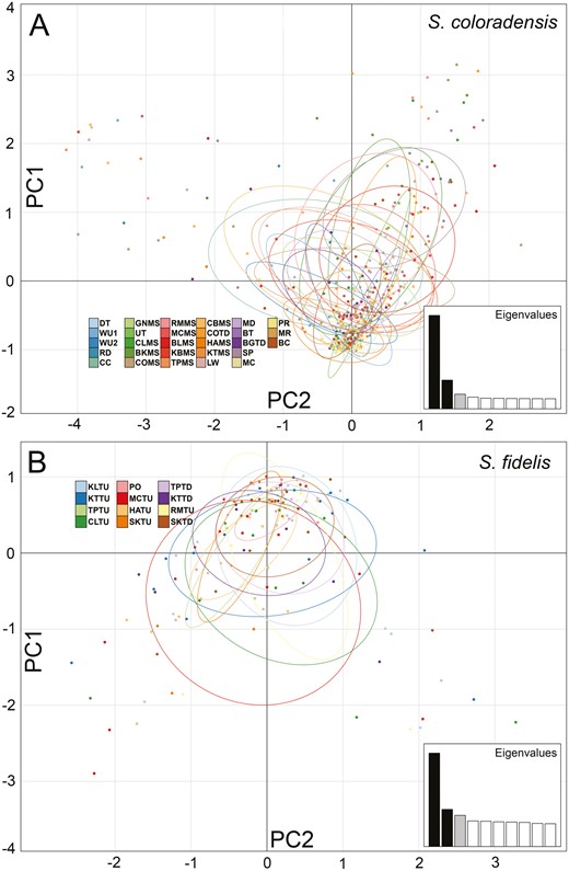
Individual-based PCA plots of population structure with environmental variables for (A) Sweltsa coloradensis and (B) Sweltsa fidelis. Largest 3 raw eigenvalues (and % variance explained) were 164.57 (4.27), 50.59 (1.31), and 25.81 (0.67) for S. coloradensis and were 48.36 (4.68), 19.26 (1.86), and 16.15 (1.56) for S. fidelis.
Outlier Detection, Landscape Genomics, and Candidate Adaptive Loci
Using the less stringently filtered data set, BAYESCAN identified 63 outlier loci on 49 unique RAD tags for S. coloradensis and 13 candidate outlier loci on 8 unique RAD tags for S. fidelis (Supplementary Figures S7 and S8). These outliers were mapped to the S. coloradensis reference genome, and were located on 40 contigs for S. coloradensis and 7 contigs for S. fidelis. Sweltsa coloradensis had 3 contigs each with 4 or more outlier loci, while S. fidelis had 1 contig with 5 outlier loci. S. coloradensis had 15 outliers that were above FST = 0.1 (maximum FST = 0.30) while S. fidelis only had a single outlier above FST = 0.1 (maximum FST = 0.13).
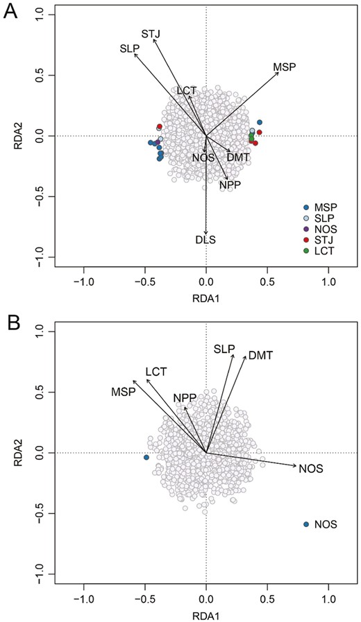
Our RDA model for S. coloradensis contained 8 environmental predictor variables including landcover type, aspect, slope, NPP, mean summer precipitation, days to last snow cover, mean June stream temperature and mean days to a minimum temperature for emergence (using the less stringent data set; Figure 4A). The model for S. coloradensis explained only 2.6% of model variance when adjusted for the number of predictors, but was significant (Pr(>F) = 0.048) based on the ANOVA, assuming a significance level of 0.05. Neither of the first 2 constrained axes were significant by themselves (Pr(>F) = 0.085 for the first axis and Pr(>F) = 0.248 for the second axis).

Population-level RDA plots showing the relationship between environmental covariates and sampling sites for (A) Sweltsa coloradensis and (B) Sweltsa fidelis. Environmental covariates include: NPP, net primary productivity; MSP, mean summer precipitation; LCT, land cover type; SLP, slope; DMT, mean days to minimum temperature; NOS, northness; STJ, mean June stream temperature; DLS, days to last snow cover. Arrows show the strength of the relationship between each environmental variable and the constrained axes.
The S. fidelis model included 6 environmental variables after pruning: landcover type, aspect, slope, NPP, mean summer precipitation, and days to a minimum temperature for emergence (Figure 4B). The model for S. fidelis explained 6.3% of total model variation when adjusted for the number of predictor variables. The model was not significant (Pr(>F) = 0.103) based on the ANOVA, and first 2 constrained axes were also not significant by themselves (Pr(>F) = 106 for the first axis and Pr(>F) = 0.564 for the second axis).
SNP loadings from the RDA models identified 19 outlier SNPs for S. coloradensis, associated most strongly with mean summer precipitation (MSP, 9 total), mean June stream temperature (STJ, 4 total), slope (SLP, 3 total), landcover type (LCT, 2 total) and aspect (NOS, 1 total) (Figure 5A). No outlier SNPs for S. coloradensis were on the same reference contig. For S. fidelis, there was one outlier SNP, associated with NOS, detected using the RDA model (Figure 5B).
SNP-based variation associated with environmental covariates from RDA analysis for (A) Sweltsa coloradensis and (B) Sweltsa fidelis. NPP, net primary productivity, MSP, mean summer precipitation; LCT, land cover type; SLP, slope; DMT, mean days to minimum temperature; NOS, northness; STJ, mean June stream temperature; DLS, days to last snow cover. Arrows show the strength of the relationship between each environmental variable and the constrained axes.
Gene Annotations with BLAST
For S. coloradensis, we found significant hits in non-redundant protein databases for 13 of our candidate adaptive SNPs identified in BAYESCAN and 1 of those identified using GEA. Of significant hits from BAYESCAN results, a majority were of unknown function, however of the genes of potentially known function in other species included genes important in sensory neurons (soluble guanylate cyclase gcy-37), cell apoptosis (caspase-2-like), and metabolism of insect hormones (cytochrome P450 4C1). The single identified gene for S. coloradensis has a potential function important in cell function (golgin subfamily A member 2 isoform X2).
For S. fidelis, there were 4 significant gene hits output by BLASTX identified for the BAYESCAN model results, and none for the GEA approach. Of the 4 significant gene hits for BAYESCAN, there was one gene with potential known function that included multiple molecular functions (adenylate cyclase type 6).
Discussion
This study suggests that the location of a Sweltsa species along the river network (mainstem vs. higher-elevation tributaries) influences the genetic diversity within Sweltsa species but not genetic subdivision and population connectivity. There were differences in genetic diversity (heterozygosity) in the 2 closely related stonefly species, but FST was near zero in both species. The PCA showed little genetic clustering of individuals and the near-zero FST values supported high connectivity among locations within the drainage for each species, despite differences in their distribution.
Climate change is predicted to influence population genetic connectivity of many terrestrial and aquatic species (Wasserman et al. 2013; Jaeger et al. 2014; Inoue and Berg 2017). It is also predicted that climate change will force many species to shift their ranges, but it is unclear whether many will be able to shift their geographic distributions fast enough (Loarie et al. 2009; Chen et al. 2011; Razgour 2015). Additionally, species differences in niche breadth can influence adaptive capacity (Yadav et al. 2021). Range shift capacity can be inferred from dispersal, gene flow, and genetic structure. In this study, we quantified structure and identified a set of environmental variables (landcover type, aspect, slope, NPP) and climate related variables (mean summer precipitation and days to a minimum temperature for emergence) that help explain patterns of genetic differentiation in both the mainstem and tributary species.
Genetic Diversity and Differentiation
The significant differences in HE between species (HE = 0.267 vs. 0.205) likely do not result mainly from differences in connectivity because mean FST values were near zero, rather differences in HE might be driven by other factors like differences in Ne between the 2 species. The more downstream species, S. coloradensis, had higher HE compared to the upstream S. fidelis, which aligns with other work documenting downstream increases in genetic diversity (Alp et al. 2012; Paz-Vinas et al. 2015). The average HO is also higher in S. coloradensis, but we use HE because it is a more appropriate measure of population diversity (gene diversity) than HO (Nei 1987).
Contrary to our prediction that S. fidelis are more isolated (i.e., lower landscape connectivity) in high elevation tributaries, our results suggest similar levels of genetic connectivity for both Sweltsa spp. Multiple clustering algorithms (PCA, DAPC, and Admixture) did not detect genetic structure or subdivision (i.e., no clear clustering of individuals) for mainstem S. coloradensis or tributary S. fidelis (K = 1 population cluster when considering all sampling locations for both species), suggesting that gene flow is high in both habitats. Interestingly, this was even the case for S. coloradensis between samples from adjacent watersheds that are isolated by mountains (the Flathead and Elk Rivers), with waters that only converge hundreds of miles downstream in the Columbia River Basin, offering further support of high connectivity. This is consistent with the global mean FST found to equal zero despite a significant result for the Mantel test indicating genetic differentiation between sampling locations did increase with distance for S. coloradensis (both Euclidean and river distance) but overall population pairwise FST values were very low (Supplementary Table S5 and S6). In light of the other clustering results agreement (PCA, DAPC, and Admixture) of K = 1 and a lack of population genetic structure, the Mantel test result is likely not very informative in this system and is mainly provided for completeness. Previous work on aquatic insects has found that genetic differentiation is not a function of geographic distance because flight is a major mechanism of movement at large spatial scales (i.e., between drainages; Sweeney et al. 1986; Jackson and Resh 1992; Schmidt et al. 1995; Hughes et al. 1998).
For most sites, we observed negative FIS values (Supplementary Figures S5 and S6). This might be explained by multiple factors. First, sampling mostly nymphs (before dispersal), can cause negative FIS because certain social structures, inbreeding avoidance, and long-distance dispersal can lead to an excess of heterozygotes (negative FIS), which is generally stronger in juveniles (before dispersal; Basset et al. 2001; Parreira and Chikhi 2015). This excess of heterozygotes can result from parents being relatively genetically distinct (e.g., allele frequency differences in parents). FIS values in locations where most individuals sampled were adults (PR, BC, UT, CC, LW) were close to zero (except CC had FIS = −0.38; Table 3).
Other factors that might contribute to the negative FIS values include polygamy and sex-biased dispersal (Basset et al. 2001; Parreira and Chikhi 2015). Negative FIS could also result from natural selection or technical issues in scoring the genotypes (Graffelman et al. 2017). However, natural selection (balancing selection) does not generally affect numerous loci and thus would unlikely shift the FIS distribution. We carefully filtered to remove loci with technical issues potentially causing excess of heterozygotes. For example, we filtered to remove duplicated genes to prevent paralogues (or 2 loci collapsed together as one) from contributing to an excess of heterozygotes. Small effective number of breeders can cause negative FIS but is unlikely here (Allendorf et al. 2013).
Candidate Loci Under Selection and Landscape Genomics
For this work, we produced a nearly complete reference genome (95.2% gene completeness in BUSCO) for a stonefly species (also see Hotaling et al. 2019). We used the reference genome to facilitate RAD genotyping, testing for selection, and to locate genome regions under selection. Shafer et al. (2017) conducted an extensive test of the bioinformatics pipeline to understand the bias associated with using a de novo versus mapping to references of increasing divergence. Here, we followed the recommendation of Shafer et al. (2017), to use a closely related reference genome, which should decrease bias in most summary statistics (over the de novo approach). The reference-based approach also has the major advantage of keeping mapping information comparable between species to identify genes and regions that are similar between species (and to identify paralogs). However, there is always some amount of decrease in mapping percentage when using a closely related species over using the species-specific reference genome, but the overall number of SNPs retained is higher than de novo assembly. This in part would explain the discrepancy in the number of SNPs discovered for each species along with other factors such as the number of sites sampled and the differences in genetic diversity. The lower number of putatively adaptive loci identified in S. fidelis would also be partially explained by these factors, but also because all locations for S. fidelis were in the same river drainage (vs. locations for S. coloradensis being in multiple drainages).
For both S. coloradensis and S. fidelis, the program BAYESCAN identified more than twice the number of outliers than the GEA approach. FST outlier methods often identify more false positives which could account for some of the additional significant loci (De Mita et al. 2013). One potential reason that the GEA detected fewer candidate adaptive (outlier) loci is that additional important factors were not considered by the environmental data such as behavior and demography-related influences. There was some evidence BAYESCAN identified genes important in sensory and metabolism function, however, a more detailed annotation and higher density of markers across the genome is needed to add strength to this hypothesis.
Environmental variation potentially influences adaptive genetic variation. In our study we had limited power to detect potential adaptive loci due to low density of genome-wide loci. Despite this, we discovered multiple landscape and climate-related variables that were correlated with adaptive genetic variation for S. coloradensis (and one variable for S. fidelis). Unsurprisingly, aspect (abbreviated NOS for northness in our model) was an important environmental variable in models for both species. Aspect influences stream temperature, one of the most important drivers of aquatic invertebrate species distributions (Table 1). For S. coloradensis, additional environmental variables were important. Slope directly influences stream hydrology and habitat availability (Table 1). Landcover type influences runoff, sediment and wood supply, all of which influence habitat and food resources (Table 1). Important climate-related variables included mean summer precipitation, and mean June summer temperature. Precipitation influences flow dynamics and habitat and temperature strongly influences species distributions and timing of emergence (Table 1).
For both species, RDAs using the final set of 1930 and 520 SNPs (from S. coloradensis and S. fidelis, respectively) showed that a small portion of variation in allele frequency (among loci) was explained by environmental variables (2.7% for S. coloradensis and 6.6% for S. fidelis). SNP loadings for S. coloradensis identified 10 putative candidate loci that were most strongly associated with mean summer precipitation, slope, and aspect. Given that 8 of the 10 putative loci under selection were associated with mean summer precipitation, it is possible that precipitation and flow dynamics are more influential in local adaptation than other environmental factors, however, this is with some caveats. None of the 10 outlier loci were located on the same contig (N50 = 0.251 Mbp). Given the large genome size for S. coloradensis (1.48 Gbp), and assuming a similar genome size for the closely related S. fidelis, it is possible that the relatively few outlier loci detected for S. coloradensis, and especially for S. fidelis, results from marker density being too low compared to rates of linkage disequilibrium (Lowry et al. 2017). Local adaptation is still potentially occurring for S. fidelis in tributary habitats even though it was not observed here.
Species Distributions and Introgression
We detected only limited hybridization between S. coloradensis and S. fidelis, as well as potential hybridization between S. fidelis and one other genetically distinct “species” (“UNKNOWN1”) that we could not morphologically identify (no adult samples, with our nymphs only identifiable to genus). S. coloradensis was most widely distributed, while S. fidelis was predominately at higher elevation headwater sites. Limited hybridization (e.g., 0.88 < pSF < 0.98) between S. fidelis and S. coloradensis was most common, with little evidence for recent admixture events observed. This discovery is interesting because the species are considered to be distinct and hybridization is not known between any of these species (Surdick 1995; Delk et al. 1998).
We documented the presence of S. coloradensis (typically found in mainstem habitats) populations in the lower reaches of 2 tributaries, showing some overlap in the habitat of S. coloradensis and S. fidelis within tributary habitats. Additionally, the ability of S. fidelis to inhabit cold water spring habitats (that can flow into mainstem habitats) may also facilitate hybridization between S. fidelis and S. coloradensis in some places.
A Third Species?
We expected the putative third species (UNKNOWN1) to be S. revelstoka, but our diagnostic markers combined with adult individuals morphologically identified as S. revelstoka did not confirm this. Our genetic data suggest the voucher S. revelstoka specimens were actually hybrids between UNKNOWN1 and S. fidelis. We identified the third “species” (UNKNOWN1 lineage) based on high genetic divergence from S. coloradensis and S. fidelis (Supplementary Table S7) individuals within our collections. The third species (UNKNOWN1) was found at highest abundance in samples collected at mid to high-elevations (sites COTD, EL, PO; Figure 2). Additional targeted sampling of adult Sweltsa from all habitat types in the Flathead drainage, paired with additional genetic analysis (of morphologically identified individuals) would help clarify how much hybridization is occurring, the number of species present, and their genetic relationships. Future work will investigate the nature of these hybrid zones, and the role climate change may play in altering them, as temperature changes may directly affect gene flow and species boundaries in insects (Larson et al. 2019), and produce divergent ecological and evolutionary outcomes due to a hybrid zone shift (Ryan et al. 2018).
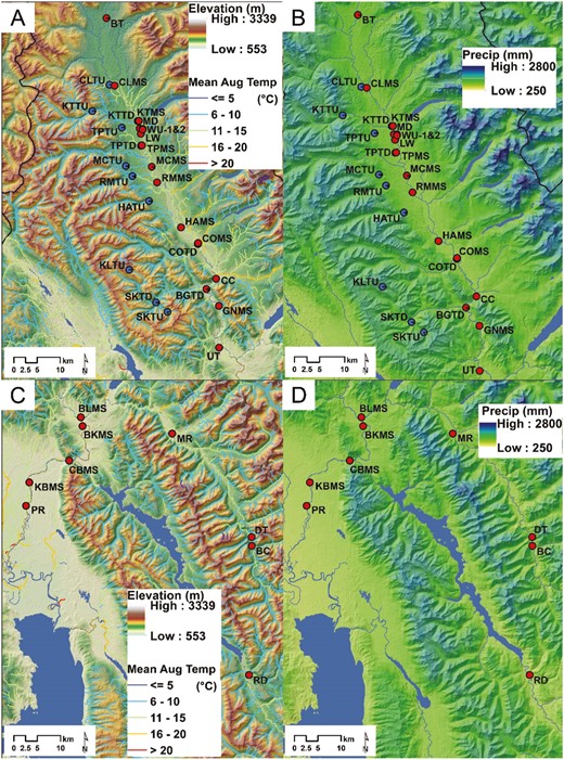
Maps of environmental layers (A and C) Elevation and Temperature, and (B and D) Precipitation for sites on the (A and B) North Fork of the Flathead and (C and D) sites on the mainstem Flathead, Middle Fork, and South Forks of the Flathead River. (Red = Sweltsa coloradensis and blue = Sweltsa fidelis. Sites in the Elk River (MC, SP) and PO are not shown to improve view of the majority of the sites. Sites containing unidentified Sweltsa spp (UNKNOWN1) individuals include: SKTD, SKTU, RMTU, MCTU, KTTD, PO, BGTD, COTD, COTU, MCPO, EL.
Cold-Water Habitat Patchiness, Dispersal, and Structure
It is well known that temperature is the strongest controller of stonefly distributions. Generally, temperature decreases with elevation, but this relationship is complicated by the presence of cold-water spring habitats for S. fidelis at varying elevations. However, springs were not sampled in this study. A patchwork of cold-water habitats and substantial dispersal by long-winged S. fidelis could facilitate higher than expected gene flow for the population at large and thereby help explain the lack of population structure within the North Fork of the Flathead drainages. Better than expected dispersal abilities and anomalies in distribution of S. fidelis with respect to elevation may also explain why the genetic structure of S. fidelis was not well described by environmental variables, although fewer sampling sites and lower statistical power might also explain it.
Conclusions
Our results suggest similarly weak population genetic subdivision and high connectivity among sampling locations within both the mainstem and tributary stonefly species. This finding is consistent with previous research suggesting that flight at the adult stage promotes population connectivity, even in species like stoneflies that are considered to have poor dispersal. Our results also provide correlative evidence that climate-related variables can influence adaptive genetic variation. Further, this study demonstrates that general understanding of the environmental drivers of genetic diversity can be improved when studying both neutral and adaptive variation in closely related species with limited geographic overlap and distinct habitats. Future research should further address the relationship between gene flow and environmental variables (e.g., time-series data with warming waters, changing hydrology, precipitation, etc.) in order to model the effects of climate change. Future research could include higher density loci (e.g., whole genome resequencing) for higher power to detect adaptive genetic variation.
Funding
This work was funded by a National Science Foundation Dimensions of Biodiversity Grant #DOB-1639014 and approved under a Forest Service Special Use Permit.
Acknowledgments
We thank the Dalimata family for allowing us to conduct a portion of this research on their land and for helping with field support. We thank field crew members for assistance with sample collection: Garrett Frandson, Hailey Jacobson, Megan Ritter, Wesley Sigl, and Keridwen Whitmore. We thank Brenna Forester for her help and input on GEAs and RDA tests. Any use of trade, firm, or product names is for descriptive purposes only and does not imply endorsement by the US Government.
Data Availability
Sampling locations and environmental data have been published online: https://doi.org/10.5061/dryad.5x69p8d5w.
DNA sequences have been uploaded to GenBank.
Data Accessibility
All associated genetic data for the resources detailed in this study, including both raw reads and assembly, are available as part of GenBank BioProject PRJNA843028. All environmental data have been published online: https://doi.org/10.5061/dryad.5x69p8d5w.
References
Author notes
Shared first authorship. These authors contributed equally to the work.
