


Abstract
With the advent of next-generation sequencing approaches, the search for individual loci underlying local adaptation has become a major enterprise in evolutionary biology. One promising method to identify such loci is to examine genome-wide patterns of differentiation, using an FST-outlier approach. The effects of pleiotropy and epistasis on this approach are not yet known. Here, we model 2 populations of a sexually reproducing, diploid organism with 2 quantitative traits, one of which is involved in local adaptation. We consider genetic architectures with and without pleiotropy and epistasis. We also model neutral marker loci on an explicit genetic map as the 2 populations diverge and apply FST outlier approaches to determine the extent to which quantitative trait loci (QTL) are detectable. Our results show, under a wide range of conditions, that only a small number of QTL are typically responsible for most of the trait divergence between populations, even when inheritance is highly polygenic. We find that the loci making the largest contributions to trait divergence tend to be detectable outliers. These loci also make the largest contributions to within-population genetic variance. The addition of pleiotropy reduces the extent to which quantitative traits can evolve independently but does not reduce the efficacy of outlier scans. The addition of epistasis, however, reduces the mean FST values for causative QTL, making these loci more difficult, but not impossible, to detect in outlier scans.
Recent advances in genomics have spurred a search for individual loci involved in local adaptation (Stapley et al. 2010; Feder et al. 2012; Hoban et al. 2016; Ahrens et al. 2018). The identification of such loci promises to shed additional light on the relationship between local selection pressures and gene flow in shaping patterns of variation across species’ ranges (Hohenlohe et al. 2010; Savolainen et al. 2013). In general, loci involved in adaptation are expected to be polymorphic and to display substantial differences in allele frequencies across populations. The allele frequency differences are caused by selection, driven by spatial variation in the fitness effects of individual alleles (Williams 1966; Kawecki and Ebert 2004). In other words, a given allele may be adaptive in one environment but deleterious in a different environment. Consequently, variation at such loci is governed by a balance between migration and selection, leading to an expectation that differences in allele frequencies among populations should be greater than those expected for neutral loci (Cavalli-Sforza 1966; Lewontin and Krakauer 1973).
The search for adaptive loci in nature may be more difficult than it initially appears because the phenotypes involved in adaptation are often quantitative traits (or complex traits), determined by allelic effects at many loci as well as environmental effects (Falconer and Mackay 1996; Brady et al. 2005). Some examples of adaptive single-gene traits have been identified (Kohn et al. 2003; Storz and Dubach 2004), but most evidence suggests that polygenic traits are the most common targets of adaptive divergence in nature (Pritchard et al. 2010; Gagnaire et al. 2013; Sork 2017). This situation is especially unnerving because genetic variation in complex traits may be determined by dozens, hundreds, or thousands of loci spread across the genome (Flint and Mackay 2009; Yang et al. 2010; Boyle et al. 2017). Moreover, the genetic architecture of a typical quantitative trait may include substantial nonadditive effects, such as dominance and epistasis (Phillips 2008; Hendry 2013; Mackay 2014). These considerations point to a need for improved methods to detect adaptive loci associated with complex trait variation in nature.
A growing body of work has begun to address the efficacy of various approaches to genome-wide scans for adaptive loci in a population genomics context (Storz 2005; Pérez-Figueroa et al. 2010; Narum and Hess 2011; Vilas et al. 2012; De Mita et al. 2013; Jones et al. 2013; De Villemereuil et al. 2014; Lotterhos and Whitlock 2014, 2015; Frichot et al. 2015; Yoder and Tiffin 2017). A common approach is to simulate datasets under various demographic scenarios and analyze them using a variety of techniques. These studies can be extremely illuminating, as they often reveal hidden pitfalls and limitations of population genomic methods. For instance, a series of articles by Lotterhos and Whitlock (2014, 2015) has contributed to a deeper understanding of how scans for outlier loci and genotype–environment associations are affected by demographic factors and sampling schemes (Lottherhos and Whitlock 2014, 2015). These insights have contributed directly to the development of refined methods for the detection of adaptive loci (Whitlock and Lotterhos 2015; Verity et al. 2017).
A current limitation of simulation-based studies of the efficacy of genome-wide scans is that they use very simple genetic architectures for the traits under consideration. Lotterhos and Whitlock (2014, 2015), for instance, assume that selection is applied equally to a specified number of loci involved in local adaptation, thus sidestepping the issue that, in nature, the loci under selection are usually quantitative trait loci (QTL), with the associated quantitative traits serving as the actual targets of selection. Thus, selection on individual loci may be more diffuse and variable than the situations modeled by Lotterhos and Whitlock (2014, 2015). Other studies have modeled more realistic quantitative genetic architectures in the context of local adaptation (Vilas et al. 2012), but even these studies have not progressed beyond a strictly additive model, even though pleiotropy and epistasis are nearly universal features of the genetic architecture of all but the simplest of traits (Mackay 2014; Shorter et al. 2015). Furthermore, recent perspectives on the detection of loci involved in local adaptation have specifically pinpointed pleiotropy and epistasis as areas of need for additional work (Hoban et al. 2016; Csilléry et al. 2018).
In the present study, we use a simulation-based approach to investigate how quantitative genetic architectures that include pleiotropy and epistasis affect patterns of differentiation and consequently the efficacy of genome-wide scans for selection based on outlier loci. Here, we model the evolution of 2 quantitative traits in a pair of populations linked by migration. We examine the extent to which pleiotropy and epistasis affect the ability of the populations to adapt to their local optima. We also investigate the dynamics of differentiation at marker loci and quantitative trait loci arranged on explicitly modeled linkage groups. These simulations permit us to examine how pleiotropy and epistasis affect the potential for genome scans to detect outlier loci associated with trait divergence among populations.
Methods
We use an individual-based, forward-in-time simulation to explicitly model 2 populations linked by migration. Our simulation is based on the multivariate models developed by Jones et al. (2003, 2004, 2007, 2012, 2014) to study the genetic architecture of quantitative traits and the evolution of the mutational matrix in evolving populations. These models explicitly simulate every individual in a population of a diploid organism with separate sexes. For the current study, the main additions to the model, which are described in more detail below, include an expansion to 2 populations connected by migration, explicit modeling of linkage groups with recombination and neutral marker loci, and the ability to specify loci with and without pleiotropic and epistatic effects.
The Genetic System
The simulation model specifies a genome containing neutral marker loci and quantitative trait loci affecting 2 quantitative traits. The marker loci are arranged on linkage groups, each of which has a specified recombination rate. In this study, we allow each marker locus to have up to 4 alleles, and they are evenly spaced along linkage groups. Thus, the markers can be interpreted as resulting from an exon-capture approach, a filtered RAD-seq dataset, or any other method that ensures a reasonably even representation of markers across the genome. The simulation framework can accommodate many thousands of marker loci. In the present study, we usually simulate 8000 marker loci on 4 linkage groups but also consider cases with up to 40 000 loci. A mutation at a marker locus results in a random change to one of the other possible allelic states, and all possible changes are equally likely.
We model 2 quantitative traits, determined by a specified number of quantitative trait loci (see Table 1 for parameters and symbols). The quantitative trait loci are randomly placed on linkage groups, and each quantitative trait locus is assumed to be in the immediate vicinity of a single marker locus, which may or may not be polymorphic during an actual simulation run. In the absence of epistasis, an individual’s genetic value for a trait is determined by summing across the quantitative trait loci corresponding to the trait in question. The model can include loci that affect only trait 1, loci that affect only trait 2, and pleiotropic loci that affect both traits. For loci affecting a single trait, mutational effects are drawn from a normal distribution with a mean of 0 and variance of α11 or α22. For pleiotropic loci, which have allelic effects on both traits, mutational effects are drawn from a bivariate normal distribution with means of 0, variances of α11 and α22, and a covariance of α12. Mutational effects are added to the existing allelic effects, adhering to the continuum-of-alleles model (Crow and Kimura 1964).
Parameters used in the model and their values in the core parameter set
| Parameter | Symbol | Typical value | Explanation |
|---|---|---|---|
| Population size | N | 500 | The current number of adults in the population |
| Carrying capacity | K | 500 | The number of adults is randomly culled to this number before reproduction (but after selection) each generation |
| Female fecundity | 2B | 4 | Number of offspring produced per female |
| Migration rate | m | 0.016 | The proportion of juveniles in a population that originated from the other population |
| Sample size | S | 100 | The size of the simulated sample of adults used for genotyping per population |
| Number of linkage groups | nL | 4 | The number of linkage groups (chromosomes) onto which the marker loci and QTL are placed |
| Recombination rate per linkage group | R | 0.25 | The expected number of recombination events per linkage group per meiosis during the production of gametes |
| Number of QTL per linkage group | nq1, nq2, nqP | 1 | The number of QTL per linkage group. The QTL fall into 3 categories: those affecting trait 1 (nq1), those affecting trait 2 (nq2), and those that are pleiotropic (nqP). |
| Number of marker loci per linkage group | nm | 2000 | The number of neutral marker loci (e.g., single nucleotide polymorphisms) per linkage group |
| Marker mutation rate | μm | 0.0002 | The probability per allele per meiosis of a mutation at a marker locus |
| QTL mutation rate | μq | 0.0002 | The probability per allele per meiosis of a mutation at a QTL |
| Mutational variances | α11, α22 | 0.2 | The variance of the Gaussian distribution (with mean 0) from which new allelic effects are drawn for the 2 traits when a mutation occurs. This allelic effect is added to an allele’s existing effect. |
| Mutational covariance | α12 | 0 | The covariance of a bivariate normal distribution (with means 0) from which allelic effects are drawn when a mutation occurs at a pleiotropic locus |
| Environmental variance | 1 | The variance of the normal distribution, with mean 0, from which environmental effects are drawn. These effects are added to an individual’s breeding value to determine the phenotype. | |
| Variance in epistatic parameters | 0, 1.6 | The variance of the normal distribution, with mean 0, from which epistatic parameters are drawn. Larger values result in epistatic parameters with larger absolute effects on average. | |
| Trait optima | θ1, θ2 | 4, −4 | The position of the optimum for each trait. Each population has a value of θ1 (the trait 1 optimum) and θ2 (the trait 2 optimum), and these values can differ between populations. |
| Elements of the ω-matrix | ω11, ω22, ω12 | 49, 49, 0 | The ω-matrix specifies the steepness and orientation of the individual selection surface. Lower values result in stronger selection (toward the optimum), and ω12 determines the strength of correlational selection. |
We model epistasis using the multilinear model of Hansen and Wagner (2001), extended to a multivariate phenotype, as described by Jones et al. (2014). Many types of epistasis can be represented using the multilinear model, which extends a strictly additive model by adding a series of terms corresponding to the effects of interactions among loci. In a strictly additive model, an individual’s genotypic value (i.e., breeding value) for a trait is determined by summing across alleles and loci (Falconer and Mackay 1996; Lynch and Walsh 1998). In the univariate multilinear model, an individual’s genotypic value (X) for a trait is given by
where ξ0 is an arbitrary reference genotype, which we assume to be 0, y(i) is the reference effect of an individual’s genotype at locus i, and ε(i, j) is an epistatic coefficient determining the strength of the interaction between locus i and locus j. This formulation reduces to a simple additive model when all epistatic coefficients are set to 0, and the reference effects can then be interpreted as additive effects. In the presence of epistasis, reference effects cannot be interpreted simply as additive effects because the epistatic terms also contribute to the additive genetic variance.
In the presence of multiple traits, the model becomes somewhat more complex, because now interactions between allelic effects at different traits also become possible (Jones et al. 2014). For instance, if we allow universal pleiotropy in a 2-trait system, such that every locus has an allelic effect for both traits, then an individual’s genotypic value is specified as
where aX is the individual’s genotypic value for trait a, aξ0 is the trait a reference genotype (assumed here to be 0), ay(i) is the reference effect of locus i on trait a, and abcε(i, j) is the epistatic coefficient describing the effects on trait a of the interaction between the locus i reference effect on trait b and the locus j reference effect on trait c. No locus interacts with itself, so abcε(i, i) = 0, and interactions are symmetric, such that abcε(i, j) = acbε(j, i). The multilinear model for nonpleiotropic loci, which we also investigate here, is slightly simplified in the sense that each locus has a reference effect only on a single trait. However, we still allow between-trait epistatic effects. That is, a trait 1 locus can interact with a trait 2 locus and produce an effect on either trait.
The multilinear model requires a large number of epistatic parameters. The 2-trait, pleiotropic model, for instance, requires a total of 4nqP(nqP − 1) epistatic coefficients, where nqP is the number of pleiotropic quantitative trait loci. Thus, a model with 2 such loci would require only 8 epistatic parameters, whereas a model with 20 epistatic, pleiotropic quantitative trait loci would require a whopping 1520 epistatic parameters. Given their large number, we draw these epistatic parameters from a Gaussian distribution with a mean of 0 and a variance of . Thus, larger values of result in larger absolute epistatic effects on average, though positive and negative epistatic effects are equally likely. These epistatic parameters are drawn randomly at the beginning of a simulation run, are identical in both populations, and remain invariant during the run. Thus, epistatic effects in the multilinear model evolve as a consequence of the evolution of reference effects, not due to changes in the epistatic coefficients.
After each individual’s genotypic values are tallied, we simulate environmental variance by adding a random number drawn from a Gaussian distribution with mean 0 and variance to the genotypic value for each trait to produce a corresponding phenotypic value for each trait. Environmental effects are assumed to be independent across traits.
The Life Cycle
Our model simulates a population of a diploid, sexually reproducing species with separate sexes. The mating system is polygynous. Each female chooses a male at random and produces 2B offspring with him. Males have no limit to the number of times they can mate or the number of offspring they can produce.
Markers and quantitative trait loci are explicitly placed on linkage groups, which can be thought of as chromosomes or regions of chromosomes, and recombination events occur during a simulated meiosis. The mean number of recombination events per linkage group is determined by the parameter R, and the actual number for each chromosome is drawn from a Poisson distribution. Mutations are also allowed to occur during this meiosis phase, and their effects are described above. For each linkage group, we generate an expected number of mutations by drawing a random number from a Poisson distribution with a mean equal to the number of loci times the mutation rate. We then choose this number of loci at random on which to impose a mutation. This approach simply saves computational time, as testing for mutations on a locus-by-locus basis would require thousands of random numbers per generation. The linkage groups from the chosen mother and father, after mutation and recombination, are united to form a zygote with a full complement of diploid loci.
Natural selection is imposed as viability selection during development from zygote to adulthood. We use a standard individual selection surface, which has a Gaussian shape, such that an individual’s fitness is given by
where z is a vector of phenotypic values for the traits of interest, θi is a vector of trait optima in population i, and ω is a matrix describing the selection surface. In the bivariate case, ω is a symmetric matrix whose diagonal elements describe the strength of stabilizing selection on traits 1 and 2, whereas the off-diagonal element describes the strength of correlational selection. For the results shown here, ω is assumed to be the same in both demes. We generally use values of 49 for ω11 and ω22, which represents stabilizing selection near the weaker end of empirical estimates (Kingsolver et al. 2001). Directional selection occurs whenever the population mean is displaced from the optimum. We treat W(z) as the probability that an individual survives viability selection by drawing a uniformly distributed number ranging from 0 to 1. If the random number is less than W(z), then the individual survives selection.
The survivors of selection are subject to population regulation. We impose a carrying capacity of K. If fewer than K individuals survive selection, then they are all retained as adults in the population. If more than K individuals survive selection, then individuals are culled at random until K individuals remain. For most simulations, we use a K of 500, and the adult population size typically remains at the carrying capacity for the duration of the simulation run. After population regulation, we have a new population of adults and the lifecycle begins again with random mating.
Migration
In the present study, we simulate 2 populations linked by migration. Migration is symmetric and occurs after the production of progeny but before natural selection. Hence, juveniles migrate in our model. The number of migrants is determined as the product of the migration rate and the number of progeny present in each population. Any fractions are treated as a probability of adding an additional migrant. For example, if the expected number of migrants for a given generation is 4.3, then the number of migrants would be 4 with probability 0.7 and 5 with probability 0.3. These probabilities are resolved by drawing a random number from a uniform distribution between 0 and 1. Once the number of migrants is determined, the 2 populations simply exchange this number of individuals.
Running the Simulations
Each simulation run starts with 2 populations of adults, initialized with 4 equally frequent alleles at each marker locus. Each quantitative trait locus is also initialized with 4 equally frequent alleles, with allelic effects drawn from a Gaussian distribution with a standard deviation of 0.05. Initially, markers and quantitative trait loci are in complete linkage disequilibrium within a linkage group (so the population starts with 4 versions of each linkage group, resulting in 10 possible diploid genotypes per linkage group in the initial population).
The simulation begins with 10 000 initial generations, during which the 2 populations evolve under the same bivariate optimum, arbitrarily chosen to be 0 for each trait. During this period, the 2 populations are linked by mutation, and they achieve a mutation-drift-migration-selection balance. Linkage disequilibrium also breaks down due to recombination. After these initial generations, each population’s bivariate optimum is changed to a desired value to reflect habitat differences. In most cases, we move only the trait 1 optima. We choose values of the trait optima that allow substantial differentiation without making population persistence unlikely. We use a difference of 8 units of trait 1 (i.e., an optimum of 4 in population 1 and −4 in population 2), resulting in divergence of more than 7 phenotypic standard deviations in the absence of migration. In this class of model, the scale is often set by the environmental standard deviation (Jones et al. 2003, 2004), which we set at 1 in the present study. Thus, 8 units of trait 1 is also 8 environmental standard deviations. Investigations involving different positions of the optima indicate that these values provide a favorable case for the detection of outliers by imposing strong selection on QTL without seriously limiting the ability of individuals to survive migration between populations.
Another 2000 generations are imposed, after the initial stabilizing selection generations, to allow the populations to equilibrate to the new optima. Finally, these generations are followed by 2000 experimental generations, during which we calculate summary statistics of interest. See Table 1 for a list of important parameters of the model and their typical values in simulation runs. Most simulations start from this core parameter value set and systematically vary one parameter to isolate its effects on the system.
Each combination of parameter values is usually replicated in 30 independent simulation runs. Each simulation run has a new set of starting allelic values, randomly chosen epistatic parameters, and locations of the quantitative trait loci on linkage groups.
Calculating Variables of Interest
We calculate a number of variables of interest related to the efficacy of local adaptation and the ability of genome-wide scans to detect outlier loci. With respect to quantitative genetic variables, we compile data regarding the phenotypic mean, phenotypic variances and covariance, total genetic variances and covariance, and additive genetic variances and covariance. These values are averaged across experimental generations.
We also calculate per-locus values of FST for marker loci and quantitative trait loci. These values are calculated from a simulated sample of adults drawn from the 2 populations. Typically, we assume a sample size of 100 individuals per population. We use the formula FST = (HT − HS)/HT, where HT is the total expected heterozygosity (i.e., when populations are lumped) and HS is the mean within-population expected heterozygosity. This formula ensures that all FST values are positive, which is a necessary prerequisite for our chosen method of detecting outliers (Whitlock and Lotterhos 2015), while still being highly correlated with more complex formulas for FST estimation.
We take 2 approaches for the detection of FST outliers among our marker loci. First, we use the method of Whitlock and Lotterhos (2015), which is an implementation of the approach originally suggested by Lewontin and Krakauer (1973). This method is based on the observation that, for a given locus, the value
is expected to have a χ2 distribution with npops − 1 degrees of freedom. Whitlock and Lotterhos (2015) improve upon the Lewontin and Krakauer (1973) approach by introducing an iterative method to estimate the degrees of freedom from the core of the distribution, thus reducing the bias introduced by outlier loci. However, our implementation, which requires hard-coding into our simulations, assumes npops − 1 = 2 − 1 = 1 degree of freedom. This assumption will make our P values slightly less accurate than those that would be produced by the Whitlock and Lotterhos (2015) approach.
We supplement the Whitlock and Lotterhos (2015) approach for outlier detection by using smoothed FST values and calculating arbitrary confidence intervals based on the mean and standard deviations of the smoothed values. We calculate smoothed values according to the sliding window approach used by Hohenlohe et al. (2010), where values are weighted according to a Gaussian function. We use a variance of 500 marker positions for this procedure. We then calculate 99% and 95% confidence intervals as and , respectively, where is the mean smoothed FST value for the linkage group and is the standard deviation in smoothed FST values for the linkage group. Marker loci with FST values above the critical values were considered outliers at either 99% or 95% confidence. These critical values were calculated separately for each linkage group, whereas the Whitlock and Lotterhos (2015) approach was applied genome-wide.
All tests for outlier loci in this study focus on marker loci, not the quantitative trait loci themselves, as we are assuming that the loci underlying phenotypic traits are not known. We also restrict attention to marker loci that are near a smoothed FST peak, for both the Whitlock and Lotterhos (2015) and smoothed FST approaches. Even though all tests for outliers focus on the marker loci, we do calculate FST values for quantitative trait loci for comparison. We conduct our outlier tests on the final experimental generation of each simulation run.
Results
Evolution of Local Adaptation
As expected, this model produces a migration-selection balance when the 2 evolving populations have different optima. In this study, we hold the optimum for trait 2 constant at 0, while imposing separate trait 1 optima for the 2 populations. Under most circumstances, we use a trait 1 optimum of 4 for population 1 and an optimum of −4 for population 2. In the absence of migration, the difference between optima represents about 7 phenotypic standard deviations, which is large enough to produce meaningful divergence, without imposing too large a cost as the populations evolve from their initial optima of 0 to their experimental optima of 4 or −4. Investigation of other differences between optima, ranging from 2 to 20, produces similar qualitative results to those presented in this report.
Table 2 shows some important results regarding trait means and genetic variances when QTL are not pleiotropic, and the trait optima are set to 4 in population 1 and −4 in population 2. The top half of the table shows results without epistasis (i.e., = 0). When the migration rate is 0, of course, the populations independently evolve trait means very close to their optima (Table 2, first row). As the migration rate increases, each population finds its mean for trait 1 displaced from the relevant optimum by migration. In the extreme case of m = 0.256, which means that approximately a quarter of individuals in each population originated from the other population each generation, population means for each population end up very close to 0, the midpoint between the 2 optima. Because the positions of the population means are determined by a balance between selection and migration, either weaker selection or a smaller difference in optima between the 2 populations would result in population means closer to the midpoint in optima between populations.
The evolution of local adaptation and the genetic architecture in 2 populations with different trait optima, assuming no pleiotropy
| Population 1 | Population 2 | |||||||||||
|---|---|---|---|---|---|---|---|---|---|---|---|---|
| m | ||||||||||||
| 0 | 0 | 4.01 (0.04) | −0.05 (0.04) | 0.102 (0.011) | 0.099 (0.010) | 0.000 (0.000) | −3.95 (0.04) | 0.05 (0.04) | 0.101 (0.012) | 0.084 (0.010) | 0.000 (0.000) | |
| 0.002 | 0 | 3.69 (0.03) | 0.00 (0.03) | 0.597 (0.024) | 0.101 (0.009) | −0.001 (0.002) | −3.77 (0.03) | 0.01 (0.03) | 0.682 (0.030) | 0.103 (0.010) | −0.001 (0.001) | |
| 0.004 | 0 | 3.67 (0.03) | 0.02 (0.03) | 1.109 (0.041) | 0.104 (0.011) | 0.000 (0.001) | −3.68 (0.03) | 0.03 (0.02) | 1.124 (0.041) | 0.096 (0.011) | 0.000 (0.001) | |
| 0.008 | 0 | 3.52 (0.03) | −0.01 (0.02) | 1.903 (0.047) | 0.106 (0.007) | 0.001 (0.002) | −3.51 (0.02) | −0.02 (0.02) | 1.865 (0.051) | 0.106 (0.007) | 0.000 (0.002) | |
| 0.016 | 0 | 3.24 (0.03) | 0.00 (0.02) | 3.108 (0.083) | 0.105 (0.083) | −0.005 (0.002) | −3.22 (0.03) | 0.01 (0.03) | 3.062 (0.079) | 0.106 (0.010) | −0.004 (0.002) | |
| 0.032 | 0 | 2.81 (0.02) | 0.00 (0.02) | 4.761 (0.107) | 0.108 (0.011) | −0.002 (0.002) | −2.78 (0.03) | 0.01 (0.02) | 4.689 (0.108) | 0.111 (0.011) | −0.001 (0.002) | |
| 0.064 | 0 | 2.02 (0.04) | 0.04 (0.03) | 6.075 (0.149) | 0.118 (0.010) | −0.001 (0.002) | −2.01 (0.03) | 0.04 (0.03) | 6.045 (0.137) | 0.116 (0.010) | 0.000 (0.002) | |
| 0.128 | 0 | 0.79 (0.03) | −0.02 (0.02) | 4.348 (0.215) | 0.107 (0.010) | −0.004 (0.002) | −0.80 (0.04) | −0.02 (0.02) | 4.421 (0.228) | 0.108 (0.010) | −0.005 (0.002) | |
| 0.256 | 0 | 0.03 (0.02) | 0.00 (0.02) | 0.322 (0.042) | 0.109 (0.007) | −0.001 (0.001) | −0.02 (0.02) | 0.00 (0.02) | 0.323 (0.042) | 0.109 (0.007) | −0.001 (0.001) | |
| 0 | 1.6 | 3.95 (0.04) | 0.00 (0.06) | 0.189 (0.015) | 0.137 (0.011) | 0.001 (0.008) | −4.01 (0.05) | −0.08 (0.05) | 0.162 (0.011) | 0.163 (0.022) | 0.000 (0.011) | |
| 0.002 | 1.6 | 3.88 (0.05) | −0.07 (0.04) | 0.699 (0.046) | 0.285 (0.034) | −0.010 (0.034) | −3.82 (0.05) | −0.01 (0.04) | 0.667 (0.033) | 0.279 (0.031) | 0.002 (0.014) | |
| 0.004 | 1.6 | 3.76 (0.05) | −0.09 (0.05) | 1.166 (0.053) | 0.382 (0.043) | −0.014 (0.034) | −3.66 (0.04) | 0.08 (0.05) | 1.065 (0.046) | 0.411 (0.037) | −0.060 (0.031) | |
| 0.008 | 1.6 | 3.58 (0.04) | 0.04 (0.05) | 1.797 (0.083) | 0.440 (0.056) | 0.012 (0.036) | −3.59 (0.04) | 0.10 (0.05) | 1.798 (0.066) | 0.359 (0.045) | 0.005 (0.039) | |
| 0.016 | 1.6 | 3.27 (0.05) | −0.05 (0.05) | 2.707 (0.063) | 0.392 (0.072) | 0.005 (0.066) | −3.23 (0.04) | 0.07 (0.06) | 2.771 (0.108) | 0.397 (0.059) | −0.105 (0.064) | |
| 0.032 | 1.6 | 2.84 (0.06) | −0.03 (0.06) | 4.557 (0.135) | 0.439 (0.061) | −0.135 (0.072) | −2.80 (0.06) | 0.12 (0.05) | 4.347 (0.130) | 0.466 (0.079) | −0.132 (0.084) | |
| 0.064 | 1.6 | 2.12 (0.04) | 0.16 (0.04) | 6.144 (0.153) | 0.345 (0.050) | 0.161 (0.087) | −2.07 (0.05) | 0.02 (0.05) | 6.070 (0.169) | 0.341 (0.046) | 0.202 (0.085) | |
| 0.128 | 1.6 | 0.58 (0.05) | 0.05 (0.03) | 3.334 (0.273) | 0.325 (0.024) | −0.032 (0.071) | −0.60 (0.05) | 0.06 (0.04) | 3.354 (0.258) | 0.330 (0.027) | 0.008 (0.076) | |
| 0.256 | 1.6 | 0.00 (0.03) | 0.00 (0.03) | 0.191 (0.019) | 0.117 (0.008) | −0.002 (0.006) | −0.03 (0.03) | 0.00 (0.03) | 0.191 (0.020) | 0.117 (0.008) | −0.002 (0.006) |
These simulations used the core set of parameter values (Table 1). Each quantitative trait was determined by 4 quantitative trait loci, and these loci were not pleiotropic (i.e., each of the 2 traits was determined by an independent set of loci). The genome consisted of 4 linkage groups, with 1 QTL per trait per linkage group. The epistatic variance () indicates the variance of the normal distribution from which epistatic parameters were drawn, with a value of 0 indicating no epistatic effects. The 2 simulated populations differed with respect to the location of the bivariate optimum. The optimum for trait 1 in population 1 had a value of 4, whereas the trait 1 optimum in population 2 had a value of −4. Both populations had an optimum of 0 for trait 2. This table shows the migration rate (m), the aforementioned epistatic variance (), the means of the 2 traits ( and ), and the total genetic variances and covariance for the 2 traits (, , and ) for each of the 2 populations. Each value is a mean across 30 independent simulations, with the standard error of these means shown in parentheses.
In the absence of epistasis (Table 2, top half), the genetic variance for trait 1 is strongly affected by migration (11VG). As the migration rate increases from 0 to 0.064, we see a 60-fold increase in genetic variance (in the absence of epistasis, all of this genetic variance is additive). This increase is due to the migration of alleles with strikingly different average allelic effects from the other population (Guillaume and Whitlock 2007; Yeaman and Whitlock 2011). The genetic variance for trait 2 (22VG) and the genetic covariance (12VG) are only slightly affected by migration. These small effects are probably due to occasional linkage disequilibrium between QTL for the 2 traits.
When the migration rate becomes extremely large, we begin to see a decrease in the trait 1 genetic variance (Table 2, m = 0.128, m = 0.256). This effect occurs because the populations are so well mixed that they are beginning to behave as a single panmictic population spanning a 2-peaked selection surface. This feature is most evident when m = 0.256. In this case, both population means for trait 1 are near 0, and the additive genetic variance is about 20-fold lower than it is for m = 0.064. However, the genetic variance is still about 3-fold higher than it is in the absence of migration, consistent with a population experiencing the disruptive selection that would be expected from a 2-peaked selection surface.
In the presence of epistasis (Table 2, bottom half), the evolution of local adaptation closely mirrors the patterns seen in the absence of epistasis. While some small, quantitative differences are apparent, the overall pattern is similar, and epistasis shows no universal tendencies to facilitate or retard local adaptation. Even the total genetic variance for trait 1 shows almost the same pattern whether or not epistasis is part of the genetic architecture (Table 2, 11VG). Interestingly, even with epistasis, almost all of the genetic variance for trait 1 is additive genetic variance. This result may stem partially from our use of nondirectional epistasis (i.e., a mean of 0 for our distribution of epistatic parameters), but is also due to large differences in reference effects between populations at some loci (see below). The most striking difference between genetic architectures with and without epistasis concerns the genetic variance of the second trait. In the presence of epistasis, we see a larger increase in the genetic variance of trait 2 as the genetic variance of trait 1 increases (Table 2, 22VG), in comparison to genetic architectures lacking epistasis. This pattern stems from the epistatic interactions between QTL for the 2 traits, which restrict the extent to which the traits can evolve independently. We also see a tendency for the genetic covariances to be more variable (cf. the SEM values for 12VG with and without epistasis) in the presence of epistasis, another effect that is attributable to the between-trait epistatic interactions. Thus, with epistasis, populations sometime evolve genetic covariances that differ more from 0 (either in a positive or negative direction) than those that evolve without epistasis and pleiotropy.
Table 3 shows results for the evolution of the trait means and genetic variances when all QTL are pleiotropic, with and without epistasis. Interestingly, nearly all of the patterns observed in the absence of pleiotropy also occur in the presence of pleiotropy. The only notable and expected exception is that with pleiotropy, even in the absence of epistasis, factors affecting the genetic variance for trait 1 also impact the genetic variance for trait 2, as a direct consequence of pleiotropy.
Local adaptation and the evolution of the genetic architecture when all loci are pleiotropic, with and without epistasis
| Population 1 | Population 2 | |||||||||||
|---|---|---|---|---|---|---|---|---|---|---|---|---|
| m | ||||||||||||
| 0 | 0 | 4.00 (0.06) | 0.00 (0.05) | 0.084 (0.013) | 0.077 (0.008) | 0.003 (0.006) | −3.94 (0.06) | 0.02 (0.06) | 0.114 (0.015) | 0.102 (0.012) | 0.006 (0.012) | |
| 0.002 | 0 | 3.82 (0.04) | 0.00 (0.05) | 0.684 (0.035) | 0.146 (0.014) | −0.017 (0.012) | −3.75 (0.04) | 0.07 (0.06) | 0.649 (0.025) | 0.144 (0.014) | −0.019 (0.012) | |
| 0.004 | 0 | 3.69 (0.03) | 0.04 (0.05) | 0.982 (0.027) | 0.182 (0.018) | 0.023 (0.018) | −3.66 (0.03) | 0.00 (0.04) | 1.034 (0.044) | 0.184 (0.019) | −0.001 (0.011) | |
| 0.008 | 0 | 3.43 (0.03) | −0.04 (0.04) | 1.748 (0.065) | 0.235 (0.22) | −0.020 (0.019) | −3.40 (0.03) | −0.01 (0.05) | 1.683 (0.054) | 0.249 (0.029) | −0.025 (0.022) | |
| 0.016 | 0 | 3.23 (0.03) | −0.07 (0.05) | 3.000 (0.078) | 0.246 (0.030) | −0.060 (0.035) | −3.18 (0.04) | 0.09 (0.05) | 2.883 (0.070) | 0.258 (0.037) | −0.091 (0.044) | |
| 0.032 | 0 | 2.69 (0.03) | −0.01 (0.04) | 4.403 (0.101) | 0.240 (0.031) | 0.019 (0.043) | −2.70 (0.03) | −0.02 (0.04) | 4.504 (0.118) | 0.253 (0.030) | 0.018 (0.046) | |
| 0.064 | 0 | 1.88 (0.04) | −0.05 (0.04) | 5.451 (0.193) | 0.267 (0.026) | −0.014 (0.097) | −1.90 (0.04) | −0.04 (0.04) | 5.578 (0.181) | 0.273 (0.025) | −0.007 (0.100) | |
| 0.128 | 0 | 0.59 (0.05) | −0.05 (0.03) | 3.176 (0.259) | 0.245 (0.031) | −0.268 (0.062) | −0.61 (0.04) | 0.05 (0.03) | 3.137 (0.237) | 0.245 (0.032) | −0.251 (0.059) | |
| 0.256 | 0 | −0.01 (0.02) | 0.00 (0.02) | 0.192 (0.028) | 0.097 (0.009) | 0.001 (0.008) | −0.03 (0.02) | 0.00 (0.02) | 0.193 (0.027) | 0.097 (0.009) | 0.000 (0.008) | |
| 0 | 1.6 | 3.91 (0.08) | 0.02 (0.06) | 0.144 (0.023) | 0.131 (0.039) | −0.002 (0.007) | −4.02 (0.07) | 0.04 (0.08) | 0.162 (0.038) | 0.109 (0.017) | −0.017 (0.019) | |
| 0.002 | 1.6 | 3.81 (0.06) | 0.09 (0.06) | 0.636 (0.049) | 0.301 (0.041) | −0.009 (0.023) | −3.85 (0.05) | −0.06 (0.06) | 0.678 (0.058) | 0.266 (0.043) | 0.033 (0.022) | |
| 0.004 | 1.6 | 3.68 (0.05) | −0.08 (0.06) | 1.071 (0.081) | 0.405 (0.073) | 0.009 (0.043) | −3.64 (0.06) | 0.08 (0.08) | 1.030 (0.048) | 0.332 (0.037) | −0.009 (0.035) | |
| 0.008 | 1.6 | 3.65 (0.06) | 0.07 (0.06) | 1.868 (0.089) | 0.479 (0.061) | 0.043 (0.061) | −3.58 (0.06) | −0.11 (0.08) | 1.913 (0.093) | 0.418 (0.054) | −0.020 (0.059) | |
| 0.016 | 1.6 | 3.35 (0.07) | 0.07 (0.08) | 2.817 (0.135) | 0.443 (0.077) | 0.080 (0.057) | −3.32 (0.07) | −0.12 (0.07) | 2.911 (0.128) | 0.457 (0.092) | 0.102 (0.086) | |
| 0.032 | 1.6 | 2.76 (0.06) | 0.10 (0.08) | 4.240 (0.141) | 0.392 (0.074) | 0.045 (0.088) | −2.83 (0.05) | 0.04 (0.07) | 4.376 (0.138) | 0.378 (0.067) | 0.075 (0.114) | |
| 0.064 | 1.6 | 2.07 (0.06) | 0.02 (0.07) | 6.043 (0.219) | 0.359 (0.057) | 0.091 (0.101) | −2.10 (0.08) | −0.04 (0.07) | 6.341 (0.262) | 0.377 (0.053) | 0.181 (0.123) | |
| 0.128 | 1.6 | 0.64 (0.08) | 0.06 (0.05) | 3.529 (0.398) | 0.244 (0.032) | 0.084 (0.099) | −0.58 (0.06) | 0.04 (0.05) | 3.300 (0.379) | 0.235 (0.029) | 0.007 (0.083) | |
| 0.256 | 1.6 | 0.04 (0.03) | 0.00 (0.02) | 0.156 (0.024) | 0.085 (0.009) | −0.009 (0.005) | 0.02 (0.03) | 0.00 (0.02) | 0.158 (0.025) | 0.085 (0.008) | −0.009 (0.005) |
Detection of Outlier Loci: Sample Manhattan Plots
In this report, we employ 2 simple methods to detect outlier loci, each of which imposes a threshold value of FST, above which a marker locus is considered to be an outlier. The first approach is to use smoothed FST values, and identify outliers as those that are above a 99% confidence limit for their smoothed values (we find that a 95% confidence limit produces unacceptably high rates of false positives). The smoothing process changes the expected distribution of FST, precluding a strict statistical interpretation of the threshold, so this method is necessarily approximate. We also use an approach that takes advantage of the observation that an FST value, standardized by the number of populations and the mean FST, has a χ2 distribution. This method assumes linkage equilibrium, and consequently is also an approximation for genome-wide marker sets. These considerations apply to any method to identify outliers. As our intent here is to examine the effects of pleiotropy and epistasis on the detection of outliers, rather than to compare methods of outlier detection, we have chosen these 2 simple methods, which do reliably identify regions of the genome with exceptionally large FST values. For this analysis, we apply outlier tests only to the marker loci, assuming the QTL genotypes are unknown to the researcher. Thus, a QTL is flagged as a significant detection only if nearby marker loci are significant outliers.
Figures 1 and 2 show Manhattan plots for sample runs of the simulation in the absence of pleiotropy either without (Figure 1) or with epistasis (Figure 2). The Manhattan plots are based on a sample of individuals from the last generation of the simulation run. All outlier tests were applied to this single, final generation of each run. Each figure shows results for 3 different migration rates (m = 0.002, m = 0.016, and m = 0.128). These figures illustrate some general patterns that emerge from our in-depth analysis that follows. For instance, when migration rates are low, background marker FST values are so high as to render outlier detection difficult (Figure 1, top panel). In contrast, when migration rates become extremely large, the populations display so little divergence that all FST values are tiny (note the scale in Figure 1, bottom panel). In this case, outliers will emerge only if selection is strong enough to produce substantial divergence in trait values.
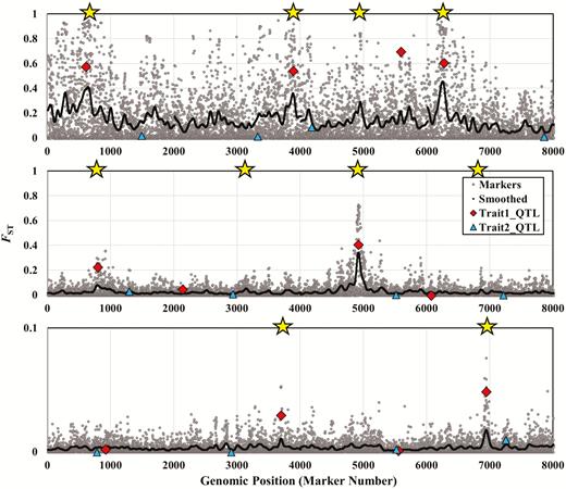
Manhattan plots for 3 typical simulation runs, under 3 different migration rates, in the absence of pleiotropy or epistasis. These simulations were run using the same parameter values as those used to generate the data in Table 2. Here, we use migration rates of m = 0.002 (top panel), m = 0.016 (middle panel), and m = 0.128 (bottom panel). The x axis shows genomic position, measured by the positions of marker loci. We simulated 2000 evenly spaced marker loci per linkage group and 4 linkage groups for a total of 8000 loci. Gray dots show the FST values for all marker loci, and the dark line shows smoothed FST values. We modeled one QTL for each trait per linkage group. FST values for QTL affecting trait 1 (with locally divergent optima) are shown as red diamonds, whereas FST values for QTL affecting trait 2 (with identical optima in both populations) are shown as blue triangles. Yellow stars at the top of each panel indicate smoothed FST peaks that were flagged as outliers by the 99% confidence interval method. All values shown here are from the final experimental generation of the simulation run (i.e., generation 2000).
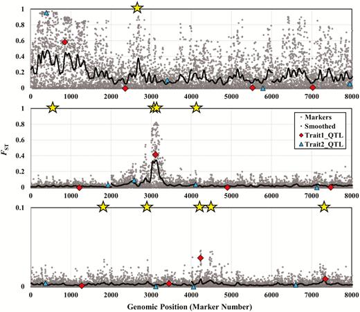
Manhattan plots for simulation runs including epistasis () under 3 different migration rates: m = 0.002 (top), m = 0.016 (middle), m = 0.128 (bottom). Simulation parameters for this figure are identical to those used for Figure 1, with the exception of epistatic parameters. See Figure 1 for an explanation of the symbols.
Another pattern apparent in Figure 1 is that the QTL for trait 1 tend to have elevated FST values, relative to markers, but in many cases only 1 or 2 QTL show these elevated values (Figure 1, middle and bottom). The QTL for trait 2, in contrast, almost universally exhibit FST values near 0 (Figure 1, blue triangles). Finally, if we examine the locations of the yellow stars, which represent smoothed outlier peaks, we see that many of the peaks do correspond to trait 1 QTL. However, spurious peaks also occur, and in some cases, they are as convincing as the peaks corresponding to QTL (Figure 1).
Figure 2 shows sample Manhattan plots in the presence of epistasis, and we see that these plots are qualitatively similar to those in Figure 1. The main difference, which emerges especially in our in-depth analysis below but is also apparent in the top panel of Figure 2, is that now QTL for trait 2 also sometimes show elevated FST values. Thus, in the presence of epistasis, QTL for trait 1 or trait 2 can be responsible for the trait 1 divergence that we observe between populations. The top panel of Figure 2 also shows how the detection of loci likely depends on the choice of smoothing parameters. The leftmost QTL, for instance, might be detectable with more smoothing, but at the cost of the regions of detection spanning much larger chromosomal segments. Similarly, in the middle panel of Figure 2, the single detected QTL (near genomic position 3100) produces 2 peaks, resulting in 2 apparent detections, but would be reduced to 1 peak with additional smoothing.
Figure 3 shows sample Manhattan plots for a genetic architecture in which all loci are pleiotropic, for a single migration rate (0.016) with and without epistasis. With pleiotropy, we see essentially the same patterns that we saw without pleiotropy, except now there is no distinction between QTL for trait 1 and trait 2.

Manhattan plots, similar to those shown in Figures 1 and 2, the top panel shows a genetic architecture including pleiotropy with no epistasis while the bottom panel shows pleiotropy with epistasis (where the epistatic parameter variance is equal to 1.6). Both panels show results from simulations with a migration rate of m = 0.016. Symbols and parameter values are described in Figure 1. Now, however, the QTL are shown as purple circles, with one QTL per linkage group. As the loci are pleiotropic, each QTL affects both traits.
Detection of Outlier Loci: Effects of Pleiotropy and Epistasis
Table 4 compares the results of outlier analyses under different migration rates in the absence and in the presence of epistasis (without pleiotropy). As migration rates increase, we see a substantial drop in mean marker FST values, as expected. As a result of selection on trait 1, the mean FST for trait 1 QTL is always larger than the mean marker FST. This effect occurs with or without epistasis (cf. top and bottom of Table 4). We see a different pattern for trait 2 QTL. In the absence of epistasis, the QTL for trait 2 have FST values that tend to be near (or even below) the values of the marker loci, consistent with the lack of divergent selection on these loci. In the presence of epistasis, however, the QTL affecting trait 2 also affect trait 1 through epistatic interactions, and we see these effects reflected in FST values that are larger than those of the mean marker values.
The results of outlier analyses for different migration rates without pleiotropy
| m | Mean marker FST | Mean Trt 1 QTL FST | Mean Trt 2 QTL FST | No. Smoothed FST Outliers | No. Near Trait 1 QTL | No. Near Trait 2 QTL | No. W&L FST Outliers | No. Near Trt 1 QTL | No. Near Trt 2 QTL | |
|---|---|---|---|---|---|---|---|---|---|---|
| 0 | 0 | 0.5842 | 0.7538 | 0.7520 | 1.067 | 0.033 | 0.033 | 0 | 0 | 0 |
| 0.002 | 0 | 0.1450 | 0.4862 | 0.1410 | 3.833 | 1.467 | 0.067 | 0 | 0 | 0 |
| 0.004 | 0 | 0.0874 | 0.3891 | 0.0655 | 4.633 | 1.667 | 0.067 | 1.967 | 0.500 | 0.033 |
| 0.008 | 0 | 0.0502 | 0.3038 | 0.0454 | 4.433 | 2.000 | 0.200 | 4.500 | 1.633 | 0.133 |
| 0.016 | 0 | 0.0292 | 0.2186 | 0.0232 | 4.467 | 1.900 | 0.067 | 5.800 | 2.000 | 0.100 |
| 0.032 | 0 | 0.0157 | 0.1476 | 0.0106 | 4.600 | 1.667 | 0.033 | 6.533 | 1.600 | 0.000 |
| 0.064 | 0 | 0.0076 | 0.0774 | 0.0089 | 4.333 | 1.700 | 0.033 | 7.200 | 1.767 | 0.200 |
| 0.128 | 0 | 0.0039 | 0.0299 | 0.0040 | 4.467 | 1.633 | 0.067 | 9.200 | 1.500 | 0.333 |
| 0.256 | 0 | 0.0025 | 0.0034 | 0.0025 | 4.767 | 0.233 | 0.100 | 9.533 | 0.333 | 0.300 |
| 0 | 1.6 | 0.5820 | 0.8308 | 0.8513 | 1.533 | 0.000 | 0.100 | 0 | 0 | 0 |
| 0.002 | 1.6 | 0.1605 | 0.3556 | 0.2788 | 2.933 | 0.433 | 0.333 | 0 | 0 | 0 |
| 0.004 | 1.6 | 0.0954 | 0.2915 | 0.1697 | 4.100 | 0.967 | 0.467 | 1.333 | 0.100 | 0.067 |
| 0.008 | 1.6 | 0.0569 | 0.1930 | 0.1373 | 4.333 | 1.033 | 0.633 | 3.667 | 0.567 | 0.467 |
| 0.016 | 1.6 | 0.0312 | 0.1466 | 0.0985 | 4.367 | 0.867 | 0.667 | 5.700 | 0.800 | 0.567 |
| 0.032 | 1.6 | 0.0158 | 0.1124 | 0.0508 | 4.367 | 1.000 | 0.433 | 6.667 | 1.067 | 0.500 |
| 0.064 | 1.6 | 0.0081 | 0.0616 | 0.0197 | 4.067 | 1.067 | 0.367 | 7.833 | 1.033 | 0.633 |
| 0.128 | 1.6 | 0.0037 | 0.0219 | 0.0079 | 4.533 | 0.800 | 0.300 | 8.867 | 0.967 | 0.433 |
| 0.256 | 1.6 | 0.0024 | 0.0033 | 0.0027 | 4.533 | 0.300 | 0.200 | 11.300 | 0.467 | 0.300 |
Parameter values are the same as in Table 2. Columns show the migration rate (m), the variance in epistatic parameters (), and mean FST values for marker loci (8000 loci total) and QTL affecting trait 1 and trait 2 (4 nonpleiotropic QTL for each trait). The next 3 columns show the number of outlier loci detected as smoothed FST peaks outside the 99% confidence interval of smoothed FST values, as well as the number of these peaks that fell within 25 marker loci of a trait 1 QTL or a trait 2 QTL. The final 3 columns show similar results using the Whitlock and Lotterhos (2015) method for detecting outliers with the degrees of freedom assumed to have a value of 1 and α = 0.01 (see Methods). Each entry in this table is a mean from 30 independent simulation runs under the relevant parameter combination.
In the absence of epistasis and pleiotropy (Table 4, top rows), we see that the number of QTL correctly detected by outlier analyses depends strongly on the migration rate. With migration rates of 0, all detections are spurious, because the populations do not even share alleles at their QTL. For migration rates above 0, the number of detected outlier peaks is remarkably consistent when we use smoothed FST values, ranging from 3.8 to 4.8. If we use the Whitlock and Lotterhos (2015) method, we see an increase in outlier peak detections (from 0 to 9.5) as the migration rate increases (but note that we did not use their iterative method to correct the degrees of freedom). Regardless of the number of apparent QTL detections with either method, the number of true detections (Table 4) reaches a maximum of about 2 QTL at a migration rate of 0.008 or 0.016. For lower or higher migration rates, the number of true QTL detections declines. Thus, never do we detect more than about half of the 4 QTL affecting trait 1 in this favorable scenario with a very simple genetic architecture.
When epistasis is included in the model (Table 4, bottom rows), our power to detect true outlier loci diminishes. In virtually all cases, we detect substantially fewer QTL for trait 1 than in the absence of epistasis. We do detect some QTL affecting trait 2 as actual outlier loci, but even taking these into account, we have fewer total detections of true QTL under epistasis than in the absence of epistasis.
Table 5 shows an analysis similar to that shown in Table 4, but with pleiotropy included in the genetic architecture. Interestingly, almost the same patterns emerge as we observed in the absence of pleiotropy. In particular, the total number of outlier peaks identified by each method is similar, and the true QTL detections reach a maximum of about 2, with more true positives occurring for intermediate migration rates. The addition of epistasis diminishes the number of true detections, but the total number of pleiotropic loci correctly detected in the presence of epistasis (Table 5) is nearly the same as the sum of trait 1 and trait 2 QTL detected for nonpleiotropic loci with epistasis (Table 4).
The results of outlier analyses when all loci are pleiotropic
| m | Mean marker FST | Mean pleiotropic QTL FST | No. smoothed FST outliers | No. near pleiotropic QTL | No. W&L FST outliers | No. near pleiotropic QTL | |
|---|---|---|---|---|---|---|---|
| 0 | 0 | 0.5839 | 0.7894 | 1.167 | 0.000 | 0 | 0 |
| 0.002 | 0 | 0.1463 | 0.4973 | 3.700 | 1.667 | 0 | 0 |
| 0.004 | 0 | 0.0907 | 0.4130 | 4.300 | 1.733 | 1.567 | 0.300 |
| 0.008 | 0 | 0.0532 | 0.3173 | 4.433 | 1.933 | 3.967 | 1.567 |
| 0.016 | 0 | 0.0290 | 0.2188 | 4.500 | 1.867 | 5.633 | 1.833 |
| 0.032 | 0 | 0.0152 | 0.1480 | 4.500 | 1.933 | 6.967 | 1.867 |
| 0.064 | 0 | 0.0074 | 0.0809 | 4.267 | 1.567 | 7.133 | 1.600 |
| 0.128 | 0 | 0.0038 | 0.0285 | 4.267 | 1.300 | 8.833 | 1.300 |
| 0.256 | 0 | 0.0025 | 0.0031 | 4.633 | 0.167 | 9.833 | 0.267 |
| 0 | 1.6 | 0.5841 | 0.9085 | 1.367 | 0.033 | 0 | 0 |
| 0.002 | 1.6 | 0.1593 | 0.4747 | 3.000 | 0.733 | 0.133 | 0.033 |
| 0.004 | 1.6 | 0.0972 | 0.3971 | 4.633 | 1.433 | 1.300 | 0.100 |
| 0.008 | 1.6 | 0.0575 | 0.2955 | 4.433 | 1.667 | 3.467 | 1.000 |
| 0.016 | 1.6 | 0.0314 | 0.2151 | 4.200 | 1.567 | 5.133 | 1.433 |
| 0.032 | 1.6 | 0.0159 | 0.1360 | 4.300 | 1.200 | 6.700 | 1.467 |
| 0.064 | 1.6 | 0.0085 | 0.0831 | 4.567 | 1.233 | 7.633 | 1.433 |
| 0.128 | 1.6 | 0.0037 | 0.0238 | 4.333 | 0.933 | 8.767 | 1.000 |
| 0.256 | 1.6 | 0.0023 | 0.0021 | 4.567 | 0.167 | 10.733 | 0.333 |
This table shows the migration rate (m), the variance in epistatic parameters (), mean FST values for markers and QTL, and results of 2 different methods for outlier detection. In contrast to the results shown in Table 4, we no longer distinguish between trait 1 and trait 2 loci, because pleiotropic loci affect both traits. The last 4 columns show the number of outlier marker loci detected by the 99% confidence interval approach and the Whitlock and Lotterhos (2015) approach. In each case, we also show the number of these outlier peaks that fell within 25 marker loci of a QTL on the relevant linkage group.
Understanding the QTL
Some additional explanation is necessary to make sense of the patterns we see regarding QTL detection by FST outlier analysis. These analyses also reveal that refinement of the method of outlier analysis probably would not help much for a 2-population comparison like the one we present here.
First, we consider the distribution of FST values for the QTL in our study. Figure 4 shows histograms of FST for trait 1 and trait 2 QTL for 30 replicates of the simulation under a migration rate of 0.016 (i.e., a favorable migration rate for outlier detection). Without epistasis (Figure 4, upper left), the distribution of trait 1 QTL FST values has a large peak near 0 and a substantial tail stretching out toward a value of 0.8. Nearly all of the QTL with FST values above about 0.2 were detected as outliers. Thus, some trait 1 QTL make no contribution to population divergence, have low FST values, and would not be detected by any FST outlier approach. Another set of QTL appears to contribute to population divergence, displays larger FST values, and is easily detected by the smoothed FST outlier approach we use in the present study. Even under the favorable conditions simulated for Figure 4, a third of the QTL for trait 1 have FST values near 0. In the absence of epistasis, all QTL for trait 2 have low FST values (Figure 4, upper right), and none are detected in outlier scans, except for 2 spurious detections.
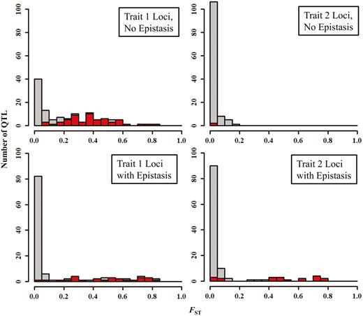
Histograms showing the distributions of trait 1 and trait 2 QTL FST values with and without epistasis in the absence of pleiotropy. These results are compiled from 30 simulation runs with 4 linkage groups and 1 QTL for each trait per linkage group (for a total of 120 QTL). The migration rate is 0.016, and other parameter combinations are identical to those used for Table 2. Bars are colored based on whether the QTL was detected as an outlier, with gray indicating QTL that were not detected and red indicating QTL that were detected. The histograms on the left show results for trait 1 and those on the right show results for trait 2. The top row shows results without epistasis and the bottom row shows results with epistasis (). In the absence of epistasis, trait 1 loci (upper left) with large FST values were almost always detected, as indicated by the abundance of red in the bars corresponding to FST larger than 0.2. Note that all detections are for marker loci in the vicinity of the QTL, as QTL FST values are assumed to be unknown to the researcher. The trait 2 loci (upper right) almost always had small FST values and almost none were implicated as outliers. The few that were identified as outliers reflect spurious coincidences (as do apparent detections of QTL with FST values near 0). The lower half of the figure shows a very different pattern in the presence of epistasis. The number of trait 1 loci with large FST values is substantially diminished (lower left), resulting in fewer outlier detections. In addition, now a number of trait 2 loci have large FST values (lower right) and are implicated as legitimate outliers. This result occurs because the trait 2 loci now affect trait 1 through their epistatic interactions with trait 1 loci.
In the presence of epistasis, the distinction between loci that do and do not contribute to population divergence is even clearer (Figure 4, lower panels). Again, the loci contributing to population divergence have values of FST larger than about 0.2 and are readily detected in outlier scans. Now, however, two thirds of trait 1 QTL have FST values near 0, rendering them undetectable by any method that uses an FST outlier approach. We also see that epistasis results in a distribution of FST values for trait 2 QTL that is more similar to the distribution for trait 1 QTL (Figure 4, bottom right), in comparison to the scenario without epistasis (Figure 4, upper vs. lower).
An important question concerns how much the QTL detected by outlier scans contribute to population divergence in trait values. This issue is addressed by Figure 5, which shows the relationship between the between-population difference in mean allelic effect and the FST for the QTL depicted in Figure 4. The between-population difference in mean allelic effect is calculated on a per-locus basis, as the mean genotypic value (both alleles summed within an individual) across individuals within population 1 minus the same quantity calculated for the same locus in population 2. Thus, loci with larger values make larger contributions to the difference in trait means across populations. For epistatic loci, we use the reference effect, so this between-population difference could be modified substantially by epistatic effects in the actual population. For trait 1 QTL, we see a positive relationship (linear regression, P << 0.0001, R2 = 0.81), indicating that loci with the most divergent allelic effects also have the most divergent allele frequencies (Figure 5, left panels). This effect occurs regardless of the presence of epistasis (cf. Figure 5, upper left to Figure 5, lower left; with epistasis: linear regression of FST on absolute mean allelic effect difference, P <<< 0.0001, R2 = 0.48). Interestingly, with epistasis, we see one outlier with an allelic difference in opposition to the trait mean difference between populations. This phenomenon stems from negative epistasis, which can change negative reference effects into positive contributions to the trait value.
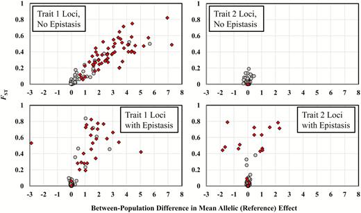
The relationship between the between-population difference in mean allelic effects and FST for trait 1 and trait 2 QTL in the absence and presence of epistasis. The between population difference in allelic effect is calculated on a per-locus basis as the average allelic effect in population 1 minus the average allelic effect in population 2. In the absence of epistasis, these effects are additive effects, and in the presence of epistasis we use reference effects for simplicity. These values are typically positive for trait 1 loci because population 1 has a trait 1 optimum of 4 and population 2 has a trait 1 optimum of −4. Each point represents a single QTL, with red diamonds indicating loci that were identified as outliers and gray circles representing loci that were not flagged as outliers. With or without epistasis, loci with larger differences in additive (or reference effects) tend to have larger FST values and tend to be detected as outliers. In the absence of epistasis, trait 2 loci (upper right panel) tend to differ very little among populations and show low FST values, as expected given that the populations have identical trait 2 optima. However, in the presence of epistasis (lower right panel), we now see more divergence among populations in trait 2 locus reference effects and more trait 2 loci with high FST values. The sign of divergence in trait 2 reference effects depends on the values of epistatic parameters corresponding to these loci. Parameter values for this figure are the same as those used for Table 2, with a migration rate of 0.016.
Two other important patterns are shown in Figure 5. First, almost all of the loci with large effects on the between-population divergence in trait values were detected as outliers in our analysis (Figure 5, left panels, red diamonds). Second, the pattern for trait 2 QTL differs substantially from that for trait 1 QTL. In particular, in the absence of epistasis, trait 2 QTL show almost no meaningful divergence. However, in the presence of epistasis, trait 2 QTL do show divergence, but without the predictable directionality we see in trait 1 QTL. This latter result occurs because trait 2 QTL affect trait 1 only indirectly through epistatic interactions with trait 1 loci, whereas trait 1 QTL affect trait 1 directly via reference effects and indirectly through interactions with each other and with trait 2 loci.
Figure 6 shows analyses that correspond to those shown in Figures 4 and 5 but for pleiotropic loci. The distribution of FST values for pleiotropic QTL is very similar to that for trait 1 QTL in the absence of pleiotropy (Figure 6, top panel; Figure 4, upper left). In addition, the relationship between population divergence in allelic effects and FST for pleiotropic loci also mirrors that for trait 1 QTL (Figure 6, middle panel compared with Figure 5, upper left; with pleiotropy: linear regression, P <<< 0.0001, R2 = 0.88). However, the relationship between the trait 2 between-population difference in allelic effects and FST is quite different, as pleiotropic QTL display a wider range of between-population differences in allelic effects (relative to nonpleiotropic trait 2 QTL). These differences occur whenever a pleiotropic locus with a favorable effect on trait 1 carries a relatively large pleiotropic effect on trait 2 along with it as it diverges. However, we see no clear relationship between divergence in allelic effects at trait 2 and the value of FST for pleiotropic loci (Figure 6, bottom panel).
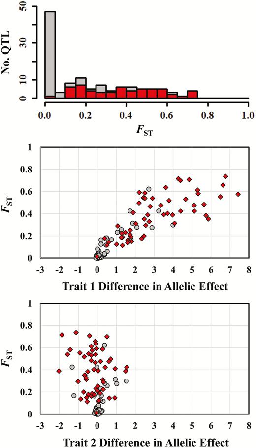
Patterns of FST for pleiotropic QTL in the absence of epistasis. Shown are the histogram of QTL FST values for pleiotropic loci (top), FST as a function of the per-locus between-population differences in allelic effects for trait 1 (middle panel), and FST as a function of the per-locus between-population differences in allelic effects for trait 2 (bottom panel). As in Figure 4, the histogram (top) shows detected loci in red and undetected loci in gray. In the middle and bottom panels, loci flagged as outliers are shown as red diamonds and undetected loci are shown as gray circles. The results from this figure are from 30 simulations run under the parameter combinations used to produce Table 3, with a migration rate of 0.016.
The relationship between divergence in allelic effects and the contribution to within-population genetic variance on a locus-per-locus basis is addressed in Figure 7. Regardless of the genetic architecture, loci with the largest divergence among populations in allelic effects make the largest contributions to within-population genetic variance (Figure 7; linear regressions: no epistasis or pleiotropy: P <<< 0.0001, R2 = 0.92, only pleiotropy: P <<< 0.0001, R2 = 0.91, only epistasis: P <<< 0.0001, R2 = 0.77). This result makes sense because alleles contributing to the difference in trait means between populations will tend to have allelic effects that are typical for their population of origin but quite different from the alleles segregating in the other population. While selection will oppose the migration of these alleles, those that do successfully migrate will substantially increase the genetic variance for the trait in the recipient population. This result also means that the loci making the largest contributions to within-population variance in trait values are the most detectable in genome-wide scans (because they also contribute to population divergence).
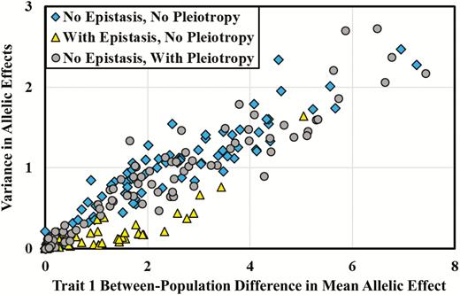
The relationship between the between-population difference in mean allelic effects and the within-population variance in allelic effects with and without epistasis and pleiotropy. The results shown in this figure are from 30 simulation runs under parameter values identical to those used in Figures 4–6. Results are shown for simulations without epistasis and without pleiotropy (blue diamonds), with epistasis but without pleiotropy (yellow triangles), and without epistasis but with pleiotropy (gray circles). Values on the x axis are calculated as the absolute value of the mean trait 1 allelic effect in population 1 minus the mean trait 1 allelic effect in population 2, because we care here about the absolute difference among populations regardless of the sign. Values on the y axis are calculated as the variance among individuals in genotypic values at the locus in question, where the genotypic values are calculated as the sum of the 2 allelic effects (or reference effects) at the relevant locus in a given individual. This figure indicates a universal tendency for the loci with the largest differences in allelic effects between populations to make the largest contribution to the additive genetic variance within populations.
In summary, we can draw the following generalizations, regardless of whether the genetic architecture includes epistasis or not: QTL with the largest between-population differences in allelic effects also have the highest FST values and are the most detectable in genome-wide scans for FST outliers. These loci also make the largest contribution to within-population genetic variance. Thus, genome-wide scans for FST outliers associated with local adaptation likely detect some, but not all, important QTL, and those that are detected will tend to be the loci that make the largest contributions to divergence and within-population genetic variance.
Sensitivity to Assumptions
The results described above seem to be relatively insensitive to assumptions regarding parameter values. Obviously, the migration rate is important, as are the distance between optima and the strength of selection. An exploration of other parameter values, however, reveals some surprising trends, which we discuss here. A subset of relevant simulation results is shown in Table 6.
The effects of various parameters on FST outlier analyses
| Variable of interest and its value | Mean marker FST | Mean Trt 1 QTL FST | Mean Trt 2 QTL FST | No. smoothed FST outliers | No. near Trt 1 QTL | No. near Trt 2 QTL | No. W&L FST outliers | No. near Trt 1 QTL | No. near Trt 2 QTL | |
|---|---|---|---|---|---|---|---|---|---|---|
| Carrying capacity | ||||||||||
| K = 250 | 0 | 0.0172 | 0.1046 | 0.0175 | 4.800 | 1.700 | 0.133 | 3.533 | 1.433 | 0.067 |
| K = 250 | 1.6 | 0.0172 | 0.0461 | 0.0484 | 5.300 | 0.700 | 0.867 | 3.500 | 0.633 | 0.733 |
| K = 4000 | 0 | 0.0380 | 0.1415 | 0.0382 | 4.333 | 2.433 | 0.200 | 5.000 | 2.333 | 0.200 |
| K = 4000 | 1.6 | 0.0409 | 0.1499 | 0.0741 | 3.967 | 1.700 | 0.467 | 4.867 | 1.533 | 0.667 |
| Sample size | ||||||||||
| S = 10 | 0 | 0.0433 | 0.1641 | 0.0445 | 4.767 | 1.733 | 0.300 | 3.500 | 1.200 | 0.100 |
| S = 10 | 1.6 | 0.0453 | 0.0868 | 0.0810 | 4.500 | 0.800 | 0.733 | 3.667 | 0.500 | 0.467 |
| S = 500 | 0 | 0.0271 | 0.1271 | 0.0284 | 4.700 | 1.967 | 0.333 | 6.333 | 2.067 | 0.567 |
| S = 500 | 1.6 | 0.0300 | 0.0765 | 0.0795 | 4.767 | 0.900 | 0.667 | 6.000 | 0.933 | 0.833 |
| Selection strength | ||||||||||
| ω11 = 19 | 0 | 0.0922 | 0.3091 | 0.0757 | 4.500 | 1.633 | 0.267 | 2.133 | 0.600 | 0.167 |
| ω11 = 19 | 1.6 | 0.1081 | 0.2356 | 0.1925 | 4.267 | 1.000 | 0.633 | 1.767 | 0.067 | 0.067 |
| ω11 = 99 | 0 | 0.0177 | 0.0761 | 0.0163 | 4.633 | 1.567 | 0.133 | 6.967 | 1.733 | 0.400 |
| ω11 = 99 | 1.6 | 0.0182 | 0.0550 | 0.0382 | 4.467 | 0.867 | 0.600 | 6.067 | 0.867 | 0.667 |
| Epistasis amount | ||||||||||
| = 0.4 | 0.4 | 0.0306 | 0.1075 | 0.0480 | 4.667 | 1.200 | 0.433 | 5.467 | 1.200 | 0.567 |
| = 0.8 | 0.8 | 0.0296 | 0.1005 | 0.0605 | 4.900 | 1.167 | 0.567 | 6.000 | 1.233 | 0.600 |
| = 3.2 | 3.2 | 0.0313 | 0.0752 | 0.686 | 4.433 | 0.900 | 0.633 | 5.867 | 0.900 | 0.600 |
| = 6.4 | 6.4 | 0.308 | 0.0879 | 0.0710 | 4.433 | 0.933 | 0.633 | 5.933 | 0.933 | 0.633 |
| No. marker loci per linkage group | ||||||||||
| nm = 500 | 0 | 0.0305 | 0.1459 | 0.0270 | 1.700 | 1.100 | 0.467 | 2.333 | 1.533 | 0.533 |
| nm = 500 | 1.6 | 0.0306 | 0.1035 | 0.0633 | 1.533 | 0.833 | 0.533 | 2.467 | 1.233 | 0.867 |
| nm = 10 000 | 0 | 0.0285 | 0.1399 | 0.0326 | 14.800 | 1.833 | 0.167 | 17.067 | 1.633 | 0.133 |
| nm = 10 000 | 1.6 | 0.0313 | 0.1021 | 0.0575 | 16.333 | 0.767 | 0.433 | 15.400 | 0.800 | 0.333 |
| No. QTL per linkage group | ||||||||||
| nq1 = nq2 = 2 | 0 | 0.0289 | 0.1372 | 0.0291 | 4.900 | 2.033 | 0.267 | 5.967 | 2.100 | 0.333 |
| nq1 = nq2 = 2 | 1.6 | 0.0301 | 0.0984 | 0.0601 | 4.933 | 0.933 | 0.667 | 5.733 | 0.900 | 0.833 |
| nq1 = nq2 = 5 | 0 | 0.0273 | 0.0730 | 0.0284 | 4.467 | 2.333 | 0.533 | 5.267 | 2.333 | 0.700 |
| nq1 = nq2 = 5 | 1.6 | 0.0287 | 0.0544 | 0.0407 | 4.900 | 1.467 | 0.900 | 5.267 | 1.367 | 1.100 |
| Recomb. rate | ||||||||||
| R = 0.10 | 0 | 0.0394 | 0.1442 | 0.0350 | 4.300 | 1.500 | 0.167 | 2.933 | 0.900 | 0.033 |
| R = 0.10 | 1.6 | 0.0401 | 0.1104 | 0.0687 | 4.267 | 0.867 | 0.633 | 3.200 | 0.467 | 0.333 |
| R = 4.00 | 0 | 0.0209 | 0.1166 | 0.0180 | 4.133 | 1.567 | 0.100 | 9.567 | 1.700 | 0.633 |
| R = 4.00 | 1.6 | 0.0222 | 0.0827 | 0.0466 | 3.567 | 0.967 | 0.633 | 9.300 | 1.200 | 0.767 |
Results shown here assume no pleiotropy, but the qualitative patterns are similar whether or not loci are pleiotropic. We also assume 2 QTL per linkage group per trait, resulting in a total of 8 QTL per trait, except where noted. Except for the parameter being perturbed (indicated in the first column), the epistatic parameter variance (indicated in the second column), and the number of QTL per trait, all other parameter values are identical to those listed in Table 1. In the case of carrying capacity, the migration rate is adjusted to keep the number of migrants, rather than the migration rate, constant as the population size varies. Column labels for columns 3 through 11 have the same meaning as in Table 4.
The results shown in Table 6 differ from most of our other results in that we now simulate 2 QTL per linkage group (with 4 linkage groups) meaning that each trait is determined by 8 QTL. Despite this change, the number of outlier peaks (identified by the smoothed FST approach) remains near 4 or 5 for almost all parameter combinations, with a maximum mean of 2.4 true QTL detections (Table 6).
For most of our simulations, we use a carrying capacity of 500 (resulting in an adult population size of 500). We find that the number of outlier peaks does not change much with increasing population size, but that larger populations are more likely to produce true QTL detections (Table 6). The detection of peaks is somewhat affected by sample size, but detections are still possible with a sample of as few as 10 individuals per population (Table 6). Intermediate strengths of selection are most favorable for the detection of outlier loci, as very weak selection produces no population divergence (i.e., the effects of migration swamp out the effects of selection) and very strong selection limits migration, as migrants die before they can contribute to the gene pool (Table 6).
We also find that the amount of epistasis affects the detection of QTL. As the epistatic variance gets larger (Table 6), the number of trait 1 QTL detected decreases slightly and the number of trait 2 QTL detected increases slightly. This pattern should be expected, as stronger epistasis increases the potential for trait 2 QTL to drive population divergence in trait 1 means.
The number of marker loci per linkage group greatly affects the number of identified outlier peaks (Table 6). A very small number of loci (500 per linkage group), results in fewer peaks and fewer detections. A large number of loci (10 000 per linkage group), greatly increases the number of false positives without substantially increasing the number of true QTL detections.
Oddly enough, increasing the number of QTL per linkage group has almost no effect on the number of true QTL detections (Table 6). Even with 5 QTL per linkage group, resulting in 20 QTL for each trait, only about 2 true QTL are detected, regardless of the outlier method. Inspection of individual runs and distributions of QTL effects show that regardless of the underlying number of QTL, only a small number ever contribute substantially to population divergence. Thus, the failure to detect QTL is a consequence of the biological system more than the techniques used to detect them.
Finally, the simulations are surprisingly insensitive to recombination rate (Table 6). Even with a 40-fold change in recombination rate per linkage group (from 0.10 to 4), the number of QTL detected remains relatively stable, although we do see a difference between the smoothed outlier approach and the Whitlock and Lotterhos (2015) approach here.
Discussion
In this report, we use a simulation-based approach to model a genetic architecture including pleiotropy and epistasis, which allows us to test the hypothesis that these genetic complexities will impact the efficacy of genome-wide scans to detect outlier loci responsible for local adaptation. Our model differs from most other such models in that we explicitly simulate the underlying quantitative-genetic architecture, including a specified number of quantitative trait loci, and use these loci to determine individual trait values. Selection then acts on the trait values, rather than directly on the underlying loci. We also model a suite of marker loci, explicitly located on linkage groups, and place our QTL randomly on these linkage groups. After a period of evolution and divergence among populations, we simulate a genome-wide study of SNPs and ask whether the study can identify outlier loci associated with the QTL.
Regardless of the number of QTL, the mean number of true QTL detections is never much larger than 2, and we generally find at least as many false positives as true positives. Encouragingly, loci making large contributions to population divergence and large contributions to within-population genetic variance are usually detectable. However, in the type of system we model here, most population divergence is caused by a small number of loci (often 1 or 2), even when the genetic architecture is highly polygenic. Our results also show that pleiotropy has almost no effect on the success of genome-wide scans for outlier loci. Epistasis, on the other hand, reduces the efficacy of genome-wide scans for QTL by spreading the signal of selection across a larger number of interacting loci, relative to a strictly additive genetic architecture.
The Evolution of the Genetic Architecture
Regardless of the genetic architecture under consideration, the simulated populations evolve toward their optima, with the position of the population mean determined by a migration-selection balance (King and Lawson 1995; Hendry et al. 2001). As expected, low migration rates result in population means near their respective optima. As the migration rate increases, each population is displaced further from its optimum, and we see a dramatic increase in the additive genetic variance, as maladaptive alleles migrate into each population. This phenomenon is identical to the situation modeled by Guillaume and Whitlock (2007), who observed that migration tends to stretch the G-matrix in the direction of the optimum of the population from which the migrants originated. Interestingly, in our model most of the divergence and the increase in genetic variance are caused by a small number of QTL, as the majority of QTL have FST values near 0 and make small contributions to the additive genetic variance. When the migration rate becomes extremely high, the populations essentially behave as a single panmictic group, with a mean near the midpoint between the population optima. In this case, we see an increase in additive genetic variance relative to the case with no migration as a consequence of spatially varying selection.
In the absence of pleiotropy, the 2 traits evolve nearly independently. When the 2 populations have different trait 1 optima but identical trait 2 optima, trait 2 remains near its optimum, regardless of the change in the mean of trait 1. We see a very slight increase in additive genetic variance in trait 2 as the additive genetic variance for trait 1 increases, probably caused by occasional trait 2 loci that are tightly linked to nearby trait 1 loci.
With the addition of pleiotropy to the model, the most dramatic effect is that any increase in additive genetic variance in trait 1 also results in an increase in additive genetic variance in trait 2. This effect is a well understood consequence of pleiotropy (Lande 1980; Turelli 1985; Bürger and Krall 2004). The fact that each locus affects both traits results in a situation in which any mechanism impacting the genetic variance of one trait also alters the genetic variance, often to a lesser degree, of any pleiotropically linked trait. Our simulations also reveal a trend for trait 1 to exhibit less additive genetic variance under pleiotropy than in the absence of pleiotropy (Lande 1980; Turelli 1985; Bürger and Krall 2004), and this reduction is caused by the loss of some alleles contributing to variation in trait 1 as a consequence of stabilizing selection on trait 2.
Our study is among the first to examine population divergence under the multilinear model of epistasis (Hansen and Wagner 2001; Fierst and Hansen 2010; Jones et al. 2014). Regardless of the magnitude of the variance in epistatic parameters (i.e., the absolute magnitude of epistasis), most of the genetic variance for the quantitative traits in our model ends up being additive genetic variance, a result typical for the multilinear model (Carter et al. 2005; Jones et al. 2014). In addition, population differentiation seems to result in an even higher proportion of the genetic variance being additive than would occur for populations with identical optima (or a single population evolving in isolation). For instance, in 2 populations with identical trait 1 optima of 0, assuming an epistatic parameter variance of 6.4 and 12 pleiotropic QTL, the total genetic variance for trait 1 is 0.206, and the corresponding additive genetic variance is 0.181, so 88% of the genetic variance for trait 1 is additive. Under the same circumstances, except with trait 1 optima of 4 and −4 for the 2 populations, the total genetic variance for trait 1 is 3.376 and the additive genetic variance is 3.263, so now 97% of the total genetic variance is additive. This increase in additive genetic variance is a consequence of much of the segregating variation within each population arising from loci with large between-population differences in reference effects. Individual loci with huge effects contribute mainly additive genetic variance to the population, especially when the populations are nearly identical with respect to most other QTL, as we observed in our model. Because nearly all of the genetic variance is additive in the scenarios we consider, we ignore the distinction everywhere in the present article, except in this section.
Given that our diverging populations possess mostly additive genetic variance, the observation that epistasis has only minor effects on population divergence (relative to the same architecture without epistasis) is not surprising. Rather, the extent of divergence seems to be driven mainly by the strength of selection and the rate of migration, as noted above. Thus, genetic effects of local adaptation require some gene flow but not too much, and the exact meaning of “some but not too much” depends on the selective regime and the demographics of the individual system. However, it does not seem to depend on the details of epistasis and pleiotropy, which should be a comforting result for most empiricists.
A few other studies of the evolution of the genetic architecture under the multilinear model provide some context for the present study. The most similar study to ours was conducted by Fierst and Hansen (2010), who investigated the evolution of Bateson–Dobzhansky–Muller (BDM) incompatibilities between 2 isolated populations. They modeled only one trait, allowed no migration, and assumed the same trait optimum in both populations. Nevertheless, they did observe genetic divergence at individual loci, as divergent alleles arose by mutation and rose to fixation in their population of origin. These evolving genetic architectures often gave rise to hybrid incompatibilities between the 2 populations. While an analysis of BDM incompatibilities was beyond the scope of the present article, future studies could profitably explore the evolution of such incompatibilities in a multiple-trait system involving populations with different optima linked by gene flow, as we studied here. Hermisson et al. (2003) studied a single population experiencing stabilizing selection, and showed that epistasis results in a reduction of additive genetic variance at mutation-selection balance. They also found that loci with high mutation rates tended to evolve smaller mutational effects compared with loci with low mutation rates (Hermisson et al. 2003). This line of inquiry was extended to populations experiencing fluctuating selection by Le Rouzic et al. (2013), who showed that unstable optima tended to counteract the evolution of canalization. These results (Hermisson et al. 2003; Le Rouzic et al. 2013) illustrate that epistasis plays a role in the evolution of evolvability and canalization (Hansen 2006), topics that would be interesting to study in an array of populations linked by gene flow.
Detecting Outlier Loci without Epistasis or Pleiotropy
When 2 populations diverge, with quantitative traits modeled according to a standard additive model like the one we used here, most of the divergence seems to involve huge differences in allelic effects at a small number of loci. Under most circumstances under consideration here, at least some outlier loci are detectable in our simulations. However, in no cases are all of the QTL identifiable as outliers, and the main cause of this constraint appears to be biological in the sense that loci making small contributions to population divergence tend to have low FST values. Ours is not the first study to conclude that most trait divergence involves a small number of QTL, as an analysis by Yeaman and Whitlock (2011) shows the same pattern, a result confirmed analytically by Geroldinger and Bürger (2014) in a 2-locus model. This tendency for a small number of QTL to diverge occurs despite the fact that all loci in our simulations were identical with respect to mutation rates and mutational variances. It also occurs regardless of the total number of QTL. For any number of modeled loci, including as many as 20 QTL per trait in some cases, our analyses never identified more than about 2.5 true QTL on average in the best-case scenarios. This finding is consistent with the work of Vilas et al. (2012), whose model uses a trait with a strictly additive genetic architecture without pleiotropy and applies selection at the level of the trait phenotype. Their results also indicate that most divergence involves a small number of QTL, resulting in most QTL being undetectable in genome-wide scans.
For outlier detection, we use simple approaches that are readily hard-coded into our simulation model. This approach allows a wider exploration of sample space, at the expense of ignoring methods that might perform better for outlier detection. Our goal here, however, is to examine how pleiotropy and epistasis affect outlier scans, rather than to systematically compare methods. In addition, our results show that the smoothed FST confidence interval approach detects nearly all of the QTL with appreciable FST values (Figures 4–6). The nondetected QTL have FST values that bury them in the broader sea of marker FSTs, rendering them undetectable without incurring an unacceptably high rate of Type II error.
Because we used simplified methods of outlier detection, our study should not be considered a test of the performance of the OUTFLANK package, which implements the Whitlock and Lotterhos (2015) approach. Several details of our approach differ from that implemented in OUTFLANK. First, we use all marker loci without pruning the dataset to include only loci with low linkage disequilibrium. Second, we use a χ2 distribution with 1 df (i.e., 1 − number of populations), while Whitlock and Lotterhos (2015) use an iterative process to remove outlying loci from the distribution before determining the appropriate χ2 distribution. Third, we test loci for significance only for markers near a smoothed FST peak, thus limiting tests to a smaller part of the genome. However, inspection of many plots like those shown in Figures 1–3 shows that our implementation almost always identifies large peaks as significant. By more carefully following the Whitlock and Lotterhos (2015) algorithm, we might have been able to reduce the number of false positives, but additional true positives would still have remained undetectable because undetected true positives tend to fall in genomic regions with unsubstantial FST peaks. Our analysis seems to indicate that the Whitlock and Lotterhos (2015) technique experiences an increase in false positives when the mean FST decreases or the number of marker loci increases, but these patterns should be disregarded until they are explicitly addressed in studies designed to test the performance of OUTFLANK per se.
Our demographic scenario also precludes many methods of analysis. For instance, the methods used by Fdist2 (Beaumont and Nichols 1996) and LOSITAN (Antao et al. 2008), based on the heterozygosity–FST relationship, perform poorly when only 2 populations are sampled (Flanagan and Jones 2017). Similarly, Bayenv (Günther and Coop 2013) and FLK (Bonhomme et al. 2010), two other recently developed methods, also perform better when more than 2 populations are sampled, as they correct for population history, a correction that has little meaning in the 2-population case. Other promising methods include those that use genetic–environment association approaches, such as those implemented by LFMM (Frichot et al. 2013) and PCAdapt (Duforet-Frebourg et al. 2014). Our simulations do not include environmental variables, however, so these methods also are not appropriate. All of these methods could profitably be explored in future studies using our approach to the genetic architecture but including a larger number of populations inhabiting a range of simulated habitat types.
Our results are probably somewhat dependent on assumptions regarding marker loci. We chose to allow a maximum of 4 alleles per locus, so the markers can be interpreted as SNPs. Our simulated markers behaved very much like actual SNPs, in the sense that they tended to have a common allele at a high frequency, with the other alleles being rare. For instance, in a sample run under the core parameter values, we found that the common allele had a mean frequency of 0.84 across all loci by the end of the simulation when outlier scans were conducted. This value for the major allele frequency would not be unexpected for real data, particularly if the researchers chose to use the more informative loci for their analysis. Under the core parameter values (Table 1), we also model a relatively small genome, in the sense that we model 4 chromosomes with a recombination rate of 0.25 per generation per chromosome. Thus, the total genome modeled here is only 100 centimorgans in length, and the linkage groups are probably best interpreted as parts of a genome. Larger genomes would almost certainly result in an increase in false positives and greater difficulties in detecting outlier loci. Our marker loci should also be interpreted as being in quite close proximity to one another. For instance, in a sample run under default parameter values (Table 1), the mean D′ between neighboring markers was 0.886. In addition, the location of a QTL is defined by its associated marker locus, so a QTL will usually be in strong linkage disequilibrium with at least 1 marker. Exceptions can occur when the marker locus loses all polymorphism or mutations reduce the linkage disequilibrium between a QTL and its location-defining marker. Regardless, our results (Figures 1–3) show that linkage disequilibrium does decay substantially across our linkage groups, and our Manhattan plots are not dissimilar from those observed in empirical studies of local adaptation.
Effects of Pleiotropy and Epistasis on Outlier Analysis
Adding pleiotropy to the genetic architecture of traits results in almost no change in the prospects for identifying QTL affecting the trait involved in local adaptation. The mean FST values for the QTL affecting trait 1 are approximately the same with and without pleiotropy, as are the number of apparent QTL detections and the proportion of these detections near true QTL (cf. Tables 4 and 5). Under pleiotropy, some of these loci have reasonably large differences between populations in their mean effects on trait 2, but apparently these differences play a minor role in aiding or preventing differentiation (see Figure 6, bottom panel). Here, we restrict attention to a bivariate optimum that moves only along the trait 1 axis. Presumably, movement in a different direction in bivariate phenotypic space would result in a stronger signal of selection on pleiotropic as compared to nonpleiotropic QTL.
The effects of epistasis on genome-wide scans for adaptive QTL are more pronounced, and they occur whether or not pleiotropy is also included in the model. In particular, epistasis universally decreases FST values for QTL affecting the trait involved in local adaptation, compared with the case without epistasis (Tables 4 and 5). This reduction in FST makes the causal QTL less detectable in genome-wide scans for outliers. While the number of apparent detections remains almost the same with and without epistasis, the proportion of these detections that represent true positives decreases. This result makes intuitive sense, because epistasis should spread the signature of selection across a greater number of loci, resulting in a weaker per-locus signal spread more evenly across the genome. A weak, diffuse signal will be less detectable than a strong, concentrated signal in a genome-wide scan. Interestingly, in the case of epistasis for nonpleiotropic loci, a substantial fraction of detected QTL have direct effects on trait 2. These loci affect trait 1 indirectly through their interactions with trait 1 QTL. Thus, in the presence of epistasis, detected loci include those with direct and indirect effects on the trait in question. Even factoring in the detected trait 2 QTL, however, genome-wide scans still detect fewer total QTL when epistasis is present than when it is absent. Nevertheless, some loci were detected, even with strong epistasis, indicating that an epistatic genetic architecture does not preclude success in the search for loci involved in local adaptation.
Caveats and Limitations of the Study
This study leaves a number of unanswered questions, and many other avenues are ripe for continued investigation. The biggest shortcoming of our article is that we model a very simple demographic scenario with only 2 populations linked by migration. More complex scenarios, with additional demes, will almost certainly result in different results in terms of how many QTL can be detected and which techniques are most appropriate. However, our scenario does have the advantage that pairwise population comparisons are possible in almost all population genetic studies. Nevertheless, future studies of the effects of epistasis and pleiotropy should endeavor to represent more complex demographic scenarios with more extensive sampling regimes.
Our study also uses only one model of gene interactions, the multilinear model. In this model, all loci have direct additive effects on one or both traits, as well as epistatic effects. Real gene networks may be quite different than those represented by the multilinear model. Thus, future work should investigate how the specific model of epistasis impacts migration-selection balance and the detection of outlier loci. We also use epistatic parameters drawn from a normal distribution with a mean of 0, resulting in no net positive or negative epistasis. Directional epistasis can have large impacts on evolutionary processes (Carter et al. 2005; Hansen 2013), so this phenomenon, too, is worthy of future study as it relates to local adaptation and population genomics. Some other genetic complications also could play a role in local adaptation and the detection of outlier loci. For example, our approach to modeling linkage groups did not allow for major chromosomal mutations, such as inversions, even though analytical theory indicates that structural rearrangements can facilitate local adaptation (Kirkpatrick and Barton 2006). In general, more realistic models of marker loci, gene networks, and chromosomal evolution in the context of population genomics approaches would be welcome additions to the literature.
As discussed above, our study also uses highly simplified methods for the detection of outlier loci. Our results show that these methods perform well in identifying FST peaks in our pairwise population comparisons and allow us to investigate the effects of the genetic architecture on the detection of outlier loci. However, future studies, modeling more realistic demographic scenarios, would certainly benefit from using more sophisticated techniques for outlier detection, most of which are not appropriate for the pairwise comparisons modeled here. In addition, recent simulation-based studies show that methods examining genetic–environment associations have greater power to detect loci involved in local adaptation (Lotterhos and Whitlock 2015). We did not model environmental variables, so a more comprehensive study involving environmental clines or possibly even multiple environmental variables selecting on multiple traits could reveal additional insights. In short, we need additional studies comparing outlier detection methods, a topic beyond the scope of the present study, and this need will grow as more analytical methods are developed in the near future.
Data Accessibility
All data reported in this work can be reproduced by using the associated simulation software, whose executables and source code are available from GitHub (https://github.com/JonesLabIdaho).
Acknowledgments
We are grateful to Anne Bronikowski for inviting our contribution to this special issue of Journal of Heredity devoted to the AGA Presidential Symposium entitled “Quantitative Genetics in the Wild.” We also would like to thank 2 anonymous referees, who provided valuable suggestions that improved this article.
