


Abstract
Multivariate quantitative genetics provides a powerful framework for understanding patterns and processes of phenotypic evolution. Quantitative genetics parameters, like trait heritability or the G-matrix for sets of traits, can be used to predict evolutionary response or to understand the evolutionary history of a population. These population-level approaches have proven to be extremely successful, but the underlying genetics of multivariate variation and evolutionary change typically remain a black box. Establishing a deeper empirical understanding of how individual genetic effects lead to genetic (co)variation is then crucial to our understanding of the evolutionary process. To delve into this black box, we exploit an experimental population of mice composed from lineages derived by artificial selection. We develop an approach to estimate the multivariate effect of loci and characterize these vectors of effects in terms of their magnitude and alignment with the direction of evolutionary divergence. Using these estimates, we reconstruct the traits in the ancestral populations and quantify how much of the divergence is due to genetic effects. Finally, we also use these vectors to decompose patterns of genetic covariation and examine the relationship between these components and the corresponding distribution of pleiotropic effects. We find that additive effects are much larger than dominance effects and are more closely aligned with the direction of selection and divergence, with larger effects being more aligned than smaller effects. Pleiotropic effects are highly variable but are, on average, modular. These results are consistent with pleiotropy being partly shaped by selection while reflecting underlying developmental constraints.
Individuals are composed of a complex array of traits that are interconnected through shared genetic, physiological, and developmental processes. Consequently, evolution is inherently a multivariate process, wherein suites of traits interact to determine an individual’s fitness, which generates selection that cascades to the genomic level through the genotype–phenotype relationship leading to heritable changes across generations (Lande and Arnold 1983; Klingenberg 2008; Melo et al. 2016). Therefore, understanding evolutionary change in response to selection requires an understanding of the relationship between genotypic variation and multivariate traits. The quantitative genetics framework was developed to achieve this goal, historically relying on statistical measurement of genetic covariation between traits as a summary of their genetic “connectedness.” The covariances estimated using this framework can be used to understand how sets of traits evolve together, including forward-looking predictions for the multivariate response to selection (Lande 1979) and the retrospective analysis of divergence by selective and neutral processes (Felsenstein 1988). The classical perspective in quantitative genetics, focused on statistical properties of trait covariation, can provide insights into these problems. However, it is limited by the fact that it treats the link between genotype and multivariate phenotype, which underlies patterns of covariation, as a black box. As a result, these approaches do not provide direct insights into the genetic architecture underlying patterns of genetic covariation, which ultimately determines how sets of interconnected traits evolve across generations. Therefore, an explicit link between the properties of the individual loci that underlie the multivariate genotype–phenotype relationship, and the associated consequences for patterns of genetic covariation are central to the study of evolution.
To understand the patterns of genetic covariation between traits, studies have taken a population level approach (top-down) that relies on pedigree relations to dissect components of phenotypic covariation. These studies are generally focused on understanding how variation constrains evolution or how covariation (in the statistical sense) itself evolves in relation to multivariate selection (Arnold et al. 2008; Futuyma 2010). The effect of covariation in constraining short-term evolution is well established: if traits covary genetically the evolution of a focal trait depends on the selection upon the traits it is correlated to. As a result, a trait that is not under selection can evolve as a correlated response to selection on other traits (Lande 1979; Grant and Grant 1995), and for traits under selection, their response can be reduced or enhanced due to antagonistic (where the correlated response opposes the direction of direct selection on the trait) or synergistic selection (where the correlated response is in same direction as direct selection). Importantly, although we often focus on these sorts of consequences of multivariate selection, they are limited to describing evolution in terms of changes in trait means. However, multivariate genetic architecture not only determines how trait means evolve, it also determines how patterns of genetic covariation are themselves shaped by selection, which can lead to a complex feedback between genetic architecture and evolution, which we don’t fully understand (Turelli and Barton 1994; Jones et al. 2004, 2014). The extent to which genetic covariation can evolve has been investigated empirically through short-term artificial (and natural) selection experiments, which have shown that the G-matrix can quickly evolve in response to selection (Careau et al. 2015; Assis et al. 2016; Penna et al. 2017), but there are also examples of failure to increase multivariate variation via selection (Sztepanacz and Blows 2017). Given this scenario of experimental and natural observations, a quantitative understanding of the sources and causes of genetic covariation, and on how these constraints can evolve, is fundamental to furthering our understanding of diversification.
Patterns of genetic covariation between traits can be due to either pleiotropy (where a locus affects more than one trait), or linkage disequilibrium (LD) (where alleles at different loci affecting different traits tend to be co-inherited), but studies generally assume the primacy of pleiotropy as a cause of long-term genetic covariation, because genes are generally expected to reach linkage equilibrium over evolutionary timescales, and hence even when LD is present, its influence is likely to erode (unless actively maintained by selection; Lande 1980; Barton and Turelli 1989). While the potential causes of covariation are known, the population level top-down approach only brings us indirect evidence of their contribution to the structure and evolution of genetic covariation, and therefore we must rely on theoretical and computational models to infer how pleiotropy and LD evolve under selection (Barton 1990; Hansen et al. 2006; Pavlicev et al. 2011; Melo and Marroig 2015). Quantitative trait locus (QTL) mapping and genome-wide association studies (GWAS) have begun to overcome this limitation, offering preliminary insights into the genetic architecture underlying covariation (especially for growth and morphological traits in mammals; Leamy et al. 2002; Wolf et al. 2005; Kenney-Hunt et al. 2008; Porto et al. 2016). In these studies, the link between pleiotropy and covariation has been made in a mostly qualitative manner using mapping locations, with effects estimated using univariate models. Genomic regions that are mapped on to more than one trait are considered pleiotropic, and the observed covariation between these traits is attributed to these common QTL. This method, along with trait specific effect estimates for each QTL, has proven very powerful for understanding genetic architecture (Wang et al. 2010; Wagner and Zhang 2011). For example, several studies in mice have pointed to a modular genotype–phenotype map, composed of predominantly local genetic effects, as the main driver of variational modularity in growth and morphological traits (Cheverud et al. 1996; Mezey et al. 2000; Leamy et al. 2002), in opposition to the hypothesis of compensatory antagonistic and synergistic effects that can lead to variational modularity via hidden pleiotropy [see Pavlicev and Hansen (2011) for a discussion on these different GP maps], as was suggested in early quantitative genetics analysis (Cheverud et al. 1983).
Advances in statistical and computational methods have started to change the landscape of mapping approaches, with the advent of genome prediction and regularization methods. Instead of mapping a small number of QTL of sufficiently large effects, genome prediction methods attempt to predict the phenotype using an approach that includes all available markers simultaneously in large prediction models (Meuwissen et al. 2001; de Los Campos et al. 2013). Because many more predictors than are relevant for the phenotype are included in the model, some computational method must be used to identify the relevant components of the model (i.e., regression coefficients). Regularization, or shrinkage, methods allows these models to automatically identify which predictors (markers) are relevant to predicting the phenotype, and to give these relevant markers more weight in the model, while markers that do not add to the prediction are ignored (Murphy 2012). In general, genome prediction methods perform well in predicting phenotypes, but at the cost of interpretability. Unlike mapping models, genome prediction distributes the genetic effects across all markers and does not identify specific QTL linked markers (this could be done after the model fitting by some variable selection procedure like in Piironen and Vehtari (2015) or Moser et al. (2015) but doing so is uncommon). GWAS and QTL mapping methods have also advanced, with several mixed-model association methods allowing for the efficient analysis of a very large number of markers in structured populations (Lippert et al. 2011; Lipka et al. 2012; Zhou and Stephens 2012), all with good statistical performance (Eu-Ahsunthornwattana et al. 2014). However, these genome prediction and mixed-model association methods still deal poorly with multiple traits, and so we are limited to the traditional method of mapping traits separately and assessing pleiotropy post hoc. These shortcomings may be overcome in the near future, with some promising methods being developed for efficient multivariate mapping (Pitchers et al. 2019; Hannah et al. 2018; Kemper et al. 2018). Multivariate mapping is fundamental for a quantitative study of pleiotropy, as it allows for the detection of QTL with large effects overall but small effects on each individual trait under investigation. Multivariate mapping, when combined with quantitative genetics theory, also allows for direct quantification of the effects of pleiotropic genetic effects on covariation. This has the potential of allowing for a much finer understanding of the genetic basis of covariation when compared with the simple mapping of common QTL.
Here, we develop a multivariate mixed model framework to understand the genetic basis of the patterns of covariation among growth traits in a mouse cross. Growth and size are excellent models for the study of genetic architecture, for several reasons. First, size is very amenable to artificial selection, having standing heritable variation and being easy to measure by several proxies, such as weight or length. Second, final size is reached through various stages of growth, and these stages have different mechanisms and timings. For example, quantitative genetics selection experiments in mice showed that changes in cell number and cell size were somewhat independent mechanisms for changing the final size in population under selection (Falconer et al. 1978; Cheverud et al. 1983; Leamy and Cheverud 1984; Riska et al. 1984). These stages of development can then be considered as several related traits interacting to form the final phenotype. Third, covariation between the different stages of growth (like early and late growth) provides an attractive system to investigate the relation between pleiotropy and covariation because of the obvious physiological relationship between the traits. We primarily focus on a QTL mapping model to study the distribution of pleiotropic effects, and to link the pleiotropic effects of individual loci to the covariation between traits and to evolutionary change. We also adapt our mapping approach to fit a genome prediction model, allowing us to examine the differences and advantages of these alternative approaches. We apply these models to a population of mice derived from an inter-cross of mouse strains that diverged in size by univariate directional selection. By focusing on traits related to population divergence, we are able to place our genetic analyses in an evolutionary context. By using this explicit bottom-up approach to relate pleiotropy, selection, and covariation, we ask: how malleable are patterns of covariation between traits? How much do they change under selection? Do patterns of pleiotropy align with selection or do they reflect developmental constraints? Can we use segregating variation to reconstruct the ancestral states of populations diverging by selection? All these questions help us come to a richer understanding of variation and of the evolutionary processes.
Methods
Study Population
Our focal population is comprised of 1548 animals from the F3 generations of an intercross between the inbred LG/J and SM/J strains of mice (for details, see Cheverud et al. 1996; Wolf et al. 2008). These strains were derived independently by artificial selection for large [LG/J strain derived by Goodale (1938)] or small [SM/J strain derived by MacArthur (1944)] body weight at 60 days of age (Chai 1956). They differ by ca. 8.5 within-strain standard deviations in adult body weight (at 63 days of age; Kramer et al. 1998). For simplicity, we refer to the lines as large (LG/J) and small (SM/J).
Details of the genotyping are provided by Wolf et al. (2008) and are only briefly outlined here. Each individual was genotyped at 353 SNP loci distributed across the 19 autosomes. This number of SNP loci is small by modern standards, but it is adequate in relation to the amount of recombination in the F3 generation, and additional markers would not add much more information on the segregating variation. Genotypes at each locus (LL, LS, and SS, with the “L” allele coming from large and the “S” allele coming from small) were assigned additive (Xa) and dominance (Xd) genotypic index values, where the values of Xa are LL = +1, LS and SL = 0, SS = −1, and for Xd are LS and SL = 1, LL and SS = 0 (Wolf et al. 2008).
Animals were weighed weekly from 1 week of age. Our analyses focus on weight gained over each one week interval (“growth”) from 1 week to 7 weeks of age. These growth traits were calculated simply as the absolute difference in body weight between the weeks that define each time interval (e.g., growth1,2 = weight2 – weight1). See Vaughn et al. (1999) and Hager et al. (2009) for further details.
Phenotypic Divergence
The vector of phenotypic divergence between founders was estimated as the difference between the means of the phenotypes of the founders. To estimate the direction of selection, we used a multiple regression of the growth traits in the F3 with the target of selection, week 9 weight, and used the partial regression coefficients as the expected direction of the selection gradient. By multiplying this selection gradient to the observed G-matrix, we also obtained an expected phenotypic divergence, which can be compared with the observed divergence. We also scaled the selection gradient so that the norm of the expected divergence vector is the same as the observed vector. This scaling is necessary because the magnitude of selection estimated by the multiple regression is too small to account for the many generations of selection. Using these multivariate vectors of selection and divergence, we measured the alignment of the estimated genetic effects (see below), phenotypic divergence and selection gradients. This allows us to characterize the genetic basis of the phenotypic divergence due to selection. Alignment between vectors was measured using vector correlations, that is, the cosine of the angle between the vectors being compared. We also investigate the relationship between the norm of the pleiotropic effect vector and its alignment with the directions of selection and divergence.
Loci and Alleles
We build our analysis on the classic quantitative genetic framework using a model of n biallelic loci that affect the value of t traits. At each jth locus, we label alleles as Lj and Sj to indicate the allele originating from the large and small strains, respectively. The frequencies of alleles are given by pj for Lj and qj for Sj. To build a multi-locus model, we assemble genotypes from the 4 possible haplotypes at each pair of loci: , , , and (hence the multi-locus genotype is assembled from pairwise combinations of loci). The frequencies of the 4 haplotypes at each locus pair depends on the frequencies of alleles at the 2 loci and the extent of linkage disequilibrium, such that , , , and , where is a measure of LD defined as .
Genetic Effects
Genotypes at each locus, j (listed as , , ) were assigned additive () and dominance () index values, such that
where the overbar indicates the average phenotype associated with each genotype (i.e., the “genotypic value” for each), which yields estimates of the additive and dominance genetic effects corresponding to the standard definition (Falconer and Mackay 1996).
The additive and dominance effects (i.e., genotypic values, defined in Equation 2) of locus j were estimated as effects from a linear model:
where zi indicates the phenotypic value of individual i, rj the reference point (representing the intercept), the additive and the dominance genotypic index values for individual i at locus j, and the residual. Equation 3 can be extended to a multivariate form:
where Zi is the vector (with length t) of traits measured for individual i. This model provides estimates of the vectors of additive () and dominance () effects, which summarize the pleiotropic effects of locus j across the t traits.
QTL Mapping
We identified candidate QTL for the growth traits by fitting multivariate linear mixed models using dam as a random effect, and using separate fixed terms for the additive and dominance effects of the loci under consideration, as in Equations 3 and 4. The simple family-level random effect controls for relatedness because all families in the F3 are equally related. To estimate the QTL location, we used interval mapping models, by including flanking markers at various distances on either side of the focal marker (5, 10, 15, and 20 cM). Significance was assessed by dropping the focal marker and using a likelihood ratio test (LRT) with a Satterwhite correction, which provides the appropriate effective degrees of freedom for the fixed effects (Wolf et al. 2008). Models were fit in the R programming language using the lme4 package (Bates and Sarkar 2008), and the LRT was performed in the lmerTest package (Kuznetsova et al. 2017). We calculate chromosome-wise and genome-wise significance using a Bonferroni correction with the effective number of markers in each chromosome and in the whole genome. The effective number of markers captures the effective number of statistical tests that are performed given that the tests are correlated due to LD between markers (Nyholt 2004; Li and Ji 2005). For example, if two markers are highly correlated, the Bonferroni correction for two tests would be too conservative, and the appropriate correction is given by the effective number of tests, preserving both power and the correct nominal significance (Li and Ji 2005; Wolf et al. 2008). A list of markers and code for performing the mapping is available in the supporting information and at https://github.com/diogro/mouseGrowthQTLs.
Using the list of candidate markers, we then estimated the effects of each marker in all of the traits using a Bayesian multiple multivariate regression, again with family as a random effect. We used unit normal priors on the regression coefficients, centered Cauchy priors with unit scale on the variances and LKJ priors with scale 4 on the genetic and residual correlations between traits. These priors are weakly informative priors on the regression coefficients. The priors on the genetic correlations provide shrinkage on the genetic correlations, which should improve the estimates (Schäfer and Strimmer 2005; Marroig et al. 2012). This regression model for the selected markers produces two vectors of effects for each marker on each trait, one for additive effects and one for dominance effects. We call these effect vectors pleiotropic vectors, as they measure the full pleiotropic effects of all the significant markers on the observed traits. This multiple regression was implemented in the statistical modeling language Stan (Carpenter et al. 2017) using custom code, also available at https://github.com/diogro/mouseGrowthQTLs.
Genome Prediction
For the genome prediction, instead of running single marker models to select candidate markers, we ran one full model with all of the markers and used a Bayesian linear model that included regularization in the marker coefficients to induce sparseness among these coefficients. To achieve this sort of shrinkage in the marker effects, we use the horseshoe prior (Carvalho et al. 2010) on the regression coefficients for the markers. The horseshoe prior is a fully Bayesian sparsity inducing regularizing prior with excellent statistical performance (Carvalho et al. 2010; Murphy 2012; Piironen and Vehtari 2015, 2017). Adding these priors allow us to include all markers simultaneously because they produce per-marker coefficients that are either heavily shrunken towards zero, indicating that the marker has no effect on a particular trait, or not shrunken, estimating the putative effect of that marker on a trait. This produces pleiotropic vectors for each marker in our model, but most of the coefficients in these pleiotropic vectors are shrunken towards zero and do not contribute to the prediction. We implemented a custom version of the regularized horseshoe prior in the statistical modeling language Stan using the recommendations in Piironen and Vehtari (2017). We once again include the family level random effect that accounts for relatedness and partition the marker effect into additive and dominance components.
Estimation of Quantitative Genetic Parameters
The genetic variance–covariance matrix was estimated from the null QTL mapping model (see above), where the same model was fitted without any marker information included. This provides a family-level estimate of the genetic covariance matrix based on the covariance of full siblings. Because it is based on full siblings, it does not provide a direct estimate of the additive genetic variance–covariance matrix (i.e., the G-matrix). Rather, it is composed of one-half of the additive genetic covariance matrix plus one-quarter of the dominance genetic covariance matrix, plus any covariation due to shared environment within families. Therefore, we refer to this as the “full-sib” genetic variance–covariance matrix.
Ancestral Trait Reconstruction
As a test of the quality of the pleiotropic genetic effect we estimated in the QTL mapping and genome prediction model, we used the estimated pleiotropic vectors to predict the phenotype in the ancestral founder populations of the large and small mice. We can predict the phenotype of the ancestral lines by asking what the phenotype of an individual of the F3 generation would be if this individual had only small or large alleles. Both the QTL mapping and genome prediction models provide estimates of the vector of additive effects for all loci on all traits. Each additive effect corresponds to half the difference between the average phenotypes of the alternative homozygotes. Therefore, the vector of additive effects can be multiplied by the index value of +1 to yield the estimated trait value of a large allele homozygote across all loci, as a deviation from the F3 mean (which represents the average reference point for the model). Likewise, multiplying the vector of additive effects by an index value of −1 yields an estimate of the phenotypic value of the small allele homozygote across all loci (again, as a deviation from the mean).
and
Estimation of Genetic (Co)variances
To separate heritable (additive) from nonheritable (dominance) genetic variation, we first define the average effect of an allele substitution (), which corresponds to the expected change in the value of each of the t traits resulting from replacing an S allele with an L allele. The vector therefore summarizes the heritable (pleiotropic) effect of a locus since it reflects how changing an allele at a locus would, on average, change the phenotype of an individual. Although the genetic effects (aj and dj) are a property of the locus, the average effect of an allele substitution depends on the frequencies of alleles in a population:
where indicates the Hadamard (element wise) product, which yields
Equations 7 and 8 emphasize that the additive genetic variance contains two components, one caused by the additive effects and one caused by dominance effects.
Each jth locus contributes to the additive, , and dominance, , genetic variances of trait k. Likewise, each locus contributes to the additive, , and dominance, , genetic covariances between traits k and l. The individual contributions of loci can be summed to yield the total additive and genetic (co)variances if loci are independent. However, when there is linkage disequilibrium there will be an additional component of (co)variation:
The second term on the RHS is summed over all pairs of loci not including a locus with itself (hence the condition given that ), given that . The first summation term on the RHS of Equation 9 represents the contribution of individual loci to the total additive genetic variance, while the second term represents the additional variation caused by LD between loci. This latter term essentially represents the allelic covariance between loci, such that the total additive genetic variance is composed of a term arising from the effect of allelic variation (hence it being weighed by the squared average effect) and a term arising from the allelic covariance among loci (weighted by the product of the average effects of the alleles).
As for the off diagonal terms, the additive genetic covariance between traits k and l is given by:
The dominance genetic variance, like the additive genetic variance, contains a component arising from allelic variation and a component caused by linkage disequilibrium:
Likewise for the dominance genetic covariance:
From these definitions for the additive genetic variances and covariances, we can construct the additive genetic variance–covariance matrix:
And the dominance genetic variance–covariance matrix:
Because the full-sib genetic variance–covariance matrix estimated using the mixed model in the F3 population represents a mixture of additive and dominance components (see above), it is estimated as the sum ½ G + ¼ D from Equations 13 and 14. Because the G-matrix itself contains components arising from additive and dominance effects, we also calculated the additive genetic variance due to additive effects, Ga, and dominance effects, Gd, by setting the additive (aj) or dominance (dj) effects to zero.
Matrix Comparisons
To evaluate the quality of the matrix estimates, we compare the estimated covariance matrices using three complementary methods, which focus on different aspects of matrix structure. The random skewers method (Cheverud and Marroig 2007) summarizes the extent to which matrices are similar in the direction of their expected response to selection. This is done by multiplying the two matrices being compared by the same set of random selection gradients and taking the average of the vector correlations between the resulting expected response vectors. Significance of the random skewers comparison is calculated by comparing the observed vector correlation to the distribution of correlations from random vectors. The next method is a simple element-wise correlation of matrix elements, which can be used in correlation matrices as a measure of the similarity in the pattern of association. The significance of the matrix correlation is calculated using the Mantel permutation method, which takes the nonindependence of the individual elements in the matrix into account. The Krzanowski correlation measures the congruence of the spaces spanned by the first half of the eigenvectors of the matrices being compared. We do not calculate a significance in relation to the Krzanowski method. See Melo et al. (2015) for details on all these comparison methods.
Results
Growth Curves
Growth curves for the parental and F3 generation suggest an almost completely additive behavior of the weekly growths, with the F3 generation being intermediate between the two founders for most traits, except for the first week, in which the F3 generation is smaller than both founders (Figure 1A). Genetic correlations between growth periods are generally positive, except for a negative correlation of −0.36 between growth in weeks 2 and 4. Larger correlations are present in later growth (around 0.3–0.4 in adjacent weeks and between weeks 4 and 6). Early growth shows a positive correlation between weeks 2 and 3. Most correlations between early and late growth are small, except for a .34 correlation between weeks 1 and 5. There is also a small negative correlation between weeks 2 and 6 (Figure 1B). In summary, during early growth, week 1 is mostly independent, weeks 2 and 3 are positively correlated; and during late growth, weeks 4–7 are positively correlated and somewhat independent of early growth.
![Growth curves. (A) Weekly growth for the founders (large shown in the top line [green], and small in the lower line [blue]) and the F3 generations (middle line, red). In most growth periods, the F3 generation is between the two founders. (B) Genetic correlations from the full-sib genetic matrix in the F3 generation. Smaller correlations are more transparent and corresponding ellipses less eccentric, larger correlations are more opaque and ellipses more eccentric. Positive correlations in blue and negative correlations in red.](https://oup.silverchair-cdn.com/oup/backfile/Content_public/Journal/jhered/110/4/10.1093_jhered_esz011/1/m_esz011f0001.jpeg?Expires=1747860693&Signature=SX5xtWovUohjkWRU0xWDBzrB1u2F94TAZLP~GWaVlsnBBbOKm5uQsmsjLE8i63xp925AL0F4LUkuElie~1uoPawDJP8SPV1ZpfdMIoKDuHdAoi4jCOcw-flo-s~0m612QbJSu~fUwgvEQDtlb4cVETLxf4df4dds-HQljwNk8cK1XvvpNXsImUlLWJHgHl9tTdZQym~0mp2yS0jhuPmk5wd7R1lTo3~p8~tPoUmXm~MFSwA-KwH516kOVlGbqWkLcFf2brhDQ~qXFa7PxGg0wz4KuPU88751H0IUi~zVwi~aInRlNYCemj8Hx1LsBz6ozAwfZt6F45WQgI3CzTQm2w__&Key-Pair-Id=APKAIE5G5CRDK6RD3PGA)
Growth curves. (A) Weekly growth for the founders (large shown in the top line [green], and small in the lower line [blue]) and the F3 generations (middle line, red). In most growth periods, the F3 generation is between the two founders. (B) Genetic correlations from the full-sib genetic matrix in the F3 generation. Smaller correlations are more transparent and corresponding ellipses less eccentric, larger correlations are more opaque and ellipses more eccentric. Positive correlations in blue and negative correlations in red.
Selection and Divergence
The observed phenotypic divergence, the estimated selection gradient and the expected phenotypic divergence given this gradient are shown in Table 1 and Supplementary Figure S1. Vector correlation between observed and expected phenotypic divergence is high (r = 0.93), indicating that the observed divergence is compatible with the expected divergence calculated from selection and covariation in the F3.
Vectors of phenotypic divergence, estimated selection gradient in the F3, and expected divergence given the estimated selection
| Week interval | Observed divergence (g) | Estimated selection gradient (scaled) | Expected phenotypic divergence |
|---|---|---|---|
| Week 1–2 | 0.475 | 3.336 | 1.221 |
| Week 2–3 | 1.455 | 7.377 | 2.823 |
| Week 3–4 | 4.610 | 7.666 | 3.986 |
| Week 4–5 | 5.220 | 6.146 | 3.947 |
| Week 5–6 | 2.230 | 6.606 | 3.178 |
| Week 6–7 | 0.685 | 5.982 | 2.348 |
| Week 7–8 | 1.575 | 4.323 | 1.494 |
QTL Mapping
We identified 32 putative QTL loci using our multivariate regression model with flanking markers. The position of the chosen markers is shown in Figure 2. Pleiotropic effect vectors were simultaneously estimated for all chosen markers and are shown in Figure 3. All markers show some degree of pleiotropy, affecting as few as 2 and as many as all 7 traits (Supplementary Figure S2). Additive effects are, in general, larger than dominance effects, and the total size of the effect vector was not related to the level of pleiotropy. A principal component analysis (PCA) of the marker effects reveals that the first two principal components of the additive effects (responsible for 71% of the variation) correspond to the early and late growth phase, suggesting two somewhat independent directions of variation in genetic effects. No such separation is visible in the dominance effects, but we can see a split in the loadings of PC1, with early and late traits taking on opposite signs (Figure 3C,D). In the dominance effects, the first 2 PCs account for 56% of the variation. When comparing the direction of the pleiotropic vectors with the direction of phenotypic divergence, the mean additive vector is very aligned with divergence (vector correlation of 0.96), whereas the mean dominance vector is unaligned (vector correlation of 0.11). Additionally, we see a significant relation between the norm of the individual additive vectors and their alignment with divergence and the selection gradient: larger pleiotropic vectors being more aligned with both (alignment with divergence, slope = 1.73, P = 0.002; alignment with selection gradient, slope = 1.69, P = 0.005, Figure 4A,C). No such relation is present in the dominance vectors (alignment with divergence, slope = −0.40, P = 0.67; Alignment with selection gradient, slope = −0.36, P = 0.66, Figure 4B,D).
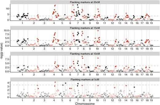
Identified makers using interval mapping with various flanking marker distances. Chosen markers are shown as gray vertical lines. Significant markers at the chromosome levels are shown in full color, nonsignificant markers at the chromosome level are translucent, the dashed line marks the whole genome significance threshold. Chromosomes are shown in alternating colors.
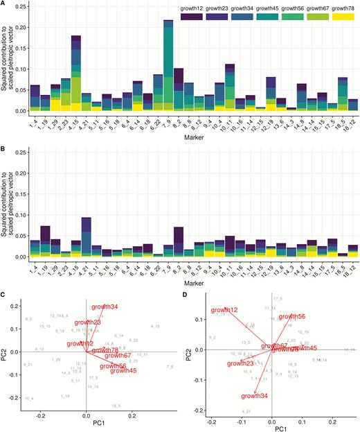
Pleiotropic effects of identified markers. (A) additive and (B) dominance contributions of the trait components to the final length of the pleiotropic vector. All trait contributions are scaled to trait standard deviation and are comparable. (C) additive and (D) (dominance): PCA of marker effects, arrows represent trait loadings in PC 1 and 2, marker IDs in gray are marker scores in PC 1 and 2. Markers are coded as chromosome and marker within chromosome, see Supplementary Material for genomic position.
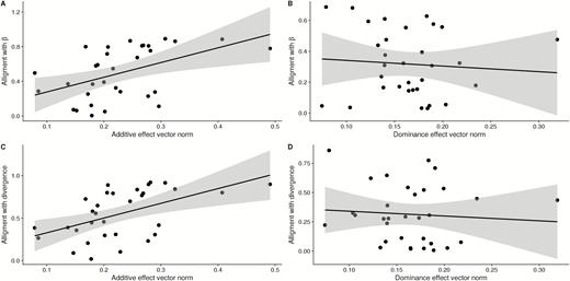
Size and alignment for chosen markers. Pleiotropic effect vector alignment with selection and divergence between founders. Panels A and B show the relation between pleiotropic effect vector norm and alignment to estimated selection gradient (), while panels C and D show the relation between pleiotropic effect vector norm and alignment to phenotypic divergence. (A and C) additive effects; (B and D) dominance effects.
Genome Prediction
Genome prediction produces pleiotropic effect vectors for all markers (Figure 5). We again see a widespread pattern of pleiotropy, but less so than in the mapped effects, as several of the large effect vectors have effects in only 1 or 2 traits. This is especially evident in the dominance effects. The PCA plot of marker effects confirms this, as the first 2 PCs are not related to early and late growth, as in the mapped markers, but combinations of single trait effects. We can also see the pattern of linkage affecting the pleiotropic vectors, as larger effects are often clustered and similar, suggesting that the regularization shrinkage prior was unable to pick a single marker as the best position for the effect, spreading the putative QTL over several neighboring markers [this is a known limitation of this type of sparsity inducing regression, see Piironen and Vehtari (2017)]. We can also see the pattern that larger additive effect vectors are more aligned with phenotypic divergence. Small effects, which where shrunken toward zero by the horseshoe prior, are essentially pointing in random directions, while larger additive vectors are more aligned with divergence and selection (alignment with divergence, slope = 2.42, P < 0.001; alignment with selection gradient, slope = 1.75, P < 0.001, Figure 6A,C). Dominance vectors again don’t have any pattern between magnitude and alignment (alignment with divergence, slope = −2.01, P = 0.09; alignment with selection gradient, slope = −2.14, P = 0.08, Figure 6B,D).
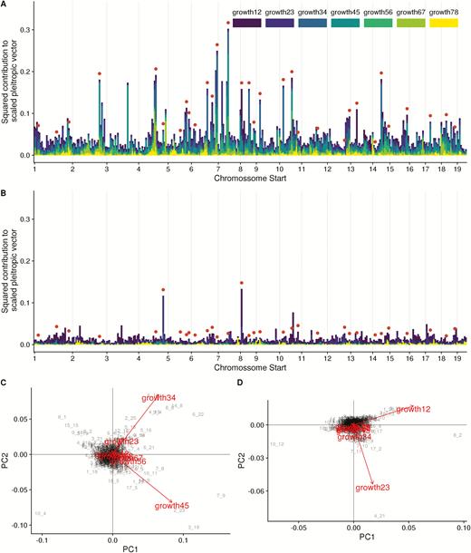
Regularized pleiotropic effects of all markers. (A) additive and (B) dominance contributions of the trait components to the final length of the pleiotropic vector. Significant markers in the QTL mapping are marked by the red dots. All trait contributions are scaled to trait standard deviation and are comparable. (C) Additive and (D) dominance PCA of marker effects, arrows represent trait loadings in PC1 and PC2, marker IDs in gray are marker scores in PC 1 and 2.
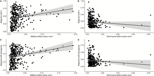
Regularized pleiotropic effect vector alignment with selection gradient and divergence between founders. Panels A and B show the relation between regularized pleiotropic effect vector norm and alignment to estimated selection gradient (), while panels C and D show the relation between pleiotropic effect vector norm and alignment to phenotypic divergence. (A and C) additive effects; (B and D) dominance effects.
Ancestral Predictions
Both regression models do well at predicting the phenotypes of the founder strains using only genetic effects estimated from the F3 generation (Figure 7). The genome prediction method is slightly better on the average prediction, but most ancestral growth periods are inside the posterior distribution (gray lines) for both models. First week of growth is somewhat anomalous in that the F3 generation is not intermediate to the two founders, possibly due to environmental effects, and so the prediction is poor. Growth in week 4 in the large strain is larger than predicted from the F3 genetic effects, suggesting either nondetected effects in the F3 or some other nonadditive genetic or environmental effects. The same applies to the week 7 growth, where both large and small strains are more different from the F3 then expected from the F3 additive effects.
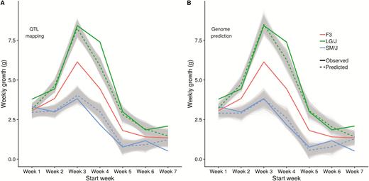
Ancestral predictions from additive effects. Predictions of the ancestral growth curves using additive effects estimated in the F3 generation. Solid lines are the observed growth curves, dashed lines the predicted growth curves from the 2 models. (A) QTL mapping of significant markers, (B) Genome prediction using all markers. Gray lines represent the posterior distribution of ancestral predictions derived from the Bayesian effect estimates.
Covariance Matrix Predictions
Genetic correlation matrices estimated from the pleiotropic effects from the mapped markers are broadly similar to the family level full-sib genetic matrix estimated from the mixed model fit. We can see the same strong correlation between late growth, and the positive correlation between weeks 2 and 3. The negative correlation between weeks 2 and 4 is present, but much smaller in magnitude in the QTL estimated matrix. The smallest correlations are between the early and late traits. Regressing the full-sib genetic matrix onto the genetic covariances predicted from the mapped markers (given by the sum of half the additive genetic matrix with one quarter of the dominance genetic matrix) reveals that the observed covariances are in general much larger than the predicted ones, but the pattern of covariances is similar (intercept = −0.01, slope = 2.43, P < 0.001). The outliers in the regression are the negative covariance between weeks 2 and 4 and the much larger observed variance in week 4. This is not surprising, since the full-sib genetic includes other sources of covariation, like maternal and common environmental effects. The genome prediction fared much worse, predicting variances and covariances close to zero for almost all traits (Supplementary Figure S3). Matrix comparisons can be seen in Table 2. The most similar matrices are the QTL mapping maker genetic matrix, followed by the QTL mapping marker additive genetic matrix. Both show high similarities in random skewers, Mantel matrix correlation, and a high proportion of shared subspace. The dominance matrix shows a relatively low matrix correlation and the lowest Krzanowski shared subspace correlation, suggesting it is different in structure to the full-sib genetic matrix. Genome prediction matrices have very low, nonsignificant Mantel correlation values, reflecting the poor estimate of the G-matrix correlations. Random skewers comparisons are all relatively high and significant, with the exception of the genome prediction dominance matrix. This can be due to a relatively similar first principal component in all matrices.
Matrix comparisons of the QTL mapping and genome prediction marker-based matrices with the estimated full-sib genetic via random skewers, Mantel correlation, and Krzanowski shared subspace correlation
| Matrix | Similarity to family full-sib genetic matrix | ||
|---|---|---|---|
| Random skewers | Mantel correlation | Krzanowski correlation | |
| QTL mapping marker | 0.872 (P < 0.001) | 0.69 (P < 0.001) | 0.86 |
| Additive genetic matrix | |||
| QTL mapping marker | 0.85 (P = 0.005) | 0.49 (P = 0.01) | 0.62 |
| Dominance genetic matrix | |||
| QTL mapping marker | 0.89 (P < 0.001) | 0.70 (P = 0.002) | 0.86 |
| Genetic matrix (½ G + ¼ D) | |||
| Genome prediction marker | 0.82 (P = 0.007) | 0.09 (P = 0.28) | 0.78 |
| Additive genetic matrix | |||
| Genome prediction marker | 0.6 (P = 0.057) | 0.20 (P = 0.16) | 0.40 |
| Dominance genetic matrix | |||
| Genome prediction marker | 0.83 (P = 0.002) | 0.12 (P = 0.29) | 0.77 |
| Genetic matrix (½ G + ¼ D) |
Discussion
The interaction between selection and multivariate covariation is a central part of our understanding of evolution. Even simple selection regimes can produce complex multivariate responses due to cascading developmental effects and genetic constraints. Here, we use a cross between two artificially selected lines of mice to investigate the genetic architecture of the multivariate response due to artificial selection. The target of selection in both lines was individual final weight, in opposite directions, and we use the various phases of growth as a model of a multivariate trait altered by selection. Using multivariate QTL mapping and genomic regression, we were able to map loci involved in the variation of growth and to simultaneously estimate vectors of genetic effects responsible for the variation in growth. Combining these effect vectors with quantitative genetics theory, we were able to directly link the pattern of pleiotropy and the genetic covariation of these traits.
As expected by the behavior of the phenotypes in the cross (Cheverud et al. 1996), most of the divergence between large and small is due to additive effects. The mean additive effect vector is practically collinear with the direction of divergence between lines, and we see a relation between the total size of the additive effects and the alignment with selection and divergence. This relation between alignment and size reflects the effect of selection removing large effects in other directions, that is, the larger the pleiotropic effect the more it must conform to the direction of selection to be maintained, while smaller effects can be less aligned with selection and still contribute to the divergence between lines. This clear alignment is absent from the dominance effect vectors, as the mean dominance vector has a low correlation with the phenotypic divergence and the direction of selection, and the size of the individual marker effects also has no bearing on their alignment to divergence and selection. Dominance vectors are not expected to contribute to the phenotypic divergence, since they are an interaction effect between alleles from the two founder lines, and so are only present in the crosses. These relations between effect size and alignment are present in both QTL mapping and genome prediction estimates of the additive and dominance effect vectors, but in the genome prediction the relations are much less clear when we look at the very small vectors. These small effect vectors are distributed in all directions but have very small norms (which is a measure of the overall effect of the locus across traits). Presumably, this is indicative that they have a negligible effect on the phenotype and are being shrunk to zero by the regularizing regression priors, and so the individual vector directions are essentially random.
Ancestral predictions using QTL mapping is surprisingly accurate, and most of the ancestral traits are within the posterior distribution of ancestral estimates, even though we are using only a small number of large effect QTL in the prediction model. The genome prediction analysis using sparse regression, on the other hand, is potentially including a number of small effects that do not meet a significance threshold, and so are excluded from the QTL mapping analysis. The inclusion of these many small effects have been proposed as a solution to the missing heritability problem (Bloom et al. 2013), and modern sparse regression and genomic prediction methods provide a promising framework for working with high density marker datasets (Pong-Wong 2014). Indeed, the sparse regression produces very good out-of-sample predictive performance when used to predict the phenotypes of the founder lines (Figure 7). Mapping could also be done in this sparse regression framework using variable selection, and the model displays reasonable agreement with the QTL mapping, producing large effect estimates that are close to the detected QTL (Figure 5). Furthermore, our analysis was done in standard generic Bayesian model fitting software (admittedly this was only possible since our maker data set is relatively small, but further advances in general statistical software should make using similar approaches in larger datasets possible). QTL mapping, on the other hand, provides us with a small set of interpretable pleiotropic vectors, which capture the modular aspects of early and late development, and can be used to understand the pattern of covariation that we see in the G-matrix. While the inclusion of all the marker helps with the ancestral prediction and uses effects that are ignored by the QTL mapping, using all of the markers for the estimation of expected covariances seems to be much more susceptible to noise introduced by small effect markers than the mean ancestral predictions, and the marker estimated variances and covariances using genome prediction are all close to zero. Some sort of variable selection would be necessary to make this estimate reliable using the genome prediction estimates. We do not pursue this further, but presumably even gradual removal of small effects would improve this estimate.
Using the pleiotropic effect vectors estimated in the QTL mapping analysis and quantitative genetics theory (Kelly 2009), we were able to construct expected additive and dominance genetic covariance matrices. The additive marker matrix is broadly similar to the observed full-sib genetic matrix, with strong positive correlations between the late traits, a strong correlation between weeks 2 and 3, and weaker correlations between early and late traits. The dominance matrix is different, with weak positive correlations within early and late traits and negative correlations between them. This clean separation between additive and dominance components of the G-matrix is difficult to achieve using only breeding experiments, and underscores how different these genetic effects can potentially be. The difference in the patterns of additive and dominance covariation suggests that these patterns have considerable latitude to vary and do not arise from a fundamental property of the system. If all gene effects on growth were constrained (i.e., the possible pattern of their effects were limited) by some set of developmental pathways, we would expect all sources of genetic covariation to share a similar pattern, reflecting the developmental constraints. (For example, a trade-off could restrict a locus with positive effects on trait A to have negative effects on trait B regardless of the effects being additive or dominant). The genetic matrix, composed of a one-half the additive matrix plus one-quarter the dominance matrix is similar to the full-sib matrix, but with smaller variances throughout. The negative correlation between weeks 2 and 4 is present, but not significant, in the marker estimated matrix (Figure 8C). Given that our maker-based estimates does not include several components that are expected to contribute to the genetic matrix, like shared environment and maternal effects, it is not surprising that the marker estimated variances are smaller than the observed genetic covariances. The smaller variances and covariances in the QTL mapping maker-based genetic matrix can also be attributed to the inclusion of only part of the direct genetic effects, since only loci with larger effects are used. Nevertheless, the general structure of the full-sib genetic matrix is captured by the expected covariance due to pleiotropy and linkage of the mapped loci, as we can see in the high values of matrix similarity and in Figure 8. The success in predicting the pattern covariation directly from pleiotropic effects underscores the importance of pleiotropy in determining genetic covariation, and suggests that a relatively small number of medium and large effect loci can be responsible for a large portion of the genetic constraints (which are captured in the pattern of trait covariation). Another possibility is that the distribution of pleiotropic effects is shared between small and large effects, either due to mutation, selection bias, or both. This shared distribution would explain why the general pattern of covariation, but not the total amount, is successfully predicted from a small number of markers.
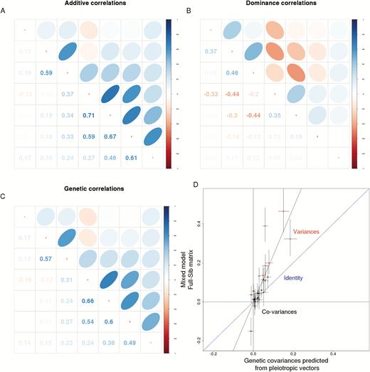
Additive, dominance, and genetic matrices. Estimated correlation matrices from QTL mapping marker effects. (A) Additive, G, (B) dominance, D (C) Genetic, ½ G + ¼ D. (D) Regression of genetic variances and covariances estimated from full-sib mixed model and estimated from markers. Error bars represent 95% posterior credibility intervals. Marker covariances are about half of observed covariances.
The distribution of pleiotropic effects in the QTL mapping analysis offers some insights into the genetic architecture of growth. First, we see that the full distribution of additive pleiotropic effects spans a modular variational space, with independent principal components aligned with the two stages of growth, early and late. This is somewhat unexpected given that the vector of selection on growth was in the direction of coordinated change in all phases of growth (Table 1), either increasing or decreasing the target of selection, week 9 weight. Given this target of selection, we would expect the distribution of the additive effects responsible for the divergence between large and small to be wholly aligned with the coordinated change of all growth phases, either increasing or decreasing all phases of growth. Indeed, on average, the additive effects are aligned with divergence, and large effects more so, but we still maintain a number of pleiotropic vectors with antagonistic effects in both phases, either increasing early traits and decreasing late traits or vice-versa (markers on the top-left and bottom-right quadrant of Figure 3C). The maintenance of this modular variation in pleiotropic effects could be associated with developmental or mutational constraints that limit the possible patterns of additive genetic effects. But, if this were the case, we might expect the dominance effects, which are not shaped by the selective history of the founders, to have a similar modular pattern. While the dominance effects PCA does not show the same clear early-late separation in orthogonal directions that we see in the additive effects, the dominance genetic matrix has a different distinction between early and late, with positive correlations within each phase and negative correlations between. So perhaps the modular aspect of the genetic effects can manifest in different ways. Additionally, the variational modularity between early and late growth that we see in the G-matrix is not only due to markers having modular effects, restricted to one stage of growth or another (markers close to the x and y axis in Figure 3C), but is also due to a combination of markers that have general effects in both stages (markers along the main diagonal, in top-right and bottom-left quadrants in Figure 3C) or the previously mentioned markers with antagonist effect in both stages. This reinforces the idea that there are several genotype–phenotype maps that can generate a modular covariance matrix (Pavlicev and Hansen 2011). However, several studies have found very low levels of antagonistic pleiotropy and many more modular pleiotropic effects in morphological traits (Leamy et al. 1999, 2002; Kenney-Hunt et al. 2008), suggesting that perhaps the specific genetic architecture underlying modularity could vary depending on the type of trait and on its evolutionary history. It is also possible that these patterns actually reflect some contribution of LD, since we are unable to reliably distinguish pleiotropy from LD because of the limited level of recombination in an F3 population. Therefore, application of our framework to an advanced intercross population or an outbred population would potentially provide even stronger insights because the lower levels of LD would allow for the clear separation of LD from pleiotropy.
The explicit link between genetic effects and covariation is a natural way to study multivariate evolution, but still rare in the literature (Kelly 2009). Using this approach, we were able to decompose the full-sib genetic matrix into its additive and dominance components. These components show different patterns of covariation, a consequence of the differences in the additive and dominance distributions of pleiotropic effects. While both classes of genetic effects show some signal of the division between early and late growth, the modular pattern is much more obvious in the additive effects. The full-sib covariance matrix, a common proxy for the additive genetic covariance matrix, is similar to the purely additive genetic matrix, but could differ more depending on the dominance component. Furthermore, we were able to accurately reconstruct the ancestral states in the founders using only the effects estimated in the F3 population, and this prediction was improved using all the markers in a sparse genome prediction model.
Funding
This work was supported by the Fundação de Amparo à Pesquisa do Estado de São Paulo (FAPESP; 2014/26262-4 and 2015/21811-2 to D.M.; 2011/14295-7 and 2013/50402-8 to G.M.), the U.K. Biotechnology and Biological Sciences Research Council (BBSRC; BB/L002604/1 and BB/M01035X/1 to J.B.W.), and the University of Bath through the Future Research Leaders Incubator Scheme to D.M.
Acknowledgments
We thank Jim Cheverud and John Hunt for insightful discussions that contributed to this work, Steve Chenoweth for discussions that were critical for the development of the analytical framework, Monique Simon for comments on the manuscript, and Anne Bronikowski for organizing and for inviting us to contribute to this special issue of Journal of Heredity.
