


Abstract
For the petrophysics model of tight sandstones, the elastic modulus of their sandstone and mudstone components are often substituted with those of quartz and clay, which affects model accuracy. To solve this problem, we innovate an adaptive approach for model the rock physics characteristics of tight sandstone. First, based on the relationship between P- and S-wave velocities from well logs and the elastic modulus of the rocks, the equivalent elastic modulus of tight sandstone under saturated conditions is calculated. Next, The Lee model and the Gassmann equation were jointly used to determine the equivalent elasticity modulus of tight sandstone matrix. The upper and lower limits of the equivalent elasticity modulus for mudstone and sandstone are established using the mudstone content curve, the least-squares method and the Voigt–Reuss–Hill (VRH) model. We used the random-walk algorithm to accurately calculate the equivalent elastic modulus of the sandstone and mudstone components. Finally, using the accurately obtained elastic modulus of sandstone and mudstone, the equivalent elastic modulus of the matrix is calculated. The Kuster–Toksöz model is subsequently applied to compute the dry-frame bulk modulus and shear modulus of the rock. Following this, the Brie model is used to calculate the elastic modulus of the mixed fluid, thereby completing the construction of the rock physics model for the study area. The results demonstrate that our improved petrophysics model can predict the S-wave velocity curve with ≤15% errors relative to the true curve. When sweet spot prediction was performed using reservoir-sensitive parameter (Vp/Vs) derived from the petrophysics template, the agreement between the predictions and well-log data was 80%. Thus, our petrophysics model method can be used to predict tight gas reservoirs effectively and will aid efforts to improve petroleum exploration works in the study area.
1. Introduction
Advances in the exploration and development of petroleum resources have caused exploration efforts to gradually shift toward unconventional reservoirs (Du et al. 2022). Tight sandstone reservoirs have attracted much attention as they are currently one of the most important type of unconventional reservoirs (McGlade et al. 2013; Szabó et al. 2022; Zhao et al. 2023). Unlike conventional sandstone reservoirs, tight sandstone is characterized by stronger heterogeneity, complex pore structure, and lower porosity and permeability (Desbois et al. 2011; Guo et al. 2016; Hu et al. 2023). Therefore, in petrophysical experiments, logging interpretation, or seismic inversion, it is difficult to effectively resolve the issues of tight sandstone using conventional sandstone rock physics models. To address this issue, many studies have been performed on the petrophysics modeling of tight sandstone reservoirs.
Nur et al. (1998) proposed a model based on critical porosity that relates the porosity of tight sandstones to their dry-frame and matrix velocities. Lee (2005) modified the consolidation parameter proposed by Pride to predict the elastic wave velocities of tight sandstones in various water saturation levels. Bosch et al. (2009) combined the Thomsen theory, Gassmann equation, and Lee porous media model to construct a petrophysics model suitable for tight sandstone reservoirs in their study area. Smith et al. (2009) applied the Kuster–Toksöz (KT) model to tight sandstone reservoirs to study how pore geometry affects rock elasticity. To handle the heterogeneity of tight gas reservoirs, Goodway et al. (2010) combined rock mechanics, petrophysical model, and AVO methods to predict the reservoir. P- and S-wave velocities in a real work area were successfully predicted using two different petrophysical models for the rock elastic modulus, which Ruiz & Azizov (2011a) proposed after studying how the elastic modulus changes with pore stiffness (Ruiz & Cheng 2010; Ruiz & Azizov 2011a; Ruiz & Azizov 2011b). Avseth et al. (2014) combined granular medium contact theory with inclusion-based model to construct petrophysical templates that consider the complex burial history of tight sandstone. In tight sandstone reservoirs, Wang & Wu (2015) proposed a self-consistent approximation-based soft-solid grain and soft-pore model that accounts for the effects of pore geometry and solid grains on rock velocities and predicted S-wave velocities. Based on the characteristics of tight sandstone reservoirs, Yin & Liu (2016) developed a petrophysical model that can characterize the crack-induced anisotropy of the reservoirs. To identify pore fluids, Sun et al. (2016) created a novel petrophysical model known as the tight sandstone double porosity model. Two methods for identifying pore fluids were proposed based on this model. According to the Xu–White model, Yang et al. (2018) used the porosity and P-wave velocities of tight sandstones to constrain the pore aspect ratios of sandstones and mudstones at different depths, thus, creating a more accurate version of the Xu–White model. Azadpour et al. (2020) combined the Xu and Payne models in tight sandstone reservoirs, and completed the prediction of S-wave velocities by modifying the Gassmann fluid equivalent model and introducing the C-factor index. Ba et al. (2021) established a petrophysical model of tight sandstone based on self-consistent approximation and differential equivalent medium theory, and used this model to study the brittleness properties dependent on mineral composition, porosity, and microcrack properties. Zhou et al. (2022) combined a dual-connected pore model with a linear sliding model to better characterize tight sandstone reservoirs, enabling the improved petrophysical model to more effectively extract microscopic reservoir information hidden in logging data. Wang et al. (2022) took into account the fluid pressure ratio between fractures and stiff pores to present a new inclusion-based petrophysical model of tight sandstone. The proposed model offered reasonable fluid information and aided in highlighting the variations between various pores. Durrani et al. (2023) used an inclusion-based petrophysics model to estimate the elastic characteristics of tight sandstones based on changes in pore aspect ratio. Zhang et al. (2024) proposed a petrophysical model based on variable critical porosity, and used this model to further analyze the influence of changes in reservoir petrophysical parameters on the P- and S-wave velocities. These developments in petrophysics models have significantly advanced the model of rock physics in tight sandstones.
In equivalent medium theory (EMT), the matrix is a critical element of the rock, as it influences the determination of the elastic modulus of the dried rock and the fluid replacement of the rock. It is customary to use the volume of the mineral components and their elastic modulus to calculate the equivalent elasticity modulus of the rock matrix. In practice, it is challenging to determine the mineral components of the rock, and this is especially true in tight sandstones. According to petrophysics theories, the mineral components of tight sandstones are often divided into sandstone and mudstone components, whose elastic modulus are then equated to those of quartz and clay. However, this approach can result in large errors, because the sandstone component often contains high percentages of feldspar and calcite, which can have a pronounced influence on the elastic modulus, in addition to quartz. Likewise, the mudstone component can include clay minerals such as kaolin and illite, which make it difficult to accurately approximate the elastic modulus of the mudstone component using a fixed number. Furthermore, the mineral elastic modulus used in EMT are usually derived from experiments, which cannot perfectly mimic the actual geological conditions of the study area. Thus, these moduli are intrinsically inaccurate. To build a more precise petrophysics model for tight sandstone, we suggest an adaptive technique for determining the equivalent elasticity modulus of the mudstone and sandstone components. In addition, a petrophysics template was created and cross-plot analysis was used to identify reservoir-sensitive elasticity parameters. The target stratum “sweet spots” were then precisely predicted using the sensitive parameter. The results of this investigation will be used as a guide for further research projects in tight gas blocks of a similar nature.
2. Methods and principles
2.1. Estimating the equivalent elasticity modulus of the tight sandstone matrix
The equivalent elasticity modulus of the matrix must be known to estimate the equivalent elasticity modulus of the mineral components in tight sandstone. The well-log data were used as the primary initial data for the inverse calculation in this study. If the rock is isotropic and fully elastic, the P- and S-wave velocities of a saturated rock are related to its bulk and shear modulus, as demonstrated by
where
These equations can be reformulated as shown:
After obtaining the equivalent elasticity modulus of saturated tight sandstone, the next step was to use a rock-frame model and Gassmann equation to calculate the equivalent elasticity modulus of the matrix. In selecting rock-frame models, empirical rock-frame models are widely used due to their strong applicability and low computational cost. Two common empirical rock-frame models are shown in Table 1. Based on the Pride model, the Lee model enhances the calculation formula of the shear modulus, thereby extending the applicability of the revised formula to a broader range of conditions. Therefore, the equivalent elasticity modulus of the tight sandstone matrix was determined to use the Lee model in this study.
Rock-frame models.
| Rock-frame model | Bulk modulus | Shear modulus | Parameterization |
|---|---|---|---|
| Pride model | Coefficient of consolidation, c | ||
| Lee model | γ factor |
| Rock-frame model | Bulk modulus | Shear modulus | Parameterization |
|---|---|---|---|
| Pride model | Coefficient of consolidation, c | ||
| Lee model | γ factor |
First, the shear modulus of the tight sandstone matrix was calculated. The result is unaffected by pore fluids at low frequencies and can be expressed as
where the shear modulus of the dry frame is represented by
The tight sandstone shear modulus matrix can be obtained using the Lee model:
where
To determine the bulk modulus of the tight sandstone matrix, the Lee model was substituted into the Gassmann equation (Equations 8 and 9). The incorporation of the Lee model transforms the Gassmann equation into a quadratic equation (Equation 10), which depends only on the bulk modulus of rock matrix. In Equation (10),
where
2.2. Random-walk algorithm for determining the equivalent elasticity modulus of the mineral components
The VRH model provides a wider range of equivalent elasticity modulus than the Hashin–Shtrikman limits (Fig. 1). This wide range creates a large space for search and optimization by the random-walk algorithm, which is beneficial for the optimization process. Therefore, the VRH model was used to compute the range of equivalent elasticity modulus of the mineral components of tight sandstone.
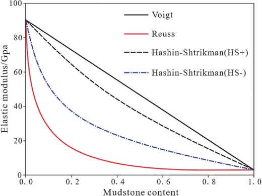
Limits of the VRH model and H–S bounds.
Initially, the Voigt model was employed to conduct correlation calculations on the upper limit of the equivalent elasticity modulus of the sandstone and mudstone. To achieve this, the Voigt model was reformulated as linear relations between mudstone content and the equivalent elasticity modulus of the matrix, as illustrated here:
where a and b are the gradient and intercept of the linear equation, respectively; the bulk moduli of the mudstone and sandstone are denoted by
Next, the correlation between the mudstone and sandstone lower limit of the equivalent elasticity modulus was determined using the Reuss model. The Reuss model can be reformulated as follows:
where the superscript R represents the elastic modulus derived from the Reuss model.
This method can determine the range of elastic modulus of the sandstone and mudstone components in tight sandstone. However, in practice, the relation between the mudstone content and the elastic modulus of the tight sandstone matrix is unlikely to be perfectly linear. Therefore, it is necessary to perform linear fitting on the obtained data. This paper employs the least-squares method for linear fitting. The least-squares method is a mathematical optimization technique that seeks the best function fit to data by minimizing the sum of the squares of the errors. This method can obtain the optimal value of the objective function, and can also be used for curve fitting to solve the regression problem. The formula is expressed as follows:
where S represents the sum of squared errors, yi represents the measured data, and y(xi) represents the function to be determined.
After obtaining the range of equivalent elasticity modulus of the mineral components, the random-walk algorithm was used to compute their exact equivalent elasticity modulus (Fig. 2). This algorithm works as follows: first, the algorithm gives a starting position, and then gets a new position after a random jump of a certain step length. The fitness of the new position is assessed by comparing the function values of the old and new ones, with the position having the smaller function value being chosen as the new position. Based on the new position, the function value is compared again after the random jump of the same step length. When a certain position still maintains the best fitness after reaching the specified number of iterations, the position is considered the optimal solution under this step length. Next, the step size is shortened and the calculation is repeated until the step size is reduced to the given control accuracy, so the obtained position can be considered the global optimal solution. The reliability of the optimal solution depends on the number of iterations and step length of the algorithm (Liu et al. 2017), and it has been shown that step length is more important than the number of iterations through many trials (Luo & Zhao 2006). Therefore, considering the computational cost, the usual method is to vary the step length to improve the predictive accuracy.
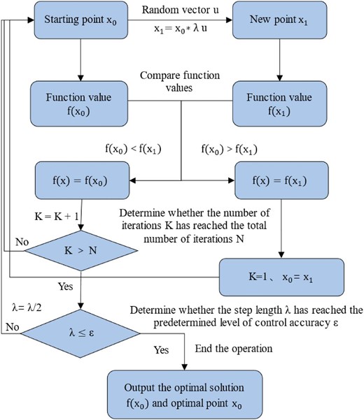
Flow of the random-walk algorithm.
Taking the process of determining the shear modulus for sandstone and mudstone as an example, the specific solution method is as follows: during the calculation process, the S-wave velocity is used as an effective parameter. The square of the difference between the S-wave velocities calculated from the shear modulus of sandstone and mudstone and the actual S-wave velocities is defined as the objective function (Equation 25), which is then optimized to find the solution. By this transformation, the calculation of the shear modulus of sandstone and mudstone is transformed into a global optimal problem of finding the minimum value of the objective function in a certain range:
where
2.3. Petrophysics model for tight sandstone
Based on the previous sections, we use the obtained density sandstone mineral component equivalent elastic modulus to build rock physical models. The modeling process is shown in Fig. 3, and the entire modeling work is based on the Xu–White model framework. The key links are shown next.
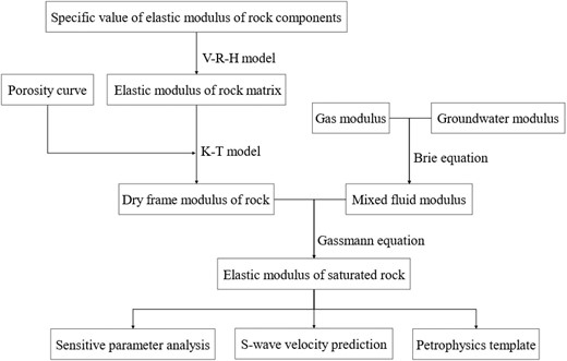
Petrophysical model process.
2.3.1. Calculating the equivalent elasticity modulus of the dry frame
The KT model, which is based on the first-order wave scattering approximation, establishes a relation between pore structure and rock elasticity parameters (Kuster & Toksöz 1974; Toksöz et al. 1976). After studying the mechanical properties of different pores, Berryman (1995) divided pores into sphere-, needle-, disk-, and coin-shaped, based on geometry and representing different stress states of rocks. Berryman, thus, obtained an improved KT model whose equations are as follows:
where
2.3.2. Calculating the equivalent elasticity modulus of mixed pore fluids
Based on experimental data, Brie et al. (1995) established relations between water saturation and the elastic modulus of the liquid and gaseous phases and introduced a water content exponent, e, which depends on the mixing between liquid and gas. The introduction of e improves the accuracy of the equivalent elasticity modulus (for mixed fluids) calculated by the Brie equation. The Brie equation can be written as follows:
where the gas and liquid bulk modulus are denoted by
By substituting this equivalent elasticity modulus into the Gassmann equations, the equivalent elasticity modulus of saturated tight sandstone can be obtained, thus completing the construction of the petrophysics model for tight sandstone.
3. Case study
3.1. Geological background of the research area
The study area is close to Jinxi flexural fold belt on the Yishan Slope of the Ordos Basin. The target stratum is the Shanxi Formation, which is composed of tight sandstone, coals, and mudstones. The tight sandstones consist of medium- and coarse-grained sandstones with diverse mineral components, which makes it difficult to ascertain the elastic modulus of their sandstone and mudstone components.
3.2. Calculating the equivalent elasticity modulus of the mineral components of the tight sandstone
Petrophysics analysis was performed via X-ray diffraction spectrometry on nine core samples from the study area to characterize the mineral components of tight sandstone in the target stratum. The results of whole-rock analysis are shown in Table 2.
Mineral components of the rock cores.
| Percentage content (%) | |||||||||
|---|---|---|---|---|---|---|---|---|---|
| Core no. | Type of rock | Quartz (Q) | Potassium feldspar (KF) | Calcite (Ca) | Dolomite (D) | Pyrite (P) | Siderite (L) | Ankerite (Ank) | Clay minerals (Clay) |
| 1 | Sandstone | 33 | 26 | 2 | 0 | 1 | 11 | 3 | 24 |
| 2 | Sandstone | 36 | 13 | 18 | 3 | 0 | 12 | 5 | 13 |
| 3 | Sandstone | 28 | 13 | 4 | 0 | 1 | 19 | 4 | 31 |
| 4 | Sandstone | 35 | 15 | 7 | 4 | 0 | 12 | 0 | 27 |
| 5 | Sandstone | 63 | 2 | 14 | 0 | 0 | 8 | 7 | 6 |
| 6 | Sandstone | 83 | 1 | 0 | 0 | 0 | 6 | 6 | 4 |
| 7 | Sandstone | 83 | 0 | 0 | 0 | 0 | 9 | 6 | 2 |
| 8 | Sandstone | 78 | 1 | 0 | 0 | 0 | 13 | 5 | 3 |
| 9 | Sandstone | 55 | 0 | 0 | 0 | 0 | 37 | 4 | 4 |
Table 2 shows that the quartz and clay contents vary substantially in the nine core samples. For example, Core 3 has a quartz content of 28%, whereas Cores 6 and 7 have quartz contents as high as 83%. Likewise, Core 7 has a clay content of only 2% (the lowest of the nine), whereas Core 3 has a clay content of 31%. Furthermore, some cores have higher percentages of minerals such as potassium feldspar, calcite, and siderite than the other cores. In a few cores, the sum of these minerals may exceed those of quartz or clay. Therefore, treating the sandstone and mudstone components as pure quartz and clay will result in substantial errors in elastic modulus calculations.
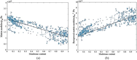
To improve the accuracy of the calculations, we initially employed the Gassmann relations and Lee model to determine the equivalent elasticity modulus of the matrix. We then extracted the upper and lower elasticity modulus limits of the sandstone and mudstone components from the mudstone content curve using the least-squares method and the VRH model. Figures 4 and 5 show the fitting graphs for the bulk and shear modulus of sandstones and mudstones under the Voigt model and Reuss model.
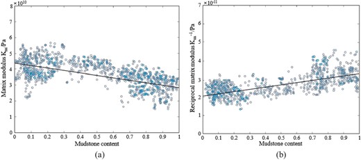
Fitting of bulk modulus using the Voigt and Reuss models. (a) Bulk modulus fitting of Voigt model. (b) Bulk modulus fitting of Reuss model.
Fitting of shear modulus using the Voigt and Reuss models. (a) Shear modulus fitting of Voigt model. (b) Shear modulus fitting of Reuss model.
As seen in Figs. 4 and 5, using the least-squares method to fit the data can achieve a good fitting effect. From the VRH model, it may be inferred that the fitting process provides a linear relation between certain coefficients and the equivalent elasticity modulus of the sandstone and mudstone components. Therefore, calculating the gradient (a) and intercept (b) of the linear relation provides the upper and lower limits for the equivalent elasticity modulus of the sandstone and mudstone components, respectively (Table 3).
Upper and lower limits for the equivalent elasticity modulus of the sandstone and mudstone components.
| Sandstone | Mudstone | |||
|---|---|---|---|---|
| Equivalent elastic modulus | Upper limits | Lower limits | Upper limits | Lower limits |
| Bulk modulus (GPa) | 36.2 | 35.1 | 32.1 | 29.9 |
| Shear modulus (GPa) | 26.5 | 25.8 | 13.4 | 10.9 |
| Sandstone | Mudstone | |||
|---|---|---|---|---|
| Equivalent elastic modulus | Upper limits | Lower limits | Upper limits | Lower limits |
| Bulk modulus (GPa) | 36.2 | 35.1 | 32.1 | 29.9 |
| Shear modulus (GPa) | 26.5 | 25.8 | 13.4 | 10.9 |
The equivalent elasticity modulus of the sandstone and mudstone components were subsequently accurately calculated using the acoustic-log curve and the random-walk algorithm. Table 4 contains the calculation's outcomes.
Calculated equivalent elasticity modulus of the sandstone and mudstone components.
| equivalent elasticity modulus | Sandstone | Mudstone |
|---|---|---|
| Bulk modulus (GPa) | 36.7 | 32.4 |
| Shear modulus (GPa) | 26.9 | 13.0 |
| equivalent elasticity modulus | Sandstone | Mudstone |
|---|---|---|
| Bulk modulus (GPa) | 36.7 | 32.4 |
| Shear modulus (GPa) | 26.9 | 13.0 |
Then, the equivalent elastic modulus of sandstone and mudstone was used to calculate the equivalent elastic modulus of the matrix, and it was compared with the actual measured values and the results calculated by the conventional model, as shown in Table 5.
Error analysis on the predicted equivalent elasticity modulus of the rock matrix.
| Core no. | Type of rock | Measured matrix modulus of the rock core (GPa) | Matrix modulus predicted by the conventional model (GPa) | Relative error (%) | Matrix modulus predicted by the proposed model (GPa) | Relative error (%) |
|---|---|---|---|---|---|---|
| 1 | Sandstone | 19.2 | 21.5 | 12.9 | 17.6 | 8.5 |
| 2 | Sandstone | 18.0 | 21.3 | 17.8 | 17.2 | 4.5 |
| 3 | Sandstone | 15.1 | 19.4 | 28.4 | 14.9 | 1.2 |
| 4 | Sandstone | 23.9 | 26.3 | 10.0 | 24.7 | 3.2 |
| 5 | Sandstone | 24.5 | 27.0 | 10.2 | 22.7 | 7.1 |
| 6 | Sandstone | 25.0 | 22.1 | 11.8 | 24.5 | 2.0 |
| 7 | Sandstone | 25.1 | 22.4 | 10.9 | 24.7 | 1.6 |
Considering actual measurements, the conventional model has an average error of 14.57%, whereas our improved model has an average error of 4.01% (Table 5). As our model predictions are much closer to the actual values, the model can be used to accurately predict the equivalent elasticity modulus of the tight sandstone matrix in the study area.
3.3. Application of the petrophysics model
3.3.1. Prediction of S-wave velocities using the petrophysics model
After obtaining the accurate equivalent elastic modulus of the tight sandstone matrix, a rock physics model was constructed based on the modeling approach described earlier. Figure 6 presents a comparative analysis of the S-wave velocities predictions between the improved model proposed in this study and conventional models.


Comparative analysis of S-wave velocities prediction with different models. (a) Well M1, (b) Well M2, (c) Well M3, and (d) Well M4.
The red and blue curves, respectively, represent the expected and measured S-wave velocity curves. The green curve indicates the relative error between the predictions and measurements. By analyzing Fig. 6, it can be found that the S-wave velocity curve predicted by conventional models generally has large errors, while the petrophysical model constructed in this paper is more consistent with the actual measurement results in terms of S-wave velocity prediction, and the relative error of the overall prediction curve is controlled within 15%. This demonstrates that the aforementioned model method not only accurately reflects the true rock physical characteristics of the target layer in the study area but also effectively corrects inaccuracies in shear wave velocity caused by wellbore collapse. Further, the data obtained using this method can be used for cross-plot analysis and the construction of petrophysics templates.
3.3.2. Sensitivity analysis of parameters
The selection of optimally sensitive parameters increases the accuracy and efficiency of reservoir prediction. Therefore, finding the rock elasticity parameters, which are sensitive to the presence of reservoirs, is an important part of rock physics model. By performing a cross-plot analysis between the available data and the petrophysics model, the elastic parameter that are sensitive to reservoirs can be identified. In this study, cross-plot analysis was performed using the Vp/Vs, S-wave acoustic impedance, and P-wave acoustic impedance. The results are shown in Figs. 7 and 8.
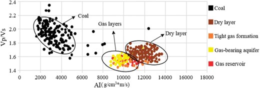
Cross-plot analysis between the Vp/Vs and P-wave acoustic impedance.
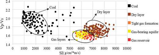
Cross-plot analysis between the Vp/Vs and S-wave acoustic impedance.
The cross-plot analyses on elasticity parameters obtained using our improved model can be used to differentiate reservoir strata (Figs. 7 and 8). For example, the coal in the figure as a whole is characterized by a high Vp/Vs values and low P-wave acoustic impedance and S-wave acoustic impedance, whereas sandstone strata have low Vp/Vs values and high P-wave acoustic impedance and S-wave acoustic impedance. Additionally, the dry layer of the sandstone exhibits higher Vp/Vs values than gas layers. Therefore, the Vp/Vs can serve as a sensitive elastic parameter for identifying gas reservoirs.
3.3.3. Construction of a petrophysics template
Based on the improved petrophysics model, we constructed a petrophysics template and obtained relations between P-wave acoustic impedance and Vp/Vs and porosity, mudstone content, and water saturation (Fig. 9).
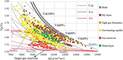
Petrophysics template for Vp/Vs and P-wave acoustic impedance.
The red, blue, and gray lines represent water saturation, porosity, and mudstone content, respectively. The division of reservoir range can be realized through the analysis of petrophysics template (Table 6). The target gas reservoir in the study area is primarily distributed within the following ranges: P-wave acoustic impedance of 8500 to 11 500 g/cm³·m/s, Vp/Vs ratio of 1.48 to 1.56, mudstone content of 3% to 35%, porosity of 6% to 12%, and water saturation of 40% to 65%. Using this range can provide a basis for reservoir prediction in the subsequent inversion process.
Elasticity parameter zones for reservoir strata.
| Reservoir type | P-wave acoustic impedance (g/cm3 m/s) | Vp/Vs | Water saturation (%) | Porosity (%) | Mudstone content (%) |
|---|---|---|---|---|---|
| Class I reservoir (gas strata) | 8500–11 100 | 1.48–1.56 | 40–50 | 8–12 | 3–10 |
| Class II reservoir (tight gas formation) | 9000–11 500 | 1.48–1.58 | 50–65 | 7–12 | 3–35 |
| Class III reservoir (gas-bearing aquifer and dry layer) | 8000–13 500 | 1.48–1.84 | >60 | 1–12 | 4–60 |
3.3.4. Prediction of sweet spots
Eight wells in the study area were used for sweet spot prediction, whereas five wells were used to validate the predictions. Figure 10 shows the sweet spot area of the target layer predicted by using the preferred reservoir-sensitive parameters. In the figure, the red area indicates the area with gas layer development (primary reservoir), the yellow area indicates the area with poor gas layer development (secondary reservoir), and the blue area indicates that there is no gas layer development (non-reservoir) in the area. The gas-bearing properties of the predicted area are verified by using the existing logging data. The results indicate that the gas-bearing properties of M1, M2, M3, and M4 wells are consistent with the well-log interpretation. The predictions were 80% consistent with the actual values, which shows a great predictive performance.
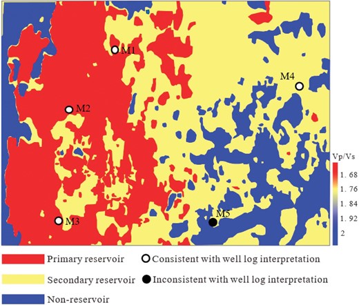
Sweet spot prediction in the target stratum.
4. Conclusion
Using the elastic modulus of sandstone and mudstone derived from the random-walk algorithm to calculate the elastic modulus of the rock matrix, the results reveal an average error of 4.01% compared to actual measurements. This relatively small error indicates that the calculated values are closer to the observed data. This method can effectively improve the calculation accuracy of elastic modulus of tight sandstone matrix in the study area.
Research results indicate that the improved rock physics model provides a good fit for the actual rock physics characteristics of the study area. Through cross-plot analysis and the construction of rock physics templates, Vp/Vs was identified as the elastic parameter most sensitive to gas layers. Additionally, the distribution range of elastic parameters for the main gas-bearing layers in the study area was determined.
When the sensitive parameters were used to predict sweet spots in the target stratum, the agreement between the ground truth and predictions was 80% (validation via well-log data). Therefore, the suggested approach can direct the investigation of tight gas reservoirs in the research region.
Conflict of interest statement
None declared.
Funding
This work was supported by fundamental research funds for the National Natural Science Foundation of China (grant no. 42474186), the central universities (grant no. 2023JCCXLX01) and Open Fund of State Key Laboratory of ‘Coal Resources and Safe Mining’ (grant no. SKLCRSM20KFA13).
Data availability
The data that support the findings of this study are available from the corresponding author, Suzhen Shi, upon reasonable request.
