


Abstract
This paper studies the effect of emigration on technological change in sending locations after one of the largest migration events in human history, the mass migration from Europe to the United States in the 19th century. To establish causality, we adopt an instrumental variable strategy that combines local growing-season frost shocks with proximity to emigration ports. Using data on patents, we find that emigration led to an increase in innovative activity in sending localities. Using data on capital and labor inputs in agriculture and industry, we find evidence of an increased capital intensity related to new technologies in both sectors. We argue that these results are consistent with theories of induced (labor-saving) innovation due to high labor costs following emigration.
A set of Teaching Slides to accompany this article are available online as Supplementary Data.
1. Introduction
Emigration is often depicted as a major problem for developing countries. However, by pushing up labor costs it may also spur technological advances. A long-standing hypothesis posits that high labor costs induce innovation and adoption of labor-saving technologies (Hicks 1932; Habakkuk 1962; Zeira 1998; Alesina, Battisti, and Zeira 2018). While others have argued that innovation may be discouraged (see e.g. Ricardo 1951; Kremer 1993), the effect of labor cost on technology depends on whether new technologies reduce labor requirements or not (Acemoglu 2010). Thus, the effect may vary over place and time, and ultimately becomes an empirical matter.
This paper investigates the long-term effects of emigration on technological change in sending communities. We do so in the context of Swedish mass emigration to the United States starting in the mid-19th century when as much as one quarter of the Swedish population crossed the Atlantic. At the onset of its transatlantic migration experience, Sweden was primarily an agrarian economy, abundant in low-wage work and labor-intensive production processes. Indeed, migrants were typically low-skilled, often working within the agricultural sector in the early phases of the migration episode. As a consequence, the cry for labor-saving technology was salient among contemporary observers (Fredholm 1879). During the next decades, Sweden underwent an industrial revolution with a vast increase in mechanized equipment and technological innovations (Heckscher 1941). At the turn of the century, patents had reached record high levels. This paper asks if and to what extent emigration played a role in this development.
To measure the effects of emigration on innovation, we use a novel and hand-collected data set covering the universe of patents in Sweden between the mid-19th century and World War I.1 In addition, we collect data on capital and labor inputs in agriculture and industry. We combine this with data covering all registered Swedish emigrants and immigrants in this period to construct a data set at the level of approximately 2,400 municipalities between 1867 and 1914.
Our main empirical framework compares economic outcomes between municipalities within the same region but with different emigration histories. To obtain exogenous variation in emigration 1867–1914, we employ an instrumental variable strategy that combines two sources of variation.2 First, we construct growing-season frost shocks 1864–1867 to capture the fact that poor harvests were a crucial push factor for the first wave of emigration in the late 1860s. Second, since there were two main emigration ports—Gothenburg and Malm—we captured the travel cost of emigration using a municipality’s proximity to its nearest emigration port. Interacting these two sources of variation, the idea behind the instrument is that negative shocks to agriculture increase emigration, especially when the travel cost is low.3 Because Swedish migration was highly path dependent, which we corroborate, we can strongly predict not only the first wave of migration, but also emigration during the entire mass migration period.
Our main result is that emigration causes a long-run increase in technological innovation in sending municipalities. Our preferred IV estimate indicates that a 10% increase in the number of emigrants 1867–1914 increases the number of patents by about 6% in the same period. The positive effect on patents is, in particular, driven by the upper tails of innovative activity (the intensive margin) rather than by municipalities entering into the innovation business (the extensive margin). Weighting patents by their economic value, we find a similarly strong and positive effect on innovation.
We proceed in several steps to investigate additional effects and mechanisms. In sum, we argue that the pattern of results is best explained by the induced innovation hypothesis, that is, that emigration raises labor costs and creates an incentive for adopting or inventing labor-saving technologies. In county-level data, we document a positive relationship between emigration and agricultural wages.4 Separating patents by sector, we also find that the labor-intensive agriculture and food sectors saw the largest increases in innovation, together with machinery.
To provide a closer examination of whether emigration exposure within a given sector increases innovation, we use data on emigrants’ prior occupations and match them to 89 patent classes. In regressions including municipality and patent-class fixed effects, we indeed find that patent classes that are more exposed to emigration also see more innovation. While this specification is not causally identified, our IV estimates suggest that OLS provides a lower bound on the effect of emigration on innovation. This setting also allows us to study spillover effects in two dimensions. First, we find that innovation within a class also increases with overall municipal emigration, even after controlling for class-specific emigration, consistent with our main IV results using variation at the municipality level. Second, we show that innovation responds to national emigration within the patent class as well, in line with inventors taking national trends into consideration.
We next turn to the effects of emigration on the agricultural and industrial sectors. In agriculture, we find that emigration causes a decrease in labor intensity as measured by the number of unskilled workers per draft animal. Draft animals per arable land also increased. These results suggest both a greater extent of mechanization and substitution away from labor. Studying the relative increase in draft animal use more closely, we find that horses, rather than oxen, drive this effect. We interpret this as an indication of technology adoption, as horses were essential for using the modern, productive tools of the time, such as mowing-machines, rakers, and binders (Morell 2011).
Next, we examine how emigration affected technology within the industrial sector. Consistent with models of labor-saving technological change (Zeira 1998), we find that emigration caused firms to increase their capital share, as measured by the ratio of machine power to output value. With data on incorporated firms, we also document an increase in equity per non-agricultural worker, further indicating an increase in capital intensity.
In terms of employment shares, we find a decrease in unskilled workers per capita in agriculture. In contrast, manual workers per capita increase in non-agricultural occupations. However, in line with technological advances, the ratio of high-skilled to low-skilled workers increases. Finally, we find that incorporated firms report higher profits per worker and that municipal tax incomes are greater, indicating that emigration led to increasing productivity and economic growth over time.
Lastly, we explore the potential that return flows from the United States affected innovation (cf. Borjas and Bratsberg 1996; Kerr 2008; Mayr and Peri 2008; Dustmann, Fadlon, and Weiss 2011). However, we do not find support for our results being driven by inventors with typical return migrant occupations or by innovation occurring in patent classes that are more common in the United States than Sweden. Moreover, in simple regressions, there is no association between return migration and innovation, conditional on emigration. These results together suggest that return migration and information flows from the United States are not the crucial mechanisms behind our results on innovation, although we cannot entirely rule out their potential influence.
In sum, the mass migration era had important effects on technological change in Sweden during the second industrial revolution. Our results are consistent with the classic hypothesis of induced innovation, with its origins in Hicks (1932) and later popularized by Habakkuk (1962) and Allen (2009). Zeira (1998) develops the theory formally. Acemoglu (2010) provides a comprehensive framework to analyze the relationship between labor scarcity, labor costs, and innovation, and concludes by calling for more empirical research.5
A few studies empirically investigate the effect of a change in the supply, or price, of an input on technological innovation and adoption (Popp 2002; Acemoglu and Finkelstein 2008; Lewis 2011; Hanlon 2015; Lafortune et al. 2015; Aghion et al. 2016; Lew and Cater 2018). In particular, some empirical studies link emigration to technological change in origin locations. Hornbeck and Naidu (2014) find increased technology adoption due to out-migration of low-wage labor after the Great Mississippi Flood of 1927. Clemens, Lewis, and Postel (2018) study the effect of the exclusion of Mexican agricultural workers on wages and technology adoption, while San (2022) looks at the effects on innovation. Two recent articles study the effect of reduced labor costs following an inflow of low-skilled labor, finding it lowers productivity and innovation (Imbert et al. 2020; Bustos et al. 2022).6
Through the empirical setting, our paper is also related to a growing body of economic studies of the Age of Mass Migration.7 While several studies focus on the effects of immigration on different aspects of the US economy, fewer studies explore the effects on the Old World.8 Boyer, Hatton, and O’Rourke (1994), O’Rourke and Williamson (1995), and Hatton and Williamson (1998) study the aggregate effect of emigration on labor markets at home in Ireland and Sweden, all finding that emigration increased real wages. Ljungberg (1997) finds that emigration was a major factor in the elevation of Swedish wages. O’Rourke (1991) finds that increasing labor costs led Irish agriculture to move away from tillage and increased mechanization. Karadja and Prawitz (2019) examine the effect of emigration on political development in Swedish municipalities and find that emigration substantially increased the membership in local labor organizations and, later, mobilized support for pro-labor parties. The findings in Karadja and Prawitz (2019) are consistent with the results in this study by providing a complementary channel—workers’ bargaining strength and labor unions—through which labor costs may have increased due to emigration. This study differs by evaluating the mechanism of induced innovation and doing so by using newly digitized data on patents, agricultural inputs, and manufacturing firms, as well as a within-municipality analysis.
The remainder of the paper proceeds as follows. Section 2 provides an overview of the historical background, while Section 3 describes our data. Section 4 introduces the econometric framework and discusses the first-stage relationship between our instrument and emigration. Section 5 presents the main results divided into three subsections: effects on innovation, on capital and labor intensity, as well as an evaluation of the role of return flows from the United States. Section 5.4 provides robustness tests, and Section 6 concludes the paper.
2. Historical Background
Mass Migration.
Nearly 30 million Europeans emigrated to the United States during the Age of Mass Migration (1850–1913). Along with Ireland, Norway, and Italy, Sweden had one of the highest sending rates in per capita terms (Taylor and Williamson 1997). About a quarter of the Swedish population emigrated, mostly to the United States. In total, almost 1.3 million Swedes emigrated between 1860 and 1913.
Sweden’s transatlantic emigration episode takes off in the last years of the 1860s, coinciding with a severe famine in large parts of the country. It is well-recognized that these so-called famine years were a key push factor behind the Swedish transatlantic mass migration (see e.g. Sundbärg 1913; Barton 1994; Beijbom 1995). The famine and the resulting poverty followed after a series of bad harvests due to bad weather conditions in the late 1860s. In particular, 1867 saw record-breaking cold temperatures during the growing season months.
Figure 1 depicts the yearly flow of emigrants. The initial rapid increase in emigration starting in 1867 is clearly visible in the figure. In the five years following 1867, as many as 150,000 Swedes, or 4% of the population, emigrated. This first wave of emigration was followed by a period of comparatively low emigration numbers before migration took off again during the first years of the 1880s. In the following decade, about half a million Swedes left the country during the most intense period of the Swedish transatlantic migration experience.
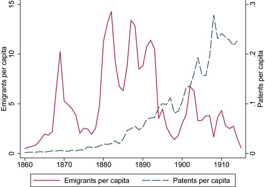
Aggregate national time series 1860–1914. This figure displays the aggregated yearly flows of emigrants and granted patents (with a patent holder or inventor residing in Sweden) per 1,000 inhabitants.
Social networks were crucial determinants of emigration. Apart from reducing transaction costs for later migrants upon arriving in the New World, migrants already in the United States sent pre-paid travel tickets back home. As many as every second emigrant is believed to have traveled on such tickets (see e.g. Runblom and Norman 1976; Beijbom 1995). Letters sent home from the United States were also common and often described the overseas experience in overly positive language. Among migrants from Scandinavia arriving in the United States in 1908–1909, 93.6% stated that they were joining friends or relatives who had previously migrated (Hatton 1995). Online Appendix Figure B.1 displays the high positive correlation between the early wave of emigration during the period 1867–1874 and subsequent emigration during 1875–1914, confirming that there was strong path dependence in migration patterns.
Emigration, Labor, and Technology.
At the start of the Swedish migration episode, Sweden was a predominantly agrarian society. In 1860, almost 80% of the labor force worked in agriculture, as compared to about 10% in the industrial and manufacturing sectors (Edvinsson 2005). In the following decades, Sweden became increasingly industrialized. While the sources of this development remain disputed among economists and economic historians (e.g. Wicksell 1882; Sandberg 1979; O’Rourke and Williamson 1995; Ljungberg 1996), it is well established that Swedish real wages went from being below the Western European average in the 1860s to the level of their British counterparts by 1914.
As emigration reached new peaks at the turn of the century, the backlash from economic and political elites became more severe, to a large extent based on concerns about the adverse effect of labor scarcity on the Swedish economy (Kälvemark 1972). Following the start of the first wave of emigration at the end of the 1860s, Swedish wages saw a substantial increase. The typical emigrant in the first wave worked in agriculture, and it was also low-skilled agricultural wages that increased the most and came close to industrial wages (Jörberg 1972a). After a downturn, Swedish wages rapidly increased again starting in the latter part of the 1880s and continued to do so in the following decades. Other studies have found that emigration was a major reason behind this increase.9
An official government report on Swedish agriculture during 1871–1919 concluded that labor scarcity made a more extensive usage of agrarian machines necessary (Sjöström 1922). Similar sentiments are put forward in Moberg (1989), Gadd (2000), and Morell (2001). According to Moberg (1989), the emigration was partly responsible for inducing more mechanization since it “affected a particularly capable part of the labor force”. Together with a rapid increase in wages, this resulted in a large demand for agricultural machinery. Moberg (1989) emphasizes that even if machines also produced better quality than manual labor, it was the sudden shortage of labor that was the main reason for the increased demand. Morell (2001) points out that a significant part of the agricultural technology introduced after 1870 was labor saving. This was especially the case for technology related to harvesting, threshing and mowing, but also the introduction of bigger and better harrows and modern milking machines. According to Gadd (2000), harvesting and threshing machines reduced the use of manual labor by at least 60%.
While most emigrants came from the agricultural sector in the first two decades, the period after about 1890 saw an increase in emigrants stemming from the industrial sector. In the same period, Sweden underwent a rapid period of industrialization. It is important to note that Swedish industrialization did not only occur in urban areas. In fact, industries were predominantly located in rural areas, often in close proximity to natural resources (see e.g. Svennilson, Lundberg, and Bagge 1935; Heckscher 1941; Ljungberg 1996). There was consequently relatively high within-location labor mobility between the agricultural and industrial sector (Svennilson, Lundberg, and Bagge 1935). At the same time, many industries, such as the iron industry, were locally rooted and relied on local labor to a large extent (Heckscher 1941). According to Schön (2000), the increased labor mobility led to more competition for workers, and producers were forced to increase mechanization to decrease labor costs. In general, it was the new and more productive industrial businesses that could offer higher wages. In neighboring Norway, the emigration commission of 1912–1913 concluded that by contributing to the increase in wages, emigration had been instrumental in promoting the process of mechanization and rationalization of production (Hovde 1934).
The importance of labor-saving inventions constituted a focus for contemporary writers, as is clear from Fredholm (1879). In arguing for a patent law reform, Fredholm makes several comparisons between Sweden and the United States and argues that it was not enough to merely import the many labor-saving American innovations. Instead, Sweden needed its own innovations and industry. From initially low levels in the 1860s and 1870s, patents increased rapidly towards the last decade of the 19th century, as shown in Figure 1. Heckscher (1941) described the period as an era of technological revolution, noting that there was a vast increase in mechanized equipment. Gustaf de Laval’s milk separator constituted a major industrial breakthrough in the dairy industry, and Alexander Lagerman revolutionized the production of matches with his matchstick machine. Yet, many of the new innovations of the era were minor in terms of innovative contribution (Morell 2001). For instance, machine engineer Frans Thorén in Karlshamn invented a device for sugar mill diffusers that decreased the necessary number of workers by making it possible to close the bottom flap of the operator compartment above the machine. Karl Alberth invented a simple hay rack that was widely advertised as a labor-saving innovation.
Sweden implemented a rigorous system of technical examinations in 1885, similar to the American and German systems. This required a rigorous novelty search before a patent was granted, while patents were previously granted as long as certain administrative requirements were fulfilled. The vast majority of patents were filed by individuals and not by firms, suggesting that fixed costs were relatively low. Indeed, historians have termed the period as an “era of independent inventors” (Hughes 1988). However, to apply and receive patent protection for an invention, the applicant needed to pay both an application fee and a renewal fee. While the application fee was low during the main period of study, the Swedish renewal fees were increasing over the patent’s duration, thus rendering renewals relatively costly.10 This potentially leads independent inventors to sell patents to firms. From initially low levels, the market for buying and selling patents increased over the period (Andersson, Berger, and Prawitz 2021).
Yet a large share of inventions were made in response to local needs and demands. For example, noting the lack of a general system for high-precision gun and rifle manufacturing, C. E. Johansson invented his famous gauge blocks while working in the Royal weapons factory in Eskilstuna, one of Sweden’s centers for mechanical engineering at the time. A broader example is the large number of Swedish metallurgical inventions originating from the Bergslagen mining district, one of many examples being the hardness test method developed by J. A. Brinell while working as the head engineer at Fagersta Ironworks. Similarly, inventions connected to woodworking emerged disproportionally in the region of the Swedish Northeastern coast where the majority of sawmills were located.
3. Data
Our data are organized at the municipal level using administrative boundaries from 1863, which we define using an administrative map from the Swedish National Archives (Riksarkivet). To get consistent borders over time, we collapse urban municipalities with their adjacent rural municipalities or municipalities as these borders sometimes change due to urban expansion. In total, we observe nearly 2,400 municipalities. Below, we present the data sources in more detail.
Patents.
We digitized handwritten ledgers on patents from the Swedish National Archives and the archives of the Swedish Intellectual Property Office (PRV).11 The data set includes all Swedish patents granted between the mid-19th century and 1914 and specifies the year of application and grant, the names of all inventors and patentees, and their professions as well as their area of residence. There are a total of 18,250 registered patents with an inventor or patentee residing in Sweden during the period 1860–1914. About 90% locate one or more patentees in a specific city or municipality. For patents with multiple inventors living in different municipalities, we assign each municipality one patent each. Thus, our patent variable measures local involvement in granted patents.12 The final data set contains 17,179 such patent observations for the years 1860–1914. Figure 2 displays the spatial distribution of patents per 1,000 inhabitants. As reflected in the figure, while urban areas stood for a large share of patents, innovation was geographically widespread and common in rural areas as well.
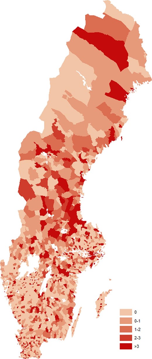
This figure displays the spatial distribution of the number of patents 1867–1914 per 1,000 inhabitants in 1865.
To get a measure of the quality or value of a particular patent, the literature typically uses either the number of citations received or the amount of patent fees paid by the owner to maintain the patent in force for a longer period of time. Unfortunately, citation counts are not available in our sample period. While citations are considered to be a good indicator of the innovative quality of a patent, renewal fees are a more suitable measure of the economic value of patents. This is because the patentee has to make the renewal decision each year based on the expected economic return from extending the patent right (see e.g. Schankerman and Pakes 1986; Burhop 2010). We use the number of years that a patent is in force as a proxy for its economic value.
Capital and Labor.
Data on capital inputs in agriculture and industry are digitized from publications and handwritten ledgers from Statistics Sweden.13 The agricultural data was originally collected by local authorities at the parish level, which we digitizeed and linked to the municipality level, and covered all parishes without town privileges in 1910. In particular, we obtain data on the use of draft animals, distinguishing between horses and oxen. The industrial data originate in firm censuses covering all Swedish manufacturing firms in 1900 and include detailed information on the placename, which we spatially link to our municipalities. We obtain data on output value and the amount of power generated (measured in horsepower).
Data on all incorporated firms and their profits 1901–1919 are obtained from the Swedish Companies Registration Office.14
To characterize local labor markets by sector and skill, we use full-count decennial census data between 1880 and 1910 from the National Archives of Sweden and the North Atlantic Population Project.
Yearly data on unskilled wages in the agricultural sector, so-called daywages, at the county level are from Jörberg (1972b). Their employment terms resembled those of industrial and construction workers (Enflo, Lundh, and Prado 2014), and they are considered to reflect the level of cash wages for other unskilled trades as well, for example, within the industrial sector (Ljungberg 1997). We construct real wages by deflating the nominal wage series with a regional foodstuff index consisting of 14 food items obtained from Jörberg (1972a).
Migration.
We measure migration using two independent sources. The first is collected by priests at the parish level and later digitized by genealogists from parish church books.15 Variables include migration date, age, gender, and occupation. We link migrants in each parish to a municipality. In addition, we use data from passenger lists compiled by shipping companies starting in 1869. Apart from the variables available in the church records, this additional data set includes the port of exit, giving us information on which routes emigrants used when migrating. Although these two data sets are independent, they are highly correlated, as shown in Karadja and Prawitz (2019). Consistent with historical evidence (Runblom and Norman 1976), this suggests that most emigrants migrated directly from their home parishes rather than migrating within the country before leaving Sweden.
One potential concern is mismeasurement in migration, in particular, unregistered emigration before the Emigration Ordinance of 1884, which introduced stricter requirements for emigrant agents to record migrants (see e.g. Bohlin and Eurenius 2010). To decrease the extent of unreported emigration in the parish records, we aggregate both emigration data sets to the municipality-year level and choose the maximum of the two numbers for any given year as our measure of emigration.16 In Online Appendix Table A.21, we show that our results are robust when using only the passenger data or the parish church books, as well as using emigration only after the Emigration Ordinance. In Online Appendix A.3, we discuss potential bias related to measurement error further.
Weather.
Daily temperature data are provided by the Swedish Meteorological and Hydrological Institute (SMHI) as well as the Norwegian Meteorological Institute (MET). For the period between 1864 and 1867, which we use to construct our instrumental variable, there are 32 available weather stations.17 While the relatively few number of stations may reduce precision, this should pose less of a problem when studying temperature as compared to rainfall, since temperature is more evenly distributed in space, especially in the Northern hemisphere. Moreover, we exploit deviations in temperature from long-term means, which are known to be more reliable for spatial interpolation than temperature levels (Hansen and Lebedeff 1987). More details on how we use these data are provided in Section 4.
Additional Data Sources.
We use several other data sources to obtain baseline control variables. Soil suitability data for different agricultural produce (barley, oats, wheat, livestock, and forestry) are taken from the FAO GAEZ database. Railway data are from the National Archives of Sweden. Population data for 1865 are from Palm (2000) and complemented with data from the National Archives of Sweden.
4. Empirical Framework
To measure the long-run effects of emigration on innovation, we instrument for emigration using a measure of push factors occurring before the start of mass migration. The instrument is the interaction between growing-season frost shocks in 1864–1867 and a municipality’s proximity to an emigration port. Online Appendix C.2 provides a more detailed description of the identification strategy, the construction of frost shocks, as well as several validation tests. Figure 3 displays a map of the spatial distribution of growing season frost shocks 1864–1867.
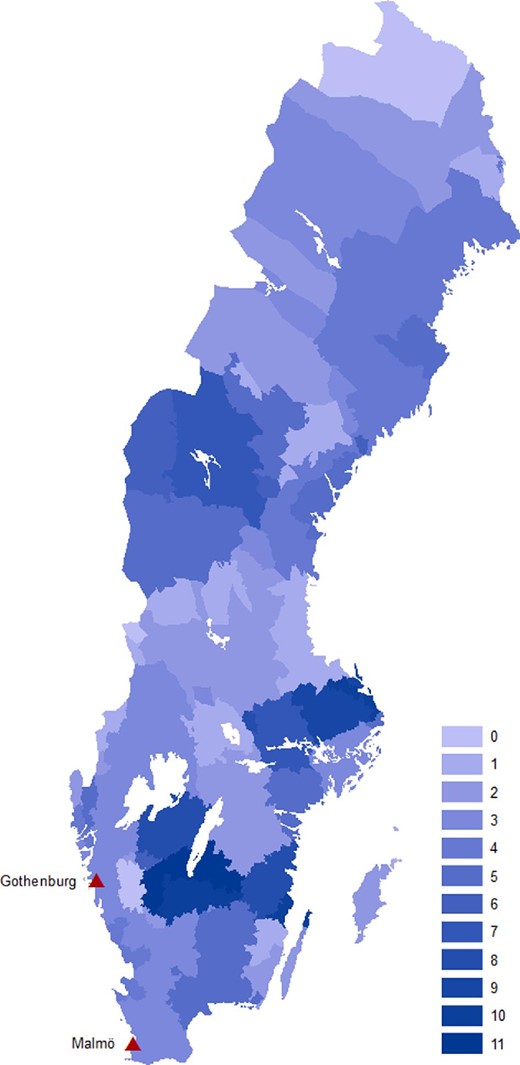
This figure displays the spatial distribution of the number of growing season frost shocks in 1864–1867. The triangles mark the two main emigration ports, Gothenburg and Malmö.
The log of population in 1865 is always included in |${\bf X}_{ic}$| to scale the effects to initial population levels. In addition, |${\bf X}_{ic}$| includes the proximity to the nearest town, trade port, railway, and weather station, and to Stockholm, the log municipality area, log length of the growing season, latitude and longitude, share of arable land, indicators for urban municipalities and for having at least one patent 1860–1864, log number of firms 1865, and the log power per unit of output 1865, as well as a set of indicator variables for high soil quality for the production of barley, oats, wheat, livestock, and timber.22 To control for the fact that regions may differ in several unobserved dimensions, we also include a set of county fixed effects (|$\alpha _{c}$| and |$\theta _c$|). Thus, we only compare municipalities within smaller regions.23 The error terms capture all omitted influences.
We use standard errors that are cluster robust at the level of the 32 weather stations. To supplement this baseline, we provide standard errors calculated using other methods in Section 5.4. This includes clustering at the county level as well as using wild-t cluster bootstrap and spatially robust errors in a radius of up to 200 km following Conley (1999).
4.1. First Stage Results
Table 1 displays the effect of the instrument on total emigration during the mass migration period 1867–1914. In column (1), the coefficient of 0.064 indicates that a one standard deviation increase in the instrument increases emigration by approximately 14%.24 Hence, the intensity of early push factors predicts emigration in subsequent decades. The estimate is stable when controlling for our set of pre-emigration municipal characteristics in column (2).
Reduced form effects.
| Emigrants | Patents | |||||||
|---|---|---|---|---|---|---|---|---|
| Dependent variable: | (1) | (2) | (3) | (4) | (5) | (6) | (7) | (8) |
| Shocks|$\times$|emigration port proximity | 0.064|$^{***}$| | 0.060|$^{***}$| | 0.062|$^{***}$| | 0.061|$^{***}$| | 0.047|$^{**}$| | 0.034|$^{**}$| | 0.037|$^{***}$| | 0.040|$^{***}$| |
| (0.016) | (0.013) | (0.014) | (0.015) | (0.018) | (0.013) | (0.010) | (0.011) | |
| Shocks | 0.004 | 0.013|$^{**}$| | 0.010 | 0.007 | |$-$|0.001 | |$-$|0.006 | −0.012|$^{*}$| | |$-$|0.008 |
| (0.006) | (0.006) | (0.009) | (0.010) | (0.010) | (0.007) | (0.007) | (0.008) | |
| Shocks|$\times$|trade port proximity | |$-$|0.015 | |$-$|0.010 | −0.028|$^{**}$| | −0.032|$^{**}$| | ||||
| (0.022) | (0.021) | (0.013) | (0.015) | |||||
| Shocks|$\times$|town proximity | 0.001 | 0.003 | 0.004 | 0.003 | ||||
| (0.008) | (0.008) | (0.005) | (0.006) | |||||
| NGS shocks|$\times$|emigration port proximity | |$-$|0.004 | |$-$|0.004 | ||||||
| (0.017) | (0.009) | |||||||
| NGS shocks | 0.012 | |$-$|0.013 | ||||||
| (0.013) | (0.008) | |||||||
| Region FE | Yes | Yes | Yes | Yes | Yes | Yes | Yes | Yes |
| Controls | No | Yes | Yes | Yes | No | Yes | Yes | Yes |
| Observations | 2,388 | 2,388 | 2,388 | 2,388 | 2,388 | 2,388 | 2,388 | 2,388 |
| Mean dependent variable | 5.39 | 5.39 | 5.39 | 5.39 | 0.62 | 0.62 | 0.62 | 0.62 |
Notes: OLS regressions. The dependent variables are the log number of emigrants 1867–1914 in columns (1)–(4) and the log number of patents 1867–1914 in columns (5)–(8). All regressions include county fixed effects and the log population in 1865, as well as the number of growing season frost shocks 1864–1867 and proximity to the nearest emigration port. Proximity is defined as minus the log of distance. Controls include log area, the arable share of land, log length of the growing season, latitude, longitude, proximity to the nearest town, nearest trade port, nearest railway, nearest weather station, and Stockholm, an urban indicator, an indicator for having at least one patent 1860–1864, log number of firms 1865, log power per output 1865, and a set of indicators for high soil quality for the production of barley, oats, wheat, dairy, and timber. Standard errors are given in parentheses and are clustered at the weather station level. |$^{*}p<0.1$|, |$^{**}p<0.05$|, |$^{***}p<0.01$|.
A potential worry for the exclusion restriction is that Gothenburg and Malmö were not only the main emigration ports but also important economic hubs. Proximity to these cities might therefore capture variation in municipalities’ ability to cope with economic shocks. Column (3) addresses this issue by controlling for the interaction between frost shocks 1864–1867 and proximity to the nearest major trade port and to the nearest town. Adding these controls in column (3) yields only a minor change to the first stage estimate, and they have no impact on emigration by themselves. This indicates that it is not proximity to economic hubs per se that drives the result.
Column (4) shows the effect of adding a placebo instrument constructed using non-growing season frost shocks in 1864–1867. These shocks should not affect emigration as they do not affect harvests. As expected, adding the placebo instrument has a very small impact on our main estimate. Its own point estimate is also close to zero and insignificant, indicating that the instrument is not capturing fixed climate characteristics of municipalities. This is also seen in Figure 4, which provides a non-parametric display of the relationship between emigration and non-growing season shocks alongside the first-stage relationship.
5. Mass Migration and Technological Change
This section documents our main results for the effects of emigration on innovative activity and technological change, as well as the potential role of return flows from the United States.
5.1. Innovative Activity
We begin by discussing reduced form effects for our main outcome. Table 1 displays how the instrument affects the log number of patents 1867–1914. Throughout the four specifications in columns (5)–(8), there is a significant, positive effect on innovation. The estimate varies between 0.034 and 0.047. Column (7) tests for potential violations of the exclusion restriction by including interaction effects between frost shocks and market access. Similar to the case with emigration, such effects are, if anything, causing a downward bias in our estimate, as including these controls raises the estimate somewhat. This indicates that there are unlikely to be violations of the exclusion restriction due to emigration port proximity being correlated with market access. Column (8) includes our placebo instrument constructed using non-growing season frost shocks. The placebo instrument has a very small and statistically insignificant impact on patents. Moreover, the estimate of the main instrument is robust to this test, as the estimate remains stable and statistically significant.
Table 2 turns to IV estimates of the effect of emigration 1867–1914 on patents in the same period.25 For reference, columns (1) and (2) display the OLS results, which indicate a positive relation between emigration and patents. The estimated elasticity is 0.375 in the baseline specification and drops to 0.263 when including control variables. Columns (3)–(5) document the coefficients from the IV model. They confirm that there is a strong positive effect of emigration on patents in the long run. Column (3) shows an elasticity of 0.739 between emigration and patents in the most parsimonious model, including only county fixed effects in addition to log population in 1865. Including pre-determined control variables in column (4) yields a somewhat lower elasticity estimate of 0.569. Finally, in the most demanding specification in column (5), which controls for potential violations of the exclusion restriction, the estimate is slightly larger, at 0.598. This IV estimate thus indicates that a 10% increase in the number of emigrants 1867–1914 would increase the number of patents in a municipality by roughly 6%.
The effect of emigration on technological patents.
| Patents | Firm | Non-firm | Fees | |||||
|---|---|---|---|---|---|---|---|---|
| OLS | IV | IV | IV | IV | ||||
| Dependent variable: | (1) | (2) | (3) | (4) | (5) | (6) | (7) | (8) |
| Emigrants 1867–1914 | 0.375|$^{***}$| | 0.263|$^{***}$| | 0.739|$^{**}$| | 0.569|$^{**}$| | 0.598|$^{***}$| | 0.375|$^{***}$| | 0.608|$^{***}$| | 0.927|$^{***}$| |
| (0.061) | (0.040) | (0.318) | (0.264) | (0.225) | (0.136) | (0.226) | (0.350) | |
| Region FE | Yes | Yes | Yes | Yes | Yes | Yes | Yes | Yes |
| Controls | No | Yes | No | Yes | Yes | Yes | Yes | Yes |
| Market access controls | No | No | No | No | Yes | Yes | Yes | Yes |
| Observations | 2,388 | 2,388 | 2,388 | 2,388 | 2,388 | 2,388 | 2,388 | 2,388 |
| F-statistic | 15.71 | 20.60 | 19.86 | 19.86 | 19.86 | 19.86 | ||
| Mean dependent variable | 0.62 | 0.62 | 0.62 | 0.62 | 0.62 | 0.12 | 0.61 | 0.99 |
Notes: OLS and 2SLS regressions. The dependent variable is the log number of patents 1867–1914 in columns (1)–(5), the log number of firm patents 1867–1914 in column (6), the log number of non-firm patents 1867–1914 in column (7), and the log number of patents weighted by paid patent fees 1885–1914. The excluded instrument is the interaction between the number of growing season frost shocks 1864–1867 and proximity to the nearest emigration port. Proximity is defined as minus the log of distance. All regressions include county fixed effects, the log population in 1865, as well as the number of growing season frost shocks 1864–1867 and the proximity to the nearest emigration port. Controls include log area, the arable share of land, log length of the growing season, latitude, longitude, proximity to the nearest town, nearest trade port, nearest railway, nearest weather station, and Stockholm, as well as an urban indicator, an indicator for having at least one patent 1860–1864, log number of firms 1865, log power per output 1865, and a set of indicators for high soil quality for the production of barley, oats, wheat, dairy, and timber. Market Access controls include the interaction between growing season frost shocks 1864–1867 and proximity to the nearest town and trade port. The F-statistic refers to the Kleibergen–Paap F-statistic of the excluded instrument. Standard errors are given in parentheses and are clustered at the weather station level. |$^{**}p<0.05$|, |$^{***}p<0.01$|.
In columns (6) and (7), we estimate the effect on patents granted to firms versus individuals. As noted in Section 2, most patents were granted to individuals during this era. Both increase with emigration. While both types of patentees may file patents with a local use, firms are arguably more prone to do so.26 Thus, this is consistent with the notion that local emigration affected patents with local use.
Studying the margins at which innovation responds to emigration, Online Appendix Table B.1 shows that there is a positive but statistically insignificant impact of emigrants on the extensive margin, that is, having at least one patent in the 1867–1914 period. Starting from a cutoff of at least two patents, the effect is significant and positive. Corresponding to the 79th percentile of innovation across municipalities, the estimate indicates that a 10% increase in emigration raises the likelihood of having at least two patents by 1.7 percentage points. The effect becomes larger and more precisely estimated for having at least three, four, or five patents, with the last outcome corresponding to the 87th percentile of innovation. In the long run, emigration thus drives locations into the upper tails of innovative activity.
The results presented so far show that Sweden’s mass migration led to increased innovation in the origin communities. However, it is hard to ascertain the economic value of these innovations. While we cannot directly assess the value of the patents in our data, it can be indirectly inferred by exploiting information on the number of years that patent holders paid the annual fee in order to keep the patent in force. Assuming that patentees make prolonging decisions based on the present value of a patent, patent fees indirectly capture the economic value of the patent. In column (8) of Table 2, we display the result from regressing emigration on the number of value-weighted patents, which we simply measure by weighting patents by the number of years that each patent was renewed.27 The results display the same pattern as previously with an estimated elasticity of 0.927 in our preferred specification. Thus, we can reject that patents were of little economic value.28
Next, we explore the development of innovation over time. Figure 5 plots coefficients from separate reduced-form regressions by decade 1860–1914. The figure shows that the reduced-form effect is essentially zero in the first period, 1860–1869, but that the effect becomes increasingly positive for each subsequent decade. The fact that the effect is gradually introduced suggests that there is a dose-response relationship between cumulative migration and patents.29
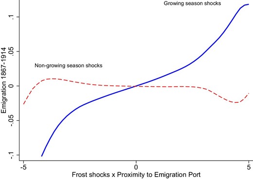
Non-parametric first stage relationship. Local means smooth. Bandwith: 2. The solid line displays the non-parametric relationship between the instrument and the log number of emigrants 1867–1914. The instrument is the interaction between the number of growing season frost shocks 1864–1867 and the proximity of the nearest emigration port. Proximity is defined as minus the log of distance. The dashed line displays the relationship between the placebo instrument, defined using non-growing season frost shocks, and the log number of emigrants 1867–1914. All variables have been residualized using the following covariates: county fixed effects, number of growing season frost shocks 1864–1867, proximity to the nearest emigration port, log population in 1865, log area, the arable share of land, log length of the growing season, latitude, longitude, proximity to the nearest town, nearest trade port, nearest railway, nearest weather station, and Stockholm, an urban indicator, an indicator for having at least one patent 1860–1864, log number of firms 1865, log power per output 1865, and a set of indicators for high soil quality for the production of barley, oats, wheat, dairy, and timber. Additionally, we include the interaction between growing season frost shocks 1864–1867 and proximity to the nearest town and trade port.
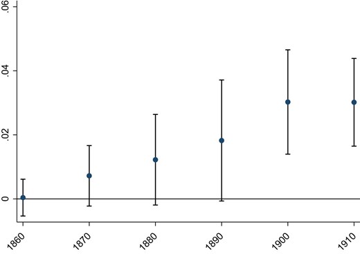
This figure displays OLS coefficients and 95% confidence intervals for the reduced-form effect of our instrument on the log number of patents in the 10-year period starting in the year denoted on the x-axis. The estimate for 1910 refers to the 1910–1914 period. The instrument is the interaction between the number of growing season frost shocks 1864–1867 and the proximity of the nearest emigration port. Proximity is defined as minus the log of distance. All regressions include county fixed effects, number of growing season frost shocks 1864–1867, proximity to the nearest emigration port, log population in 1865, log area, the arable share of land, log length of the growing season, latitude, longitude, proximity to the nearest town, nearest trade port, nearest railway, nearest weather station, and Stockholm, an urban indicator, an indicator for having at least one patent 1860–1864, log number of firms 1865, log power per output 1865, and a set of indicators for high soil quality for the production of barley, oats, wheat, dairy, and timber. Additionally, we include the interaction between growing season frost shocks 1864–1867 and proximity to the nearest town and trade port. Standard errors are clustered at the weather station level.
To get a sense of in which part of the economy that technological innovation appeared, we follow Nuvolari and Vasta (2015) and categorize patents into 14 different sectors. Figure 6 displays IV-estimates by patent sector.30 The first row shows that agricultural patents see one of the largest increases in innovation. This may reflect the fact that agriculture was characterized by labor-intensive production as well as being the largest sector of employment at the time. Indeed, Morell (2011) argues that most agricultural innovations at this time were labor-saving in nature. This is consistent with the fact that the agricultural lobby was one of the most politically vocal regarding the negative impact that emigration had on its availability of labor (Kälvemark 1972). In addition, food and machinery products see similarly large increases in innovation, while chemicals, construction, and transport categories see smaller, but also significant effects.
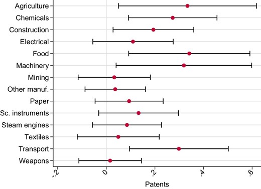
This figure displays the IV estimates of log emigration 1867–1914 on the log number of patents 1885–1914 by 14 different patent categories. The excluded instrument is the interaction between the number of growing season frost shocks 1864–1867 and the proximity to the nearest emigration port. Proximity is defined as minus the log of distance. All regressions include county fixed effects, number of growing season frost shocks 1864–1867, proximity to the nearest emigration port, log population in 1865, log area, the arable share of land, log length of the growing season, latitude, longitude, proximity to the nearest town, nearest trade port, nearest railway, nearest weather station, and Stockholm, an urban indicator, an indicator for having at least one patent 1860–1864, log number of firms 1865, log power per output 1865, and a set of indicators for high soil quality for the production of barley, oats, wheat, dairy, and timber. Additionally, we include the interaction between growing season frost shocks 1864–1867 and proximity to the nearest town and trade port. Standard errors are clustered at the weather station level. Bars indicate 95% confidence intervals.
5.1.1. Within-Municipality Analysis of Emigration Exposure and Innovation
Historical accounts suggest that a significant part of innovation in the late 19th century was labor-saving in nature (Fredholm 1879; Morell 2001). Yet, there is no straightforward way of categorizing the large number of patents in our data as labor saving or not. This section provides a more direct test of the relation between emigration and innovation by studying patent classes that were more or less exposed to emigration within the same municipality.31
Column (1) of Table 3 displays our main result—within municipalities, greater local exposure to emigration within a patent class is associated with more patenting in that class. The inclusion of both municipality and patent class fixed effects means that this result is net of all other types of emigration as well as certain sectors being more likely to have emigrants or innovation in general. The result in column (1) thus establishes a more direct link between emigration and innovation, indicating that differential emigration exposure even within a municipality matters for innovation. While this result is not causally identified, comparing estimates from Table 2 indicates that OLS estimates represent a lower bound of the effect of emigration on innovation in our setting. Assuming that this relationship holds within patent classes in a municipality, this indicates that the causal effect is positive.
Class-specific exposure to emigration within municipalities.
| Patents | |||||
|---|---|---|---|---|---|
| Dependent variable: | (1) | (2) | (3) | (4) | (5) |
| Municipal DPK-emigration | 0.002|$^{***}$| | 0.002|$^{***}$| | 0.002|$^{***}$| | 0.010|$^{***}$| | 0.006|$^{***}$| |
| (0.001) | (0.000) | (0.001) | (0.003) | (0.002) | |
| National DPK-emigration | 0.006|$^{***}$| | ||||
| (0.001) | |||||
| Total municipal emigration | 0.026|$^{***}$| | ||||
| (0.008) | |||||
| Patent class FE | Yes | No | No | Yes | Yes |
| Municipality FE | Yes | Yes | Yes | No | No |
| Municipality controls | No | No | No | Yes | Yes |
| Observations | 212,532 | 212,532 | 212,532 | 210,129 | 210,129 |
| Mean dependent variable | 0.023 | 0.023 | 0.023 | 0.023 | 0.023 |
Notes: OLS regressions. The dependent variable is the log number of patents 1885–1914 within a patent class in the German Patent Class System (DPK). Municipal DPK-emigration is the log municipal number of emigrants 1867–1914 with pre-emigration occupations related to the patent class. National DPK-emigration is the log national number of emigrants 1867–1914 related to the patent class. Total municipal emigration is the log municipal number of emigrants 1867–1914. All specifications control for log workers’ 1880 at the same level as the included emigration variables (1880 is the first available year in which we observe employment composition). Municipality controls include log area, the arable share of land, log length of the growing season, latitude, longitude, proximity to the nearest town, nearest trade port, nearest railway, nearest weather station, and Stockholm, an urban indicator, an indicator for having at least one patent 1860–1864, log number of firms 1865, log power per output 1865, and a set of indicators for high soil quality for the production of barley, oats, wheat, dairy, and timber. Standard errors are given in parentheses and are clustered at the municipality level. |$^{***}p<0.01$| .
By omitting patent-class fixed effects from the model, we can include national exposure to emigration by patent class. Column (2) shows that only dropping patent class fixed effects has little impact on the baseline estimate. In column (3), the estimate for national emigration is positive and three times larger than that for local emigration, which remains stable. Since many innovations likely had a national marke—both the product itself as well as the patent could be sold—this result suggests that innovators were also influenced by overall exposure to emigration when deciding to innovate. Finally, by dropping municipality fixed effects, we can estimate the effect of total municipal emigration on each patent class. Column (4) only drops the municipality fixed effect, showing that the estimate of local emigration grows substantially. When including both patent-class specific as well as total emigration in column (5), we see that both sources of emigration have positive and significant estimates, with the latter being approximately four times larger. While we cannot fully rule out that this may in part be due to measurement error, as total municipal emigration is measured more precisely, we interpret it as indicative of a spillover effect.
5.2. Capital and Labor Intensity
We next turn to the use of capital and labor in both the agricultural and industrial sector. If technology reduces the marginal productivity of labor, as in models of labor-saving technology (Zeira 1998; Acemoglu 2010), then we would expect production in emigration locations to increase their capital intensity and reduce their relative use of labor.
For agriculture, Table 4 displays results using data from 1910. We start by studying the effects of emigration on the share of unskilled agricultural workers per capita, as measured in the adult population of working age.32 These workers constituted the most mobile and landless workers, who could take on temporary jobs in the agricultural sector. Column (1) shows that emigration leads to a smaller share of such workers per capita, while column (2) shows that unskilled workers remain constant relative to the amount of arable land. To measure the use of capital in the agricultural sector, we use data on draft animals, namely horses and oxen. Draft animals may be seen as a direct measure of capital use in agriculture, but they are also linked to a variety of machines, such as threshers and mowers. Column (3) shows that the use of draft animals per area of arable land increases due to emigration. Since we specify both emigrants and the outcome variable in logarithms, we can interpret the coefficient as an elasticity of 0.08. In column (8) of Online Appendix Table B.5, we show that draft animals increased the most as measured relative to owned arable land rather than leased land. This is consistent with farm owners having easier access to credit, as they could use their land as collateral, allowing them to invest in draft animals and the associated new technologies (Hovde 1934).
Emigration and the agricultural sector.
| Workers per | Workers per | Draft animals per | Workers per | Workers per | Average | |
|---|---|---|---|---|---|---|
| capita | arable land | arable land | draft animal | horse | plotsize | |
| Dependent variable: | (1) | (2) | (3) | (4) | (5) | (6) |
| Emigrants 1867–1910 | −0.032|$^{***}$| | 0.014 | 0.079|$^{***}$| | −0.074|$^{**}$| | −0.111|$^{**}$| | |$-$|0.149 |
| (0.010) | (0.017) | (0.027) | (0.030) | (0.050) | (0.128) | |
| Region FE | Yes | Yes | Yes | Yes | Yes | Yes |
| Controls | Yes | Yes | Yes | Yes | Yes | Yes |
| Market access controls | Yes | Yes | Yes | Yes | Yes | Yes |
| Observations | 2,370 | 2,074 | 2,081 | 2,086 | 2,086 | 2,081 |
| F-statistic | 20.26 | 21.97 | 21.83 | 21.78 | 21.78 | 21.83 |
| Mean dependent variable | 0.05 | 0.04 | 0.15 | 0.23 | 0.29 | 2.91 |
Notes: 2SLS regressions. Workers per capita is the number of unskilled agricultural workers divided by the municipal population. Workers per arable land is the number of unskilled agricultural workers divided by arable land in hectares. Draft animals per arable land is the number of horses and oxen used in agriculture divided by arable land. Workers per draft animal is the number of unskilled agricultural workers divided by horses and oxen used in agriculture. Workers per horse is the number of unskilled agricultural workers divided by horses used in agriculture. Average plotsize is the average plotsize in hectares for agricultural plots. All outcome variables are measured in 1910. Emigrants 1867–1910 is the log number of emigrants 1867–1910. The excluded instrument is the interaction between the number of growing season frost shocks 1864–1867 and proximity to the nearest emigration port. Proximity is defined as minus the log of distance. All regressions include county fixed effects, the log population in 1865, as well as the number of growing season frost shocks 1864–1867 and the proximity to the nearest emigration port. Controls include log area, the arable share of land, log length of the growing season, latitude, longitude, proximity to the nearest town, nearest trade port, nearest railway, nearest weather station, and Stockholm, an urban indicator, an indicator for having at least one patent 1860–1864, log number of firms 1865, log power per output 1865, and a set of indicators for high soil quality for the production of barley, oats, wheat, dairy, and timber. Market Access controls include the interaction between growing season frost shocks 1864–1867 and proximity to the nearest town and trade port. The F-statistic refers to the Kleibergen–Paap F-statistic of the excluded instrument. Standard errors are given in parentheses and are clustered at the weather station level. |$^{**}p<0.05$|, |$^{***}p<0.01$|.
To more directly study the effect on the relative use of workers and capital, we estimate the effect on the number of unskilled agricultural workers relative to draft animals in column (4). The negative effect indicates that unskilled workers were reduced relative to draft animals, suggesting an increased capital intensity. In column (5), we show that this effect is driven by the substitution of workers for horses, rather than oxen.33 Interestingly, while both horses and oxen enabled the use of labor-saving technology, horses were a key component of the rationalization in agriculture at the time, as many of the new agricultural machines, such as mowing-machines, rakers, binders, and sowing-machines, were built for horsepower (Sjöström 1922; Morell 2001, 2011). Thus, this effect may not only reflect a change in production technique, but also indicate technology adoption, as the usage of horses is likely coupled with the usage of new technologies. Column (6) shows that there is a statistically insignificant negative effect on average plot sizes, indicating that emigration did not lead to land consolidation.
Turning to the industrial sector, we use data from the firm census in 1900 together with census data of the population in the same year. Table 5 displays our results. Similar to the case of agriculture, in column (1) we estimate the effect of emigration on manual industrial workers per capita. In contrast, however, we find a significant increase. Column (8) of Online Appendix Table B.8 explores to what extent the relative increase in the industrial sector is driven by stayers (shifting from agriculture) or by in-migrants, finding that both groups see an increase in the share of the working population devoted to the industrial sector throughout the 1890–1910 period.34 Together with the results in Table 4, this indicates that emigration caused structural change with workers leaving the agricultural sector for industry. Indeed, this is in line with historical evidence arguing that the more productive industrial sector could better afford the higher wages in emigration locations (see e.g. Schön 2000 and Ljungberg 1997).
Emigration and the industrial sector.
| Workers per | Power per | Power per | Equity per | Profits per | High-skill | |
|---|---|---|---|---|---|---|
| capita | output value | worker | worker | worker | ratio | |
| Dependent variable: | (1) | (2) | (3) | (4) | (5) | (6) |
| Emigrants 1867–1900 | 0.017|$^{**}$| | 0.009|$^{***}$| | 0.111 | 1.005|$^{*}$| | 0.521|$^{*}$| | 0.081|$^{**}$| |
| (0.009) | (0.003) | (0.159) | (0.532) | (0.305) | (0.039) | |
| Region FE | Yes | Yes | Yes | Yes | Yes | Yes |
| Controls | Yes | Yes | Yes | Yes | Yes | Yes |
| Market access controls | Yes | Yes | Yes | Yes | Yes | Yes |
| Observations | 2,376 | 2,388 | 2,388 | 2,375 | 2,328 | 2,376 |
| F-statistic | 14.54 | 14.01 | 14.01 | 14.54 | 15.57 | 14.54 |
| Mean dependent variable | 0.05 | 0.01 | 0.48 | 1.21 | 0.70 | 0.18 |
Notes: 2SLS regressions. Workers per capita is the number of manual non-agricultural workers divided by the municipal population in 1900. Power per output value is the amount of machine-generated horsepower divided by the output value in 1900. Power per worker is the amount of horsepower per manual industrial worker in the municipality in 1900. Equity per worker is average total equity of incorporated firms 1900–1919 divided by manual industrial workers in the municipality in 1900. Profits per worker is the average total profits of incorporated firms 1900–1919 divided by manual industrial workers in the municipality in 1900. High-skill ratio is the number of high-skilled industrial workers divided by all other industrial workers in the municipality 1900. Emigrants 1867–1900 is the log number of emigrants in 1867–1900. The excluded instrument is the interaction between the number of growing season frost shocks 1864–1867 and proximity to the nearest emigration port. Proximity is defined as minus the log of distance. All regressions include county fixed effects, the log population in 1865, as well as the number of growing season frost shocks 1864–1867 and the proximity to the nearest emigration port. Controls include log area, the arable share of land, log length of the growing season, latitude, longitude, proximity to the nearest town, nearest trade port, nearest railway, nearest weather station, and Stockholm, an urban indicator, an indicator for having at least one patent 1860–1864, log number of firms 1865, log power per output 1865, and a set of indicators for high soil quality for the production of barley, oats, wheat, dairy, and timber. Market Access controls include the interaction between growing season frost shocks 1864–1867 and proximity to the nearest town and trade port. The F-statistic refers to the Kleibergen–Paap F-statistic of the excluded instrument. Standard errors are given in parentheses and are clustered at the weather station level. |$^{*}p<0.1$|, |$^{**}p<0.05$|, |$^{***}p<0.01$|.
To measure the effect of emigration on the capital intensity of production, taking the scale of the sector into account, we construct a proxy for the capital share, namely machine power usage divided by output value. Column (2) shows that emigration leads to more power usage relative to output value, consistent with labor-saving technological change (Zeira 1998). Similarly, column (3) shows a positive effect of power usage relative to the number of manual industrial workers in the municipality, albeit with a statistically insignificant estimate. As an additional measure of capital intensity, we examine capital in the form of equity in incorporated firms 1900–1919. Incorporated firms were required to have a minimum level of capital in order to form, and capital could only be used to invest in assets that would stay in the firm, but not for running costs such as wages. Column (4) shows that average firm equity increased relative to the number of manual industrial workers in 1900, an indication of greater capital per worker. Thus, as column (1) showed an increase in industrial workers, the results in columns (2)–(4) also indicate a rising capital-labor ratio in the sector. While we cannot exclude that labor-augmenting technology increased in emigration municipalities, such as technology creating new tasks (Acemoglu and Restrepo 2019), the results indicate that the net effect of technological change in industry was labor-saving.
Column (5) of Table 5 documents an increase in firm profits per manual industrial worker, indicating that firms in high-emigration areas become more profitable in the long run. Lastly, in column (6), we use census data to estimate changes in the skill composition of the industrial workforce. Measured as the ratio of high-skilled employment to all other employment, we find a positive and significant effect. Thus, emigration appears to have favored skilled occupations relatively more in the industrial sector, typical for later stages of the industrial revolution (see e.g. Goldin and Katz 1998).
To give a more general picture of municipal economic effects, Figure 7 shows a binned scatterplot of the relationship between the instrument and municipal tax income in 1900. The instrument has a clear positive relationship with tax income over its full range. Column (8) of Online Appendix Table B.10 displays IV regression output, showing that the effect of emigration on tax income is positive and statistically significant. Emigration thus led to higher (taxable) incomes, indicating a positive effect on economic growth in the long run.
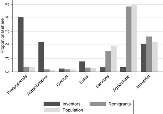
Occupational distribution among inventors, migrants, and in the population. This figure displays the share of each occupational sector among return migrants and inventors 1875–1914 alongside population shares 1880–1910. Occupational sectors follow the seven major groups of the Historical International Standard Classification of Occupations (HISCO). Professionals includes professional, technical, and related workers. Administrative includes administrative and managerial workers. Clerical includes clerical and related workers. Sales includes sales workers. Service includes service workers. Agricultural includes agricultural, animal husbandry, forestry workers, fishermen, and hunters. Industrial includes production and related workers, transport equipment operators, and laborers.
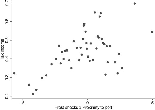
This figure displays a binned scatter plot for the relationship between the instrument and municipal tax income in 1900. The instrument is the interaction between the number of growing season frost shocks 1864–1867 and the proximity of the nearest emigration port. Proximity is defined as minus the log of distance. Both tax income and the instrument have been residualized using the following covariates: county fixed effects, number of growing season frost shocks 1864–1867, proximity to the nearest emigration port, log population in 1865, log area, the arable share of land, log length of the growing season, latitude, longitude, proximity to the nearest town, nearest trade port, nearest railway, nearest weather station, and Stockholm, an urban indicator, an indicator for having at least one patent 1860–1864, log number of firms 1865, log power per output 1865, and a set of indicators for high soil quality for the production of barley, oats, wheat, dairy, and timber. Additionally, we include the interaction between growing season frost shocks 1864–1867 and proximity to the nearest town and trade port.
5.2.1. Wages
Wages could rise with emigration for at least two reasons. First, and most directly, emigration may increase wages by reducing the supply of labor. Second, workers may more credibly threaten to emigrate when they have migrant networks overseas, strengthening their bargaining power and, hence, wages. Consistent with this, Karadja and Prawitz (2019) show that the Swedish labor movement advanced in communities with relatively more emigration.35 Apart from its likely positive effect on wages, the presence of labor unions may increase labor costs in other dimensions, such as working hour restrictions and safety requirements.
While we lack data on wages at the municipal level, we employ yearly data on agricultural wages at the county level from Jörberg (1972b). This is the only consistent wage series for the second part of the 19th century. It covers wages for landless agricultural day laborers who do mainly unskilled work. Scattered across Sweden, these types of workers made up about half of the agricultural working class (Jungenfelt 1959), and their employment terms resembled those of industrial and construction workers (Enflo, Lundh, and Prado 2014). The official series is representative of the whole county, including towns, cities, and rural areas, and it is considered that it reflects the level of day wages of other unskilled trades as well (Ljungberg 1997), suggesting that it is a good proxy for low-skilled wages more in general.36
We focus on long-term changes at the county level, running OLS regressions of cumulative emigration on wage growth, defined as the wage rate between 1860 and 1914.37 As before, we define emigration as the natural logarithm of the number of emigrants and include the natural logarithm of the population at the baseline to scale emigration to per capita levels. Additionally, we include the natural logarithm of the county area, the share of urban municipalities, and the arable share of land as controls. The results are displayed in Table 6. Although we only have 23 observations,38 there is a strong positive relationship between emigration and long-term wage growth. The coefficients indicate that a 10% increase in emigration is associated with an increase of roughly 5–7 percentage points in the nominal wage rate (columns 1 and 2) and a 7–11 percentage point increase in the real wage rate (columns 3 and 4).
Emigration and low-skilled wage growth.
| Nominal wage growth | Real wage growth | |||
|---|---|---|---|---|
| Dependent variable: | (1) | (2) | (3) | (4) |
| Emigrants 1867–1914 | 0.516|$^{**}$| | 0.717|$^{***}$| | 0.684|$^{**}$| | 1.079|$^{***}$| |
| (0.203) | (0.221) | (0.271) | (0.296) | |
| Controls | No | Yes | No | Yes |
| Observations | 23 | 23 | 23 | 23 |
| Mean dependent variable | 2.66 | 2.66 | 3.62 | 3.62 |
Notes: OLS regressions. The dependent variable is wage growth for day laborers in agriculture between 1860 and 1914. Emigrants 1867–1914 is the log number of emigrants from 1867 until 1914. All regressions include log population in 1865. Controls include log area, the share of urban municipalities, and the arable share of land. Robust standard errors are reported in parentheses. |$^{**}p<0.05$|, |$^{***}p<0.01$|.
5.3. Return Flows from the United States
Emigration may influence innovation in origin communities through information and capital flows sent back home. To examine this possibility, we start by considering if return migrants contribute to our innovation results by obtaining the patent rights themselves, perhaps for new ideas accumulated abroad. While almost a fifth of the emigrants eventually returned to Sweden, many of these returned after the start of World War I, when our sample period ends. Fewer than 10% had returned in 1910.39 Moreover, we detect significant effects on innovation as early as the 1880s, as seen in Online Appendix Figure B.3. Nevertheless, these return migrants could have been influential. Figure 8 displays the occupational distribution of return migrants, inventors, and the full population following the Historical International Standard Classification of Occupations (HISCO) (see Van Leeuwen, Maas, and Miles 2002). Returnees were chiefly within the agricultural sector, followed by the service and industrial sectors. By contrast, the inventors in our data were mostly high skilled. The clearly most common profession of inventors is engineer with about 30% of the patents, with the second most common being managers with about 10%. No other profession exceeds 5% of the share of patents.
Emigration and patents weighted by return flow measures.
| Return flow weighted patents | ||||||||||
|---|---|---|---|---|---|---|---|---|---|---|
| Returnee occupations | US style patents | |||||||||
| OLS | IV | OLS | IV | |||||||
| Dependent variable: | (1) | (2) | (3) | (4) | (5) | (6) | (7) | (8) | (9) | (10) |
| Emigrants 1867–1914 | −0.610|$^{**}$| | −0.494|$^{***}$| | −1.997|$^{**}$| | −1.508|$^{**}$| | −1.613|$^{**}$| | −0.006|$^{**}$| | −0.005 | −0.039|$^{*}$| | −0.043|$^{*}$| | −0.046|$^{**}$| |
| (0.227) | (0.176) | (0.884) | (0.710) | (0.641) | (0.003) | (0.003) | (0.021) | (0.022) | (0.021) | |
| Region FE | Yes | Yes | Yes | Yes | Yes | Yes | Yes | Yes | Yes | Yes |
| Controls | No | Yes | No | Yes | Yes | No | Yes | No | Yes | Yes |
| Market access controls | No | No | No | No | Yes | No | No | No | No | Yes |
| Observations | 2,376 | 2,376 | 2,376 | 2,376 | 2,376 | 2,376 | 2,376 | 23,76 | 2,376 | 2,376 |
| F-statistic | 16.76 | 20.36 | 21.01 | 16.76 | 20.36 | 21.01 | ||||
| Mean dependent variable | |$-$|0.64 | |$-$|0.64 | |$-$|0.64 | |$-$|0.64 | |$-$|0.64 | |$-$|0.02 | |$-$|0.02 | |$-$|0.02 | |$-$|0.02 | |$-$|0.02 |
Notes: OLS and 2SLS regressions. The dependent variable is a weighted measure of patents 1885–1914 per 1000 inhabitants. Patents in columns (1)–(5) are weighted more highly if the inventor has an occupation that is more typical for return migrants than for the general population. Patents in columns (6)–(10) are weighted more highly if they belong to patent classes that are more typical in the United States than in Sweden. Emigrants is the log number of emigrants in 1867–1914. The excluded instrument is the interaction between the number of growing season frost shocks 1864–1867 and proximity to the nearest emigration port. Proximity is defined as minus the log of distance. All regressions include county fixed effects, the log population in 1865, as well as the number of growing season frost shocks 1864–1867 and the proximity to the nearest emigration port. Controls include log area, the arable share of land, log length of the growing season, latitude, longitude, proximity to the nearest town, nearest trade port, nearest railway, nearest weather station, and Stockholm, an urban indicator, an indicator for having at least one patent 1860–1864, log number of firms 1865, log power per output 1865, and a set of indicators for high soil quality for the production of barley, oats, wheat, dairy, and timber. Market Access controls include the interaction between growing season frost shocks 1864–1867 and proximity to the nearest town and trade port. The F-statistic refers to the Kleibergen–Paap F-statistic of the excluded instrument. Standard errors are given in parentheses and are clustered at the weather station level. |$^{*}p<0.1$|, |$^{**}p<0.05$|, |$^{***}p<0.01$|.
Yet, return migrants may influence innovation at home indirectly by spreading new knowledge, and migrants still abroad may transmit information via mail correspondence. Alternatively, a small group of high-skilled inventors may have been instrumental in the technological upswing. To test for these possibilities, we measure the extent to which a Swedish patent belongs to a patent class that is more common in the United States than in Sweden. Using aggregate information on the distribution of patent classes in 1900 in both Sweden and the United States, we then create a new weighted patent measure at the municipality level, similar to the return-migration patent measure described above. In particular, for each patent in a technology class, we calculate the difference between the share of US patents and the share of Swedish patents within that technology class.40 Thus, we give greater weight to patents in patent classes that are relatively more common in the United States than in Sweden. For example, if patent class A makes up 90% of US patents and 50% of Swedish patents, we assign patents in class A a value of |$0.4=0.9-0.5$|. Results are presented in columns (6)–(10) of Table 7. Similar to the case with return migrant occupations, we find that high-emigration municipalities become less likely to patent in areas that are relatively more common in the United States than in Sweden.41
Economic remittances may also have played a role if migrants provided capital for investments back home. There is, unfortunately, no source of data that allows an analysis of the spatial distribution of remittances by region in Sweden. Nevertheless, we note that in terms of aggregate flows, the ratio of remittances to GDP was smaller for Sweden as compared to Ireland and “almost insignificant” relative to Italy (Babcock 1914).
Ultimately, in our historical context, where remittances were limited and the only transatlantic communication method was by regular mail, the most comprehensive way of assessing the importance of return flows is perhaps by studying the return migration in general. Here, it is important to note that for return migration to explain our results it is necessary that return migrants positively affected technological change in the same municipalities that exhibited high emigration. However, using our IV identification strategy it is difficult to separate emigration from return migration, as municipalities with high emigration also may have relatively more return migrants. Therefore, to study the association between emigration, return migration and technological change, we estimate OLS regressions displayed in Table 8. Column (1) shows the positive relationship between emigration and patents 1867–1914, controlling for our baseline covariates and county fixed effects. Return migration has a smaller but similarly positive and significant correlation with patents shown in column (2). However, once we include both emigration and return migration in column (3), the correlation with return migration effectively disappears. The point estimate is reduced from 0.080 to 0.006 and is no longer statistically significant. By contrast, the estimate for emigration is unaffected and remains strongly significant. Repeating this analysis for fee-weighted patents in columns (4)–(6), we find the same pattern. Column (8) of Online Appendix Table B.9 provides the same tests for our agricultural and industrial outcomes. Overall, results show a small and often insignificant coefficient on return migration once controlling for emigration, which by itself has a larger and mostly significant estimate.
Emigration, return migration, and patents.
| Patents | Patent fees | |||||
|---|---|---|---|---|---|---|
| Dependent variable: | (1) | (2) | (3) | (4) | (5) | (6) |
| Emigrants | 0.262|$^{***}$| | 0.259|$^{***}$| | 0.368|$^{***}$| | |||
| (0.040) | (0.039) | (0.057) | ||||
| Return migrants | 0.080|$^{***}$| | 0.006 | 0.096|$^{**}$| | 0.096|$^{**}$| | |$-$|0.010 | |
| (0.025) | (0.018) | (0.035) | (0.035) | (0.028) | ||
| Region FE | Yes | Yes | Yes | Yes | Yes | Yes |
| Controls | Yes | Yes | Yes | Yes | Yes | Yes |
| Observations | 2,388 | 2,388 | 2,388 | 2,388 | 2,388 | 2,388 |
| Mean dependent variable | ||||||
| y-mean | 0.62 | 0.62 | 0.62 | 0.99 | 0.99 | 0.99 |
Notes: OLS regressions. All regressions include county fixed effects, the log population in 1865, as well as proximity to the nearest emigration port. Controls include log area, the arable share of land, log length of the growing season, latitude, longitude, proximity to the nearest town, nearest trade port, nearest railway, nearest weather station, and Stockholm, an urban indicator, an indicator for having at least one patent 1860–1864, log number of firms 1865, log power per output 1865, and a set of indicators for high soil quality for the production of barley, oats, wheat, dairy, and timber. Robust standard errors are given in parentheses. |$^{**}p<0.05$|, |$^{***}p<0.01$|.
Together, our results indicate that return flows from the United States did not play a major role in explaining the effects we find on technological change. Instead, it appears more likely that local economic incentives changed as labor became more scarce and costly. Nevertheless, we cannot exclude that return migrants contributed to innovation in the aggregate.
5.4. Robustness and Placebo Tests
In Online Appendix A, we provide detailed descriptions of several robustness and placebo tests. Here, we summarize the results briefly. First, we use non-growing season shocks as well as proximities to non-emigration ports and towns in order to create placebo instruments, finding that they do not affect any of our outcomes. Results are also robust to assuming violations of the exclusion restriction following Conley, Hansen, and Rossi (2012).
Next, we show that results are robust to various functional forms for innovation in addition to our baseline log(patents+1), including expressing patents per capita, per engineer, using the inverse hyperbolic sine transformation, as well as using count data models. Results are also robust to dropping random subsets of counties, controlling for various non-linear functions of port proximity, frost shocks, latitude, and longitude, varying the level of spatial fixed effects, as well as different methods of computing standard errors.
Column (8) of Online Appendix A.3 concludes with a discussion of potential measurement error in emigration and the differences in estimates between OLS and IV specifications.
6. Discussion and Conclusion
This paper explores the effects of mass migration on technological change in sending communities by studying one of the largest migration episodes in history; during the Age of Mass Migration, 30 million Europeans left their home countries to settle in the United States. We focus on Sweden, where about a quarter of the initial population migrated.
Our main result is that emigration caused an increase in innovation in the origin locations, as measured by both the number and the economic value of patents. Using an instrument based on travel costs and the severe weather shocks that sparked the initial wave of migration to the United States, our IV estimates suggest that a 10% increase in the number of migrants during the main Swedish transatlantic migration period 1867–1914 would have increased the number of patents by about 6%. In addition, we show that emigration is not only positively related to the invention of new ideas, but also to an increased capital intensity in production. In general, our estimates indicate substitution from labor to capital in both the agricultural and industrial sectors at the turn of the century.
Together, our results are consistent with the induced innovation hypothesis, that is, emigration leading to higher labor costs, encouraging investments in labor-saving technologies. Several pieces of evidence support this conclusion. For example, the finding of a link between emigration and innovation within patent classes in a municipality, the reduction in workers per draft animal in agriculture, and the greater use of machine power relative to output value in the industrial sector. We find less support for alternative channels connected to return flows from the United States, such as human capital accumulation abroad. Nevertheless, we recognize that other forces may have been at play that are outside of the scope of this investigation.
This paper is closely related to our companion paper Karadja and Prawitz (2019), which finds a positive effect of emigration on labor organization. As noted also by Schön (2000), it is likely that these unions contributed to high labor costs, either directly by pushing up wages or indirectly by demanding better working conditions. Both may have affected labor-saving technology (cf. Alesina, Battisti, and Zeira 2018).
A few features of our empirical context may be important to note in order to put our findings into perspective. The relatively high and widespread human capital in Sweden, due to the introduction of universal basic education in 1842, may have been an important precondition. Moreover, given the abundance of low-wage labor and labor-intensive production processes at the onset of its migration episode, the scope for technological change may have been particularly high once emigration changed labor market conditions. Indeed, Swedish economic historians as well as contemporary observers characterize the technology of the period as largely labor-saving, echoing scholars studying similar periods of modernization in other places (see e.g. Landes 1969; Habakkuk 1962; Allen 2009). To what extent the relationship between emigration and technology is similar in modern economies is an open question.
Acknowledgements
The editor in charge of this paper was Imran Rasul.
Acknowledgements: We thank Torsten Persson, David Strömberg, Jakob Svensson, Philippe Aghion, Konrad Burchardi, Davide Cantoni, Jon de Quidt, Nathan Lane, Andreas Madestam, Peter Nilsson, Nathan Nunn, Maria Petrova, and Per Pettersson-Lidbom, as well as numerous seminar and conference participants for helpful comments. We acknowledge funding from the Jan Wallanders och Tom Hedelius stiftelse samt Tore Browaldhs stiftelse and the Marianne and Marcus Wallenberg Foundation.
Footnotes
The identification strategy is based on Karadja and Prawitz (2019).
Crucially, by only using the interaction between frost shocks and emigration port proximity as our instrument, we are able to control for the direct effects that these two variables may have by themselves.
While we lack data on wages in the industrial sector, economic historians argue that our used wage series is a reasonable proxy for unskilled wages in other sectors as well (Ljungberg 1997).
In terms of immigration and innovation during this period, Sequeira, Nunn, and Qian (2020) find (among other results) that immigration positively affected patents in the United States.
O’Rourke and Williamson (1995) find that the transatlantic emigration increased low-skilled wages by about 12% in both the agricultural and the urban sector between 1870 and 1910. Ljungberg (1997) argues that emigration accounted for at least one-third of the increase in low-skilled wages in agriculture.
In real prices, the cost of applying and renewing a patent for the maximum number of 15 years was similar to today’s cost of keeping a patent in force for the same duration.
The compilation and digitization process of the patent data is described in Online Appendix C.1.
In Online Appendix Table A.7, we show that our results are robust to counting patents by splitting each patent into equal shares for all the inventors of a patent.
The industrial data were graciously shared by Olof Ejermo and Mats Olsson. See http://www.historicalmanufacturingcensus.se.
More precisely, they refer to the periods 1901–1905, 1907–1911, and 1915–1919. Data are collected in 1906, 1912, and 1920.
We obtained the data from the Swedish Migration Center in Karlstad, Sweden.
As we lack digitized data from the church books after 1895, all later migrants are obtained from the passenger lists. Before 1895, the parish data reported more migrants than the shipping line data for about 50% of our municipal-year observations, while the latter reported more migrants for about 25%.
The median and mean distance from our municipality centroids are 36 and 39 kilometers, respectively.
Using Swedish county-level data from 1860 to 1880, Karadja and Prawitz (2019) show empirically that frost significantly predicts worse harvest outcomes.
We define proximity as minus the log of distance to the municipality centroid.
As there are a considerable amount of municipalities without any patents, we add one to the number of patents before taking the natural logarithm. In Online Appendix A, we show that our outcomes are robust to using the inverse hyperbolic sine function instead of the natural logarithm, defining patents in per capita terms, as well as using count data models.
All continuous variables are de-meaned to facilitate the interpretation, including the number of frost shocks and the proximity to an emigration port.
There are 24 historical counties. In Online Appendix A, we show that our results are robust when using only three regional fixed effects for the major lands of Sweden as well as when excluding fixed effects entirely.
The standard deviation of our instrument is 2.14.
Online Appendix Table A.8 shows that results are similar if we restrict emigration to 1867–1900, the bulk of the emigration episode, and study its effect on patents from 1900 to 1914.
Indeed, in our data, firms were less likely to sell patent rights as compared to independent patentees. In Online Appendix Table B.2, we also show that emigration affected both transferred and never-transferred patents.
Since we only have data on patent fees starting in 1885, we studied the effect on fee-weighted patents 1885–1914.
As an alternative measure of patent quality, we make use of USPTO patent data on all patents granted in the United States 1867–1914 with an individual located in Sweden. While these are relatively few, only about 8% of municipalities are involved in a USPTO patent. This allows us to also weight patents by citations. The results are presented in Online Appendix Table B.3, where we show that emigration positively affected USPTO patents.
This gradual increase also indicates that the effect of emigration on patents is not driven by the patent law reform of 1885. Online Appendix Figure B.3 shows that there are statistically significant effects for individual years prior to 1885. Column (8) of Online Appendix Table A.9 also displays the effect of emigration 1867–1885 on patents in the same period finding positive, but statistically insignificant estimates for the period as a whole.
Since we only have data on DPK class starting in 1885, we study the effect on patents 1885–1914.
We do so by matching emigrants to patent classes using data on their pre-emigration occupations. A detailed description of this matching procedure is provided in column (8) of Online Appendix Table C.3. Repeating this procedure for the 89 classes in the German Patent Class System (DPK), the resulting data set has a maximum of |$89\times 2,388$| observations. Column (8) of Online Appendix Table A.23 shows the results when aggregating patents into 12 sectors instead of using the finer DPK classification with 89 groups.
We define unskilled workers following the Historical International Standard Classification of Occupations (HISCO) (see Van Leeuwen, Maas, and Miles 2002).
The effect on workers per oxen is shown in column (8) of Online Appendix Table B.6.
We make use of linked census data from Eriksson (2015) to define inhabitants as stayers or in-migrants.
See also Schön (2000), arguing that social and political changes in this period spurred wage growth by improving workers’ power.
There is considerable variation in wages across counties, suggesting that local markets were not fully connected, with the coefficient of variation being about 0.25 in 1900.
Online Appendix Figure B.4 depicts the national annual wage growth in this series. The mean wage growth was about 3% during 1860–1914.
Since one county, Blekinge, failed to report its wages, we lack one county.
The US patent distribution by NBER technology class is from the USPTO Historical Patent Data Files.
Column (8) of Online Appendix Table B.4 shows that the results are robust to construct our outcome variable as the relative technological proximity between the United States and Sweden using Jaffe’s (1986)) metric. In particular, we compute the uncentered correlation between a municipality’s share of patents in each NBER technology class and the corresponding national shares: |$\rho _{i, N} = P_i P^{\prime }_N/\big[(P_i P^{\prime }_i) (P_N P^{\prime }_N)\big]^{1/2}$|, where |$P_k$| is a vector of shares of patents of each class at the national level |$k=N$| (United States or Sweden) or for a municipality |$k=i$|. To construct the relative proximity to the United States, we finally compute the difference between |$\rho _{i, \text{US}}$| and |$\rho _{i, \text{Sweden}}$|.
