


Abstract
Morphology, habitat and various selective pressures (e.g. social and sexual selection) can influence the evolution of acoustic signals, but the relative importance of their effects is not well understood. The order Psittaciformes (parrots, sensu lato) is a large clade of very vocal and often gregarious species for which large‐scale comparative studies of vocalizations are lacking. We measured acoustic traits (duration, sound frequency, frequency bandwidth and sound entropy) of the predominant call type for >200 parrot species to test: (1) for associations with body size; (2) the acoustic adaptation hypothesis (AAH) (predicting differences between forest and open‐habitat species); (3) the social complexity hypothesis (predicting more complex calls in gregarious species) and (4) influences of sexual selection (predicting correlated evolution with colour ornamentation). Larger species had on average longer calls, lower sound frequency and wider frequency bandwidth. These associations with body size are all predicted by physical principles of sound production. We found no evidence for the acoustic adaptation and social complexity hypotheses, but perhaps social complexity is associated with vocal traits not studied here, such as call repertoire sizes. More sexually dichromatic species had on average simpler calls (shorter, with lower entropy and narrower frequency bandwidth) indicating an influence of sexual selection, namely an evolutionary negative correlation between colour ornamentation and elaborate acoustic signals, as predicted by the transference hypothesis. Our study is the first large‐scale attempt at understanding acoustic diversity across the Psittaciformes, and indicates that body size and sexual selection influenced the evolution of species differences in vocal signals.
Abstract

INTRODUCTION
The evolution of acoustic signals can be influenced by morphological differences among species (Bradbury & Vehrencamp, 2011), by the type of habitats in which different species live and communicate (Brumm & Naguib, 2009; Ey & Fischer, 2009), and by the social or sexual functions of those signals. Many comparative studies, on several different taxa (e.g. insects: Couldridge & Van Staaden, 2004; anurans: Bosch & De la Riva, 2004; Kime et al., 2000; Zimmerman, 1983; mammals: Brown et al., 1995; García‐Navas & Blumstein, 2016; Luo et al., 2017; Mitani & Stuht, 1998; Peters & Peters, 2010; birds: Boncoraglio & Saino, 2007; Gomes et al., 2017; Ligon et al., 2018; Wallschläger, 1980), have shown that acoustic signals evolve influenced by one or some of these factors. Nonetheless, we have limited information on the relative importance of these several influences (morphology, habitat, social and sexual functions) on the evolution of species differences in acoustic signals. To our knowledge, no comparative work has simultaneously tested the effects of morphology, habitat and proxies for social and sexual selection as predictors in the same statistical models, to evaluate and compare their influences on acoustic signals.
Body size is perhaps the best understood predictor of among‐species differences in acoustic signals. Larger species generally use lower sound frequencies (e.g. birds: Wallschläger, 1980; crickets: Moradian & Walker, 2008; anurans: Gingras et al., 2013), particularly lower minimum frequencies (Friis, Sabino, et al., 2021; Martin et al., 2017), because large vocal organs and tracts are required to produce and broadcast low frequencies efficiently (Bradbury & Vehrencamp, 2011; Fletcher, 2004). Among passerine birds, larger species were also found to have longer songs (Badyaev & Leaf, 1997; Price & Lanyon, 2004) and vocalize or sing with higher sound amplitudes (Calder, 1990; Cardoso, 2010; Jurisevic & Sanderson, 1998), likely because of their larger air‐sacs and strength of respiratory muscles (Suthers, 1999).
Habitat type is another well‐known influence on the evolution of acoustic signals. As per the acoustic adaptation hypothesis (hereafter AAH; Hansen, 1979; Morton, 1975; Wiley & Richards, 1978), forested habitats are predicted to select for signals with lower sound frequency, less frequency modulation and longer durations of elements and of intervals, compared to open habitats. This is because the transmission of higher frequencies is more strongly dampened by foliage and other vegetation, and vegetation‐induced sound degradation blurs fast frequency or time modulations (Blumenrath & Dabelsteen, 2004; Graham et al., 2017). The AAH has been tested and found support in different vertebrate groups, albeit with effect sizes that are generally small and variable across taxa (reviewed in Boncoraglio & Saino, 2007; Ey & Fischer, 2009).
Species differences in acoustic signals can also arise from selection related to their social and sexual functions. The social complexity hypothesis predicts greater complexity in the signalling system of gregarious species, as opposed to solitary or pair‐living species, because of the need to convey a greater diversity of messages and/or to distinguish among a larger number of individuals in a group (Freeberg, 2006; Freeberg et al., 2012). This prediction of higher signal complexity in social species has gained empirical support from studies in several vertebrate and non‐vertebrate taxa, including for the specific case of acoustic signals (reviewed in Peckre et al., 2019). Acoustic signals can also have sexual functions, such as attracting mates or repelling same‐sex competitors, and sexual selection may thus strongly influence them, for example causing the evolution of elaborate signals such as bird songs (Gil & Gahr, 2002). Although sexual selection often explains the evolution of complex acoustic signals, such as long or diverse bird songs (Byers & Kroodsma, 2009; Robinson & Creanza, 2019; Soma & Garamszegi, 2011), it can lead to different and even opposed phenotypic outcomes. For example, it was suggested that strong sexual selection for one type of signal (e.g. ornamentation or visual signals) could be associated with reduced selection for, and therefore reduced elaboration in, other signals (e.g. acoustic), which would on average result in a negative correlation between the elaboration of different types of signals. This idea was first suggested by Darwin (1871) and later elaborated and coined as the transference hypothesis (Gilliard, 1956; Johnson, 1999; Schluter & Price, 1993).
Comparative work on acoustic signals has focused primarily on certain taxa and types of vocalizations, notably, among birds, on Passerine songs. Other taxa and other types of vocalizations are less studied. This is the case for the Psittaciformes (parrots and allies, hereafter parrots), an avian order well known for being highly vocal (de Araújo et al., 2011; Fernández‐Juricic & Martella, 2000), showing vocal learning (Bradbury & Balsby, 2016; Illes et al., 2006; Montes‐Medina et al., 2016) and with many species that live gregariously and rely on acoustic communication to mediate complex social interactions (de Araújo et al., 2011; Forshaw, 2010). These characteristics make parrots a promising group to investigate different influences on the evolution of acoustic signals, but very little comparative work on their calls was yet attempted (Medina‐García et al., 2015). Here we used a citizen‐science repository of acoustic recordings (Xeno‐canto; www.xeno‐canto.org) to measure acoustic traits (call duration, dominant frequency, frequency bandwidth and sound entropy) of the most common call type in 252 parrot species worldwide. We then used this novel dataset of acoustic recordings to teste for:
Scaling with body size, with smaller species predicted to use high dominant frequency, narrow frequency bandwidth and shorter calls.
Associations between acoustic traits and habitat type, with forest species predicted by the AAH to use lower frequencies and longer calls than open‐habitat species.
Associations with gregariousness, with gregarious species predicted by the social complexity hypothesis to have more complex calls (i.e. longer calls, with wider frequency bandwidth and/or higher sound entropy) than solitary or pair‐living species.
Associations with colour ornamentation, as sexual selection may cause either positively correlated evolution between sexual ornaments and call complexity or, as per the transference hypothesis, negatively correlated evolution.
By testing these different predictions, we aim at comparing the importance of morphological, environmental and functional influences for the evolution of acoustic differences among species.
MATERIALS AND METHODS
Acoustic recordings and measurements
For each species of Psittaciformes with recordings available in the Xeno ‐ Can to online repository (www.xeno‐canto.org; accessed in November 2019), we downloaded 1–5 recordings per species, depending on availability and sound quality (mean 2.6 ± 1.1 SD). We studied how parrot species most commonly sound like, because this should be how animals most often detect their conspecifics at long distances or when out of sight. For this we selected recordings containing the commonest call types of each species, as described in the Handbook of the Birds of the World Alive (hereafter HBW; del Hoyo et al., 2018), and that had good sound quality with little background or overlapping noise. We selected 1–5 adult calls per recording (mean 4.7 ± 0.8 SD) that were described in HBW as the commonest call types for that species. Here, call type refers to acoustically distinct calls. When the HBW did not describe the commonest calls of a species, we selected the most represented calls in Xeno‐Canto. We a nalysed 662 recordings from 252 species (64% of all Psittaciformes species), including 235 species in the family Psittacidae, 16 in Cacatuidae and one in Strigopidae.
We converted sound files (originally in mp3 format) to wave format with a sampling rate of 44 kHz using the warbleR package (Araya‐Salas & Smith‐Vidaurre, 2017) in R 4.1.1 (R Core Team, 2021). Mp3 compression does not cause measurement bias but may reduce precision of individual sound frequency measurements, although by a small degree compared to the large differences in sound frequency across species (Araya‐Salas et al., 2019). We further increased precision by averaging measurements across several calls (up to five) per recording, and several recordings per species.
We measured acoustic traits of calls using the software Avisoft‐SasLab Pro (Avisoft, Specht, 2004). First, in the spectrogram view of Avisoft (spectrogram settings: FFT length 512, flat top window, and 87.5% window overlap, which correspond to a resolution of 2.9 ms and 43 Hz; Figure 1), we marked the beginning and end times of each call for measurement, up to five calls per recording depending on availability and sound quality. For recordings with more than one call type described in the HBW as common calls, we measured up to three calls of the type most represented in the recording, and up to two of the other types in the recording that are also described as common in HBW. This procedure should provide a better approximation to how the species commonly sounds like compared to, somewhat arbitrarily, measuring only one of the call types. For species whose calls were described in HBW as containing multiple or repeated sound elements, typically very tightly together, we considered sound elements separated by intervals smaller than 100 ms as part of the same individual call. For species whose calls were not described as normally containing multiple elements, we used a longer time interval, 300 ms, as the threshold to consider multiple elements as part of the same call. In both cases, these thresholds agreed with our intuitive perception of call delimitation, based on hearing the full call bouts in the recordings.
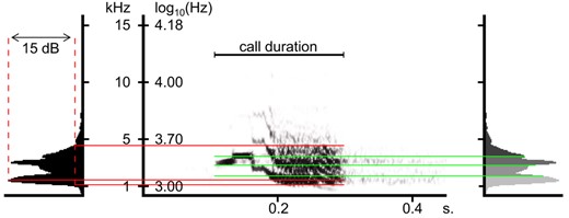
Spectrogram of a Kawall's amazon (Amazona kawalli) call, illustrating some of the acoustic measurements. Red lines towards the power spectrum on the left illustrate peak frequency (that with highest cumulative sound amplitude across the call), and maximum and minimum frequencies (those at which amplitude falls 15 dB below that of the peak frequency). Green lines towards the power spectrum on the right illustrate frequency quartiles: i.e. the three frequencies that separate the four sound energy quartiles. Spectrogram settings as described in the methods, except that here the spectrogram was trimmed at 15 kHz for ease of viewing
We measured four acoustic traits of each call: duration (from the marked start and end times of the call), dominant frequency, frequency bandwidth and sound entropy using automated measurement tools in Avisoft. Dominant frequency and frequency bandwidth were measured in two alternative manners. First, we measured peak frequency (i.e. the frequency with highest cumulative sound amplitude in the power spectrum of the call) and measured frequency bandwidth as maximum minus minimum frequencies, defining maximum and minimum frequencies as those at which cumulative amplitude falls −15 dB below that of the peak frequency (hereafter MaxMin bandwidth). We chose a threshold of −15 dB because it captured the vast majority of sound energy in calls (Figure 1), although being resilient to interfering noise in most recordings. Using larger amplitude thresholds could cause dismissing recordings of little recorded species, because of noise interference with the automated measurements. The second approach was assessing dominant frequency as the 50th energy percentile in the power spectrum and assessing frequency bandwidth as the inter‐quartile frequency difference (i.e. the differences between the 75th and the 25th energy percentiles). Inter‐quartile bandwidth focuses on the frequency interval containing most of the sound energy in the songs, whereas MaxMin bandwidth encompasses a broader range of frequencies in the calls. Finally, as an indication of harmonic complexity, we measured sound entropy, computed as the spectral Wiener entropy (the geometric mean of the spectrum divided by its arithmetic mean; Specht, 2004), which is lowest for pure and simple harmonic sounds, and augments as the amount of harmonic deviations increase. All raw frequency measurements (i.e. before bandwidth differences were computed, or any averaging was made) were taken in log10 Hz, as a logarithmic, ratio scale of sound frequency best agrees with how animals perceive and modulate sound frequency (Cardoso, 2013). We also log10‐transformed the duration of calls (log10 seconds) to correct its right‐skewed distribution.
To test the within‐species reliability of our measurements, across different recordings, we first averaged acoustic measurements per recording, so that each recording is used as one statistical unit. We then computed repeatability running a linear mixed effect model for each acoustic trait and using species as random factor (Nakagawa & Schielzeth, 2010) with the package rptR (Stoffel et al., 2017). Within‐species repeatability across recordings was high (>0.5) for peak frequency (R = 0.85), 50th frequency percentile (R = 0.82), MaxMin bandwidth (R = 0.59) and inter‐quartile bandwidth (0.65) and entropy (R = 0.56), and lower, but still highly significant, for call duration (R = 0.336; in all cases p < 0.001). The high within‐species repeatability of most measurements indicates that our measurements reliably characterize acoustic differences among species. The lower repeatability for call duration may be because calls can be terminated at different points or contain a variable number of element repetitions, and indicates that results of analyses on call duration should be conservative. As we measured dominant frequency and frequency bandwidth using two alternative methods, and repeatability of measurements was higher for the method based on energy percentiles, in the main text we report results for the 50th energy percentile and for inter‐quartile frequency bandwidth, and report analyses based on peak frequency and MaxMin bandwidth in the Supporting Information.
Other species traits and phylogeny
We used data on body size, habitat type, gregariousness and colour ornamentation from Carballo et al. (2020), which comprise data for 230 of the 252 species in our acoustic traits dataset. Briefly, as a measure of body size, we took the first Principal Component (PC) of a standard Principal Component Analysis (PCA) on wing, tarsus and tail lengths (both male and female), which explains 87.2% of variation in the original size measurements (trait loadings: 0.97 for male and also for female wing length, 0.94 for male and also for female tarsus length and 0.87 for male tail length 0.89 for female tail length). We chose to use PCA to obtain a single measure of body size, rather than using phylogenetic PCA, because the latter approach would require computing many different PCs, one for each of the 1000 phylogenies we base our analyses in (see below). We did not include body mass in this PCA because data on mass is missing for many species. For the subset of species with body mass in Carballo et al. (2020), this first PC correlates strongly with body mass (simple Pearson correlation, r = 0.87, N = 187 spp.). For habitat type, species were scored as either open‐habitat species (score 0; e.g. from savannah, grassland, forest edges or shrublands) or closed‐habitat species (score 1; e.g. from forest, mangrove or evergreen lowlands). When described as using both types of habitats, species were given an intermediate score (0.5). As this forms a coarse but ordered scale, this variable was treated as continuous. For gregariousness, species were scored as gregarious (score 1) if they were described as colonial or nesting close together, or otherwise as non‐gregarious (score 0). Species differences in habitat type and gregariousness are in reality much more nuanced than the simple scores used here, which contribute to make our analyses conservative. Nonetheless, counteracting this, the simplified categorization of habitat and gregariousness allowed analysing a large set of species, which is advantageous for the statistical power of tests.
We quantified colour ornamentation based on the six colour variables computed by Carballo et al. (2020) from analyses of digital colour plates of parrot species in the HBW; these were: a colour elaboration score for males and another for females (based on the difference between the plumage colours of a species and the average colours across all parrot species), a colour diversity score for males and another for females (based on the diversity or uniformity of all plumage colours in a species), plus two measures of sexual dichromatism, one the male minus female colour elaboration score and the other the male minus female colour diversity score. We ran a PCA to reduce collinearity in these colour variables and used the first two PCs, which together explained 67.7% of the initial variation (Table 1). The first PC (hereafter referred to as colour ornamentation) explained 40.7% of the variation and had strong (|>0.7|) positive loadings of colour elaboration and diversity in both sexes (Table 1). The second PC (hereafter referred to as sexual dichromatism) explained 27.0% of the variation and had strong positive loadings of both measures of sexual dichromatism, with higher values of this PC indicating more ornamentation in males than females (Table 1). Male and female colour elaboration loaded with the same signal on this second PC, and the same was true for male and female colour diversity, because male and females of the same species are usually very similar compared to among‐species differences. Nonetheless, traits loadings on the second PC were higher for males than for females, both for colour elaboration and colour diversity, again meaning that higher PC scores indicate more ornamentation in males than females (Table 1). Again, we used PCA to obtain a single set of scores for ornamentation and for sexual dichromatism, as opposed to phylogenetic PCA, as the latter approach would have required computing multiple sets of scores, 1 for each of 1000 phylogenetic trees. All species traits, acoustic and otherwise, are available in the Dryad online repository (Marcolin et al., 2022).
Trait loadings on the first two Principal Components (PC#) of a Principal Component Analysis (PCA) of ornamental plumage colour traits
| PC1 (colour ornamentation) | PC2 (sexual dichromatism) | |
| Male colour elaboration | 0.80 | −0.17 |
| Female colour elaboration | 0.77 | −0.50 |
| Male colour diversity | 0.76 | 0.52 |
| Female colour diversity | 0.79 | 0.20 |
| Sex difference in colour diversity | −0.11 | 0.70 |
| Sex difference in colour elaboration | 0.00 | 0.75 |
| Explained variance (%) | 40.7 | 27.0 |
Strong trait loadings (>|0.7|) are highlighted in bold.
For the 230 species with acoustic and the other species traits, we retrieved 1000 phylogenetic trees from www.Birdtree.org (Jetz et al., 2012), and provide them in Marcolin et al. (2022). Phylogenies were constructed on the Hackett backbone (Hackett et al., 2008) using available molecular information in a Bayesian framework to obtain a large number of probable trees (Jetz et al., 2012).
Analyses
We modelled variation in each acoustic trait (either call duration, dominant frequency, frequency bandwidth, or sound entropy) in relation to species traits (body size, habitat type, gregariousness, colour ornamentation and sexual dichromatism) using phylogenetic generalized least squares (PGLS) multiple regression models (Pagel, 1999). For this, we first averaged acoustic measurements for all calls in the same recording, and then for all recordings of each species, resulting in a single data point per species. We ran separate PGLS models using each acoustic trait as dependent variable, rather than using a multivariate approach with the four traits as dependent variables in a single model (for example, as often performed in morphometric studies: e.g. Tokita et al., 2017; reviewed in Adams & Collyer, 2019), because the hypotheses we study here (effects of body size, AAH, social complexity and sexual selection hypotheses) make different predictions for the four acoustic traits (please see introduction). Also, associations between these four acoustic traits, as evaluated by phylogeny‐informed Pearson correlations (calculated using the function phyl.vcv in the package phytools and then the R function cov2cor; Revell, 2012) generally had r values <0.5 (except for the correlation between sound entropy and frequency bandwidth, r = 0.56; Table S1), indicating that different acoustic traits may show different evolutionary patterns. To evaluate whether there may be issues of multicollinearity among predictors (body size, habitat type, gregariousness, colour ornamentation and sexual dichromatism), we also assessed associations between these five traits, taking phylogeny into account, and all correlation coefficients (r) or standardized regression coefficients were <0.5 (Table S2) indicating that associations among predictors are not strong enough to cause problems of multicollinearity. We also found a near orthogonal association between the first and second PC of colour variables (r = 0.08; Table S2).
We ran PGLS multiple regression models using the R package caper (v 1.0.1; Orme et al., 2018), for each acoustic trait as dependent variable (call duration, dominant frequency, frequency bandwidth or sound entropy), and body size, habitat, gregariousness, colour ornamentation and sexual dichromatism as predictors (all predictors were treated as quantitative variables). We estimated Pagel's λ to adjust the degree to which phylogenetic relatedness is accounted for, depending on the phylogenetic signal in residuals of each model (Freckleton et al., 2002). PGLS models were run 1000 times, each time using a different phylogenetic tree, and, following Garamszegi and Mundry (2014), we then averaged PGLS results (i.e. partial regression coefficient and p value for each predictor, model λ and model R 2 of the fixed effects) across the 1000 runs of each model weighting results based on the Akaike weight of each model. This weighted averaging takes into account phylogenetic uncertainty and the parsimony of models from each tree (Garamszegi & Mundry, 2014; Rubolini et al., 2015). The weighted average of the partial regression coefficient (β) for each predictor was standardized (β st) by making it unitless (i.e. using as units the standard deviation, SD, of the traits in its numerator and denominator, rather than the original scales of those traits; Schroeder et al., 1986). For this, we divided the weight‐averaged β by the SD of the dependent trait (thus making the numerator unitless) and multiplied by the SD of its predictor trait (thus making the denominator also unitless). We also estimated the phylogenetic signal of each trait as Pagel's λ from a PGLS regression with the trait of interest as dependent and no predictors, as before weight‐averaging across models from the 1000 phylogenetic trees, to describe whether trait evolution was very labile (low values of λ) or phylogenetically conserved (high values of λ).
We based analyses on 1000 different phylogenetic trees to account for phylogenetic uncertainty (Rubolini et al., 2015). Possible sources of uncertainty in the phylogenetic trees we used are the fact that not all species have genetic information (of the 230 parrot species we analysed, 178 were placed on the phylogeny using genetic information and 52 were inputted using a probabilistic algorithm based on taxonomy; Jetz et al., 2012; see Marcolin et al., 2022). We did not restrict analyses only to species with genetic data because, in our dataset, presence versus absence of genetic information is taxonomically and geographically biased (only three species without genetic information were from Africa or Asia, and the other 49 were from the Americas or Oceania; del Hoyo et al., 2018), and results could therefore be less representative of the Psittaciformes. Our analyses account for phylogenetic uncertainty by using multiple trees, but phylogenetic uncertainty may still affect the estimates of some statistical tests. For example, random phylogenetic errors can strongly reduce estimates of Pagel's λ, thus suggesting a lower phylogenetic signal than true (Rabosky, 2015). We take this potential issue into account when reporting results, by evaluating whether estimated values of λ are consistently low across traits, which might be a consequence of poor‐quality phylogenetic information. If, on the contrary, λ estimates are high or very high for some traits and low for others, this indicates that phylogenetic information is sufficiently accurate to detect trait evolution with strong phylogenetic signal and distinguish it from traits with low phylogenetic signal.
We illustrate results with scatterplots of species values and also, in Figure S1, with scatterplots of phylogenetic independent contrasts (PIC). For this, we first selected a median phylogenetic tree, as the tree with the smallest Kendall–Colijn distance from the full set of 1000 trees (Jombart et al., 2017; Kendall & Colijn, 2015), using the R package treespace (function medTree, with default settings; Jombart et al., 2017). This allows obtaining a representative phylogeny without having to merge multiple trees, which creates polytomies that do not allow computing PICs for illustrating results. Using the median tree, we computed PICs with the crunch function in the R package caper (Orme et al., 2018).
RESULTS
Phylogenetic signal (λ) was high for dominant frequency (50th percentile frequency; λ = 0.95, 95% CI [0.90, 0.96]), for inter‐quartile frequency bandwidth (0.90 [0.79, 0.91]) and for sound entropy (0.77 [0.65, 0.82]), and was low for call duration (0.14 [0.00, 0.31]). Body size, colour ornamentation and sexual dichromatism also had high phylogenetic signal (0.99 [0.97, 1.00], 0.83 [0.72, 0.87] and 0.95 [0.80, 0.95], respectively), whereas habitat type and gregariousness had moderate phylogenetic signal (0.43 [0.23, 0.54] and 0.56 [0.00, 0.67], respectively). Several of these estimates were very high, including three traits with λ ≥ 0.9, indicating that phylogenetic information is sufficiently accurate to detect strong phylogenetic signal and, therefore, sources of phylogenetic inaccuracy should not bias our analyses appreciably (Rabosky, 2015).
Species differences in dominant frequency (50th percentile frequency) were associated with body size (β st = −0.67, p < 0.001; Figure 2a; Table 2), with larger species using lower‐frequency calls. We found no associations of dominant frequency with either habitat type, gregariousness, colour ornamentation or sexual dichromatism (all |β st| < 0.02, all p > 0.67; Table 2). Variation in dominant frequency explained by these five predictors () was 0.34 and, as can be seen by the large difference in β st between body size and the other predictors (Table 2), this explained variation was almost exclusively because of the effect of body size. Similar results were obtained analysing peak frequency instead of the 50th percentile frequency (Table S3).
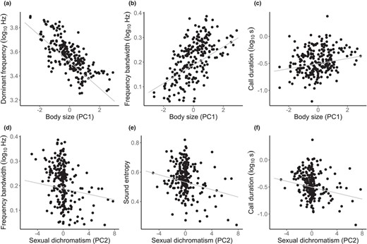
Scatterplots of species values for (a) dominant frequency, (b, d) frequency bandwidth, (c, f) call duration or (e) sound entropy, on (a–c) body size or (d–f) sexual dichromatism across parrot species. Regression lines from the model‐averaged PGLS models are shown in grey. Body size is the first Principal Component (PC) of a Principal Component Analysis (PCA) on morphological measurements, and sexual dichromatism is the second PC of a PCA on plumage colour measurements (see Section 2)
Four phylogenetic generalized least squares (PGLS) regression models of an acoustic trait on morphological and ecological predictors
| Dominant frequency (model λ = 0.85 [0.75, 0.89], = 0.34) | Frequency bandwidth (model λ = 0.75 [0.62, 0.81], = 0.20) | Sound entropy (model λ = 0.81 [0.66, 0.84], = 0.04) | Call duration (model λ = 0 [0.00, 0.00], = 0.12) | |||||||||
| β st | p | 95% CI | β st | p | 95% CI | β st | p | 95% CI | β st | p | 95% CI | |
| Body size | −0.67 | <0.01 | [−0.80, −0.53] | 0.45 | <0.01 | [0.30, 0.61] | −0.17 | 0.10 | [−0.38, 0.04] | 0.21 | <0.01 | [0.07, 0.35] |
| Habitat | 0.04 | 0.71 | [−0.06, 0.08] | 0.04 | 0.41 | [−0.05, 0.12] | 0.06 | 0.30 | [−0.05, 0.17] | 0.09 | 0.15 | [−0.03, 0.22] |
| Gregariousness | 0.01 | 0.75 | [−0.06, 0.08] | −0.03 | 0.44 | [−0.12, 0.05] | 0.04 | 0.54 | [−0.08, 0.15] | 0.06 | 0.37 | [−0.07, 0.18] |
| Ornamentation | 0.02 | 0.67 | [−0.06, 0.10] | 0.02 | 0.75 | [−0.08, 0.12] | 0.01 | 0.87 | [−0.12, 0.14] | −0.10 | 0.12 | [−0.23, 0.03] |
| Dichromatism | 0.01 | 0.83 | [−0.08, 0.10] | −0.12 | 0.04 | [−0.22, −0.01] | −0.21 | <0.01 | [−0.35, −0.06] | −0.21 | <0.01 | [−0.34, −0.07] |
Model λ: phylogenetic signal of the PGLS model, followed by its 95% confidence interval; : variance explained by the five predictor traits; β st: standardized partial regression coefficient of predictor; 95% CI: 95% confidence interval of β st.
Inter‐quartile frequency bandwidth was also associated with body size (β st = 0.45, p < 0.001; Figure 2b), with larger species using wider frequency bandwidths, and there was a marginally significant negative association with sexual dichromatism as well (β st = −0.12, p < 0.05; Figure 2d); habitat, gregariousness and overall colour ornamentation did not predict frequency bandwidth (all |β st| < 0.05, all p > 0.44; Table 2). The model was 0.20 and, as can be seen by β st values in Table 2, this explained variation was mostly because of the effect of body size and to a smaller extent that of sexual dichromatism. When analysing MaxMin bandwidth instead of inter‐quartile bandwidth, the effect of body size remained statistically significant, but not that of sexual dichromatism (Table S3).
The sound entropy of calls, which indicate harmonically complex or noisy sounds, was negatively associated to sexual dichromatism (β st = −0.21, p < 0.01; Figure 2e), and was not predicted by body size, habitat, gregariousness or overall colour ornamentation (all |β st| < 0.05, all p > 0.10; Table 2). The model was 0.04 and, as indicated by β st values in Table 2, this explained variation was mostly because of the effect of sexual dichromatism followed by that of body size, albeit the latter not being statistically significant.
Finally, call duration was positively associated to body size (β st = 0.21, p < 0.01; Figure 2c) and negatively associated to sexual dichromatism (β st = −0.21, p < 0.01; Figure 2f), although it was not predicted by habitat type, gregariousness or colour ornamentation (all |β st| < 0.09, all p > 0.12; Table 2). The model was 0.12, and this explained variation was because of similarly strong effects of body size and sexual dichromatism (Table 2). Unlike the three previous PGLS models, which all had high values of λ (≥0.75 in all cases; Table 2), indicating phylogenetic structure for the residual variation in acoustic traits, the PGLS model on call duration had an estimated λ = 0, which may reflect the fact that call duration had the lowest phylogenetic signal of all acoustic traits (λ = 0.14, all other λ ≥ 0.77; see above).
DISCUSSION
Our study of species differences in the duration and sound frequency of parrot calls indicated that body size and sexual selection have exerted stronger influences on call evolution than habitat type or gregariousness. We found that associations with body size pervasively influenced the evolution of parrot calls (call duration, sound frequency and frequency bandwidth), and we did not find species differences in call duration or in sound frequency traits between species from forested versus non‐forested habitats, nor between more and less gregarious species. Interestingly, we found negative associations between sexual dichromatism and several aspects of call complexity (frequency bandwidth, sound entropy and duration), as predicted by the transference hypothesis for the evolution of multiple sexually‐selected signals.
The effects of body size that we found on acoustic properties of parrot calls confirm and expand knowledge of how body size influences vocal signals. First, it has long been known that larger species on average use lower‐frequency sounds (Gingras et al., 2013; Martin et al., 2017; Wallschläger, 1980), because their larger vocal organs and vocal tracts allow producing, resonating and broadcasting low frequencies more efficiently (Bradbury & Vehrencamp, 2011; Fletcher, 2004). Our results, together with those of Medina‐García et al., (2015) for neotropical parrots, confirm this pattern for parrot calls. Second, sound frequency bandwidth is also predicted to correlate with body size because, although efficient use of low frequencies is limited by the size of the vocal apparatus, frequency can be modulated upwards by applying force to the vibrating sound‐producing structures (Elemans et al., 2009; Titze & Martin, 1998) and/or increasing resonant frequencies by contraction of the vocal tract (Bradbury & Vehrencamp, 2011; Goller & Riede, 2013). This may cause that larger species are able to use wider frequency bandwidths, comprising both low and high frequencies in the hearing range, than smaller species, restricted to the higher frequencies. This association between frequency bandwidth and body size was recently reported for songs across passerine birds (Friis, Sabino, et al., 2021), and our results show that it exists for parrot calls too. Contrary to our result and to the theoretical prediction, an earlier study across neotropical parrots (Medina‐García et al., 2015) reported a negative association between frequency bandwidth and body size (i.e. wider frequency ranges in smaller rather than in larger species). That earlier result may be because of frequency bandwidth having been computed as a difference of frequencies on a linear scale, as opposed to on a ratio scale, thus overestimating bandwidth in species using high frequencies (mostly small‐sized species) relative to species using low frequencies (mostly large‐sized species). Frequency bandwidth should instead be computed as frequency ratios or, equivalently, as differences on a logarithmic scale, which corresponds to how animals perceive frequency changes and how they modulate resonant frequencies (Cardoso, 2013), solving the above bias. Third, we found that larger species on average have longer calls, as predicted by their larger air‐sacs and ventilator capacity. A similar result was reported for the duration of songs or notes in passerines (Badyaev & Leaf, 1997; Price & Lanyon, 2004) or of vocalizations across some non‐passerine birds (Gonzalez‐Voyer et al., 2013), including neotropical parrots (Medina‐García et al., 2015).
Our results suggest that the AAH was not a major influence for the evolutionary divergence of acoustic signals across parrot species. Sound attenuation and degradation differ between closed and open habitats, and the AAH thus predicts that, to maximize sound transmission, closed‐habitat species should evolve lower‐frequency vocalizations and narrower frequency bandwidths and use longer notes (Blumenrath & Dabelsteen, 2004; Graham et al., 2017; Hansen, 1979; Morton, 1975; Wiley & Richards, 1978). However, similarly to previous results for neotropical parrots (Medina‐García et al., 2015) and to recent comparative work across passerine birds (Friis, Dabelsteen, et al., 2021; Mikula et al., 2020), we found no evidence that parrot species living mostly in closed habitats differ from those living mostly in open habitats neither on sound frequency, frequency bandwidth nor call duration. Parrots are very mobile, and many species, although having a preferred habitat, can move between closed and open habitats, or forest species may fly and vocalize at different heights in or above the canopy (Gilardi & Munn, 1998), which contributes to make our test of the AAH conservative. But, even using a conservative test, if the AAH was important for the evolution of differences in calls among parrots, our large‐scale comparison (>200 species) should afford statistical power to detect at least suggestive associations with habitat, which was not the case in our results.
We also found no evidence that gregarious species have more complex calls, on any aspect of call complexity that we studied: frequency bandwidth, sound entropy or call duration. The social complexity hypothesis predicts that gregarious species evolve a more complex signalling system, to accommodate the greater diversity of messages and/or to distinguish among a larger number of individuals in a group (Freeberg, 2006; Freeberg et al., 2012), and these functions might be accomplished via the aspects of call complexity that we studied here. For example, individuality in parrot calls can be achieved by among‐individual differences in call frequency and duration (Thomsen et al., 2013; Wanker & Fischer, 2001), suggesting that more complex calls in the frequency or time domains could allow distinguishing among a larger number of group members. We note, however, that here we did not study call repertoire size, and that repertoire size is the vocal trait most often differing between simple and complex animal societies (reviewed in Freeberg & Krams, 2015, and Leighton & Birmingham, 2021, for passerine birds, and in McComb & Semple, 2005, for primates). Parrots can have complex vocal repertoires (e.g. Martins & de Araujo, 2020), as expected for a social species. We focused only on characterizing the most common call of each species, in order to characterize how each species most commonly sounds like, and also because the number and quality of acoustic recordings available in repositories is insufficient to characterize call repertoires for most parrot species. A limitation of this procedure is that we cannot analyse repertoire sizes, nor distinguish evolutionary patterns between calls with specific functions (e.g. aggressive, appeasement or alarm calls). Therefore, although we found no support for the social complexity hypothesis in relation to the acoustic complexity of the main call types of each parrot species, a definitive assessment of the importance of this hypothesis needs further work focusing on vocal repertoires.
Finally, we found that more male‐biased sexually dichromatic parrot species, whereby males have more elaborate or diverse ornamentation than females, have simpler calls on all aspects of call complexity that we studied: narrower frequency bandwidth, lower sound entropy and shorter duration. We found these associations with call complexity when studying male‐biased sexual dichromatism, but not when studying the overall elaboration of colour ornamentation, both of which are commonly used as proxies for the strength of sexual selection on ornamentation. These two proxies have different advantages and disadvantages. Sexual dichromatism has the advantage of being easier and more objective to compute compared to cross‐species scores of colour elaboration, because conspecific males and females usually differ only in the degree to which they express an identical pattern of ornamentation, and different species often differ on multiple aspects of ornamentation that are difficult to integrate and compare in a biologically‐relevant manner. This is an important advantage because, for example, plumage coloration in different body parts of parrots may have different functions and patterns of evolution (Merwin et al., 2020). Moreover, different colours or body parts may also differ in the degrees to which they evolve sexual dichromatism (Taysom et al., 2011), all of which complicate the comparison of ornamentation, especially between species differing strongly in their pattern of plumage colour ornamentation. Sexual dichromatism has the disadvantage that it can evolve as a result of different causes, not all related with stronger sexual selection on males (Price, 2019), and that, although high male‐biased dichromatism indicates elaborate male ornamentation, low dichromatism can indicate different things (either both sexes being very or little ornamented; e.g. Hofmann et al., 2008; Price & Eaton, 2014). This introduces noise when using dichromatism as a proxy for sexual selection and, therefore, likely underestimates how strongly sexual selection affects call evolution.
Despite having both advantages and disadvantages as a proxy for the strength of sexual selection on ornamentation, sexual dichromatism has been found to be a more useful tool in comparative work with bird species than overall colouration scores (Dunn et al., 2015; see also discussion in Cooney et al., 2018). As male‐biased sexual dichromatism is generally a useful proxy for strong sexual selection on male ornamentation, our results with parrots indicate a negative correlation between the evolution of elaboration in visual and acoustic signals. This is consistent with the transference hypothesis among sexual signals (Gilliard, 1956; Johnson, 1999; Schluter & Price, 1993), according to which strong sexual selection for one type of signal reduces selection for elaboration of a different type of signal or, as originally formulated by Darwin (1871), constraints on the evolution of one type of signal increase selection for elaboration of a different type of signal. The proportion of variation explained in models of call complexity (frequency bandwidth, sound entropy or call duration) was never large, varying from 4% to 21%, and in most cases body size was the most important or single significant predictor of acoustic differences between parrot species. Nonetheless, for some acoustic traits (sound entropy and call duration), the effect of sexual dichromatism was as strong or stronger than that of body size (cf. β st values in Table 2). Note also that measures of male‐biased sexual dichromatism provide only a coarse index to the strength of sexual selection on male ornamentation, as explained above, and therefore likely underestimate the strength of the negative correlation between the elaboration of visual and acoustic signals.
The transference hypothesis has been much investigated in birds, with comparative studies reporting a mixture of positive correlations, no correlations or, very rarely, negative correlations between the elaboration of visual and vocal signals (e.g. no correlation: Gomes et al., 2017; Mason et al., 2014; Matysioková et al., 2017; Ornelas et al., 2009; positive correlation: Catchpole & McGregor, 1985; De Repentigny et al., 2000; Gonzalez‐Voyer et al., 2013; Ligon et al., 2018; Shutler & Weatherhead, 1990; negative correlation: Badyaev et al., 2002; Shutler, 2011). With few exceptions, the reason for these different results is unclear (Shutler, 2011). For example, one such exception is the birds‐of‐paradise, where acoustic and visual signals evolved in a positively correlated manner because they are integrated in courtship rituals (Ligon et al., 2018). Another example is that of estrildid finches, where song and colour ornamentation are uncorrelated but where each type of signal evolves associated with different socio‐ecological factors (Gomes et al., 2017), suggesting that whether and how different signals are correlated may depend on how their socio‐ecological predictors are co‐distributed across species. Our work is one of the largest‐scale comparative tests of the transference hypothesis for acoustic and visual signals, and one of the rare studies supporting its main prediction. Our results indicate that sexual selection influenced the evolution of species differences in acoustic signals among parrots, in some traits on par with the effects of body size, whereas, by comparison, the acoustic adaptation and social complexity hypotheses did not have a major influence on the evolution of these species differences in acoustic signals.
ACKNOWLEDGEMENTS
For this study, FM and JS were funded by FEDER Funds through the Operational Competitiveness Factors Program “COMPETE”, and by National Funds through the Foundation for Science and Technology (FCT) within the framework of project ‘PTDC/BIA‐ECO/30931/2017‐POCI‐01‐0145‐FEDER‐030931’. GCC and LR were supported by Portuguese National Funds through FCT, I.P. (DL57/2016/CP1440/CT0011 and CEECIND/00445/2017, respectively). We thank Vicente García‐Navas and one anonymous reviewer for their helpful comments. We also thank Rita Silvestre for the help with the graphical abstract.
CONFLICT OF INTEREST
The authors have no conflict of interest to declare.
AUTHOR CONTRIBUTIONS
JS and LR conceived the original idea with contributions from GCC and FM. GCC, FM, JS and LR designed the study. FM and DB analysed the recordings with support from GCC, JS and LR. GCC designed the analyses with input from FM and JS. FM and GCC conducted the analyses and interpretations with input from JS. FM wrote the paper with the assistance of GCC, JS and LR. All the authors read and approved the final version.
PEER REVIEW
The peer review history for this article is available at https://publons.com/publon/10.1111/jeb.13986.
DATA AVAILABILITY STATEMENT
The complete dataset used in this study is available in the Dryad repository at https://doi.org/10.5061/dryad.pk0p2ngq6.
REFERENCES
