


Abstract
When environmental conditions differ both within and among populations, multiscale adaptation results from processes at both scales and interference across scales. We hypothesize that within‐population environmental heterogeneity influences the chance of success of migration events, both within and among populations, and maintains within‐population adaptive differentiation. We used a simulation approach to analyse the joint effects of environmental heterogeneity patterns, selection intensity and number of QTL controlling a selected trait on local adaptation in a hierarchical metapopulation design. We show the general effects of within‐population environmental heterogeneity: (i) it increases occupancy rate at the margins of distribution ranges, under extreme environments and high levels of selection; (ii) it increases the adaptation lag in all environments; (iii) it impacts the genetic variance in each environment, depending on the ratio of within‐ to between‐populations environmental heterogeneity; (iv) it reduces the selection‐induced erosion of adaptive gene diversity. Most often, the smaller the number of QTL involved, the stronger are these effects. We also show that both within‐ and between‐populations phenotypic differentiation (Q ST) mainly results from covariance of QTL effects rather than QTL differentiation (F STq), that within‐population QTL differentiation is negligible, and that stronger divergent selection is required to produce adaptive differentiation within populations than among populations. With a high number of QTL, when the difference between environments within populations exceeds the smallest difference between environments across populations, high levels of within‐population differentiation can be reached, reducing differentiation among populations. Our study stresses the need to account for within‐population environmental heterogeneity when investigating local adaptation.
Abstract

INTRODUCTION
The emergence and intensity of local adaptation is one of the oldest questions of evolutionary biology (e.g. Darwin, 1859; Endler, 1977; Kawecki & Ebert, 2004), and its theoretical foundations are well known (Bulmer, 1972; Débarre & Gandon, 2010; Haldane, 1930; Levene, 1953). For quantitative traits under stabilizing selection, individual fitness decreases with phenotypic distance to the local optimum, which prevents the departure of population mean phenotype from this optimum (Slatkin, 1978). When different environments define different optima, local adaptation can result from divergent selection maintaining mean population values near their local optima (Kawecki & Ebert, 2004). Levels of differentiation depend on the difference between local optima and on the intensity of stabilizing selection. Divergent selection is expected among populations, leading to local adaptation sensu stricto, but also within population, leading eventually to another form of local adaptation, often referred to as “microgeographic adaptation” (Richardson et al., 2014). Indeed, despite the intuitive idea that adaptation should be impeded by strong local gene flow, there is increasing empirical evidence that groups of individuals within the reach of gene flow can adapt to microgeographic environmental variations (e.g. Audigeos et al., 2013; Barth et al., 2017; Brousseau et al., 2013, 2021; DeMarche et al., 2016; Gauzere et al., 2020; Jain & Bradshaw, 1966; Lind et al., 2017; Maciejewski et al., 2020; Scotti et al., 2016; Szulkin et al., 2016; Turner et al., 2010). As within‐ and between‐populations scales have generally been considered separately, our objective here is to investigate local adaptation simultaneously at both scales, using simulation experiments in hierarchical population structures where environmental conditions differ both among populations and within each population.
We hypothesize that within‐population environmental heterogeneity influences the chance of success of migration events, both within and among populations; hence, it may contribute to maintaining within‐population genetic variance, simultaneously constraining adaptive differentiation among populations and increasing potential response to selection within population (Barrett & Schluter, 2008). In this sense, within‐population adaptation is a form of balancing selection that can drive evolutionary potential in each population (Delph & Kelly, 2014), which suggests possible cross‐scale interaction of local adaptation processes. So far, hierarchical population structures have been mostly studied in the neutral case as a reference situation to infer selection. Hierarchical gene differentiation parameters at between‐populations and within‐population levels (FRT and FSR, respectively) were defined by Slatkin and Voelm (1991). Whitlock and Gilbert (2012) introduced the corresponding parameters for quantitative traits (QRT and QSR). In a previous study (Cubry et al., 2017), we have shown that both between‐populations and within‐population adaptive differentiation can be inferred when hierarchical Q‐statistics exceed their corresponding Fq‐statistics (i.e. the F‐statistics at the QTL). As hierarchical population structures are a recognized biological reality, the interplay of selection at different levels is still understudied.
At a single geographical level, population responses to selection are well known to depend on selection intensity, trait heritability and population additive genetic variance. Several counteracting forces can prevent populations from reaching their local optima: mutation, genetic drift, gene flow and balancing selection (Yeaman & Otto, 2011). Population responses to these drivers depend on the genetic architecture of traits (Láruson et al., 2020) and on life‐history characteristics, such as mating system (but see Hereford, 2010) and fecundity rate. Regarding genetic architecture in particular, analytical derivations and simulation‐based studies, assuming additive polygenic trait inheritance showed that local adaptation first proceeds by selection of the best local allelic combinations, and then by changes of allele frequencies (Kremer & Le Corre, 2012; Le Corre & Kremer, 2003, 2012; McKay & Latta, 2002). Thus, differentiation measured by Q‐statistics has two components, the divergence of QTL‐allele frequencies (Fq‐statistics) and the covariance of allelic effects among populations, which induces a decoupling between Q‐statistics (differentiation at traits) and Fq‐statistics (differentiation at underlying QTL). Genetic architecture therefore affects evolutionary dynamics, because the larger the number of QTL, the larger the impact of covariance of allelic effects on adaptive differentiation (Latta, 1998; Le Corre & Kremer, 2012). As the way selection affects QTL diversity and divergence is thus fairly well known, the consequences of cross‐scale interactions of selection processes in hierarchical population structures on the distribution of genetic diversity are still largely unknown.
Addressing the outcome on local adaptation of interactions between genetic architecture, gene flow and selection intensity in hierarchical population structures may thus be extremely complicated, and analytical solutions to the problem may not be straightforward. Simulation approaches have the advantage of controlling sources of variation, thus allowing the analysis of the links between processes and patterns. Here, we used a cross‐design simulation experiment to investigate how patterns of within‐ and between‐populations environmental heterogeneity, selection intensity and genetic architecture jointly affect local adaptation, both among populations and between environments within populations. To that aim, we modelled a two‐level metapopulation structure and considered the case of a polygenic trait with different phenotypic optima both among populations and between environments within populations. We used a single, general dispersal scheme including gametic and zygotic dispersal stages.
We computed a panel of criteria accounting for the demographic, phenotypic and genetic dimensions of local adaptation along the environmental gradient. Local adaptation processes can be studied through multiple approaches: by comparing mean population fitness to maximum fitness (Lande, 1976); by computing adaptation lag (the mean difference between realized and optimal phenotypes; Kawecki & Ebert, 2004); by demonstrating clinal adaptive variation across environmental gradients (Endler, 1977); by assessing temporal dynamics in gene and trait diversity, to decipher the respective role of neutral evolutionary forces and selection (Franks & Hoffmann, 2012); and/or by comparing neutral and adaptive genetic diversity and differentiation, in theoretical and simulation studies where the neutral and adaptive genes are controlled. The conditions and outcome of local adaptation are not uniform along the environmental gradient. In particular, the potential for local adaptation at range margins may be constrained by lower adaptive variation (Alleaume‐Benharira et al., 2006), which may ultimately affect survival (Bridle & Vines, 2007). Here, for each environment, (i) we measured occupancy rate as an indicator of successful adaptation; (ii) we quantified the magnitude of adaptation through adaptation lag; (iii) we assessed additive variance as a driver of local adaptive potential. Across the whole range, we characterized the polygenic response to selection by comparing QTL diversity with neutral gene diversity and by comparing hierarchical Q‐statistics with Fq‐statistics.
We compared different environmental heterogeneity patterns with or without within‐population variation, in combination with variations in life‐history parameters (fecundity rate and mating system), to investigate how within‐population heterogeneity affects: (1) the rate of occupancy of the different environments, (2) adaptation lag and genetic variance in the different environments and (3) gene diversity structure across scales. In each case, we analysed whether the effect of within‐population heterogeneity depends on genetic architecture and selection intensity. Taken together, our results allowed us to investigate whether adaptive differentiation proceeds differently at between‐populations and within‐population scales and how local adaptation processes interfere across scales.
MATERIALS AND METHODS
The simulations were run on the Nemo platform v2.3.51 (Guillaume & Rougemont, 2006). Data availability is described in Appendix 1.
Simulation design
We simulated a hierarchical metapopulation with four populations, two environments per population (i.e. eight environments in total, no environmental redundancy between populations) and three patches per environment (i.e. 24 patches in total; Figure 1). We modelled both pre‐ and post‐zygotic gene flows with a single set of gene flow parameters, inspired from pollen and seed‐mediated gene flow estimates in wind‐dispersed trees (Petit et al., 2005). We used a gamete/zygote dispersal ratio of 20. The probability to disperse from one population to another was 0.05 for gametes and 0.0025 for zygotes. Within each population, the probability to disperse from one patch to another was 0.7917 (0.95 × 5/6) for gametes and 0.0416 (0.9975 × 5/6/20) for zygotes. We set the carrying capacity of each patch to 100 individuals.
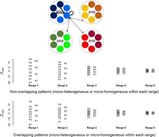
Schematic representation of the hierarchical metapopulation structure with four populations (dotted circles), two environments per population (colours) and three patches per environment (small circles). Migration rates within and between populations were fixed. Environments were characterized by their optimal phenotypic values (Zopt): in the micro‐heterogeneous pattern, Zopt varied between the two environments within each population (i.e. eight Zopt values in total), whereas in the micro‐homogeneous pattern, the two environments had similar Zopt within each population (i.e. four Zopt values in total). We simulated five ranges of Zopt values, and, in the micro‐heterogeneous patterns, Zopt values were either overlapping across populations or not, as shown in the bottom part of the figure (P1 to P4 represent the four populations). Note that micro‐heterogeneous overlapping and non‐overlapping patterns had two different micro‐homogeneous references adjusted to their respective sets of mean Zopt values per population
As an initialization step, we first derived metapopulations at drift‐mutation‐migration quasi‐equilibrium (Appendix 2a). Then, we performed a selection step using a complete factorial design with ten replications of each combination of parameters as indicated in Table 1. We performed in total 19200 simulation runs. Each simulation started from the appropriate initialized data set and was extended with the new parameters of the selection step for 200 generations, which we considered as a realistic time span over which environmental conditions may be considered relatively stable and long enough to get effects of the sets of parameters used. We tracked demographic and genetic statistics over generations and observed that, after 200 generations, demographic and genetic variables had reached, or were very close to, asymptotic values (Appendix 2b). We recorded the individual genotypes over the whole metapopulation after 200 generations for further analyses.
Parameter sets used in the simulations
| Parameter | No of modes | Modes |
| Mutation model | 2 | Diallelic model Continuous, infinite allele model |
| No of QTL | 2 | 10 50 |
| Environmental range | 5 | 1 = [−19.60; +19.60] 2 = [−14.70; +14.70] 3 = [−7.35; +7.35] 4 = [−4.90; +4.90] 5 = [−2.45; +2.45] |
| Environmental pattern | 4 | Non‐overlapping micro‐heterogeneous Non‐overlapping micro‐homogeneous reference Overlapping micro‐heterogeneous Overlapping micro‐homogeneous reference |
| Selfing rate | 2 | 0 0.3 |
| Fecundity | 3 | 10 100 200 |
| Stabilizing selection intensity | 4 | ω 2 = 1 (strong) ω 2 = 5 (moderate) ω 2 = 20 (weak) ω 2 = 50 (very weak) |
| No of scenarios | 1920 | |
| Replicates | 10 | |
| Total no of simulations | 19 200 |
Genetic architecture and mutation models
Based on a genetic map consisting of 10 linkage groups of 170, 80, 150, 90, 60, 90, 50, 70, 110 and 130 cM, respectively, i.e. random lengths for a total length of 1000 cM, we simulated 2000 neutral loci under a diallelic mutation model with a mutation rate of 5 × 10⁻⁵. The loci were uniformly distributed over the genetic map, with an inter‐locus distance of 0.5 cM.
For the trait under selection (directly affecting fitness), we applied two purely additive models of quantitative inheritance, with either 10 or 50 QTL, evenly distributed across linkage groups (i.e. 1 QTL per linkage group in the 10 QTL model, 5 QTL per linkage group in the 50 QTL model). These different genetic architectures are expected to behave differently with regard to the role of covariance among QTL on the genetic variance (Le Corre & Kremer, 2012). QTL positions were randomly chosen within each linkage group once for the whole set of simulations (Appendix 1). For the starting population, QTL allelic effects were randomly drawn from a normal distribution of mean 0 and variance 1 (10 QTL model), or mean 0 and variance 0.2 (50 QTL model), resulting in similar additive variance for the two models in a large initial population where each QTL has two alleles in equal frequencies. Then, during the simulations, each QTL followed either a diallelic mutation model or a continuous, infinite allele mutation model, which are expected to generate different patterns of covariance among QTL allelic effects. The diallelic mutation model used a mutation rate of 5 × 10⁻⁵ per locus per generation that switched the sign of the allelic value leading to positive or negative contribution to the trait. The continuous mutation model used the same mutation rate but here each new mutation changed the initial allelic value by a quantity drawn from a normal distribution of mean 0 and variance 1 or mean 0 and variance 0.2 (10 QTL and 50 QTL models, respectively).
Selection and environmental heterogeneity patterns
After initialization (Appendix 2), we ran the selection step where we applied different levels of stabilizing selection ω2 within each patch based on the individual survival probability computed as , where Z is the phenotype of the individual and Zopt the local phenotype optimum. We simulated four values of selection intensity ω²: 1 (strong), 5 (moderate), 20 (weak) and 50 (very weak).
Zopt values varied between populations and between environments within populations as shown in Figure 1. To simulate different levels of ‘adaptive demand’ during the selection step, we used five different ranges of Zopt values (called ‘environmental ranges’), corresponding respectively to 8, 6, 3, 2 and 1 times the expected phenotypic standard deviation. This means the most extreme environments were from 4 to 0.5 times the phenotypic standard deviation apart from the mean value when the selection step started (mean phenotypic optimum was set to 0 during the initialization step).
For each environmental range, we designed four different patterns of environmental heterogeneity that remained fixed during the selection step (Figure 1): (a) two patterns (hereafter called ‘micro‐heterogeneous patterns’) had within‐population environmental heterogeneity, whereby each population contained two 3‐patch groups having different Zopt values, resulting in eight different Zopt values. In one micro‐heterogeneous pattern, Zopt values overlapped between populations (‘overlapping pattern’), whereas in the other one Zopt values were disjunct (‘non‐overlapping pattern’); (b) two ‘reference’ patterns (thereafter called ‘micro‐homogeneous patterns’) had no within‐population environmental heterogeneity, whereby the unique Zopt value of each population was equal to the mean of the two Zopt values of the corresponding micro‐heterogeneous patterns (this led to two micro‐homogeneous patterns, because the means of Zopt per populations were different in the overlapping and the non‐overlapping designs).
Life cycle
Life cycle events occurred in the following order: mating (including gamete dispersal), zygote dispersal, selection, density regulation to reach the carrying capacity within each patch and, lastly, ageing and death of current adults. This cycle corresponds to a process of ‘compensatory hard selection’, whereby post‐dispersal selection depends on the match between individual phenotypes and the local optimum (hard selection) whereas local density regulation within each patch creates density and frequency‐dependent selection at the global level (following Bell et al., 2021). It mimics a life cycle where only male gametes (e.g. pollen grains) and zygotes (e.g. seeds) disperse, with non‐overlapping generations.
Analysis of simulation outputs
Basic demographic and genetic statistics were directly provided by Nemo both at metapopulation level and for each patch: population density relative to the carrying capacity, gene diversity and differentiation indices for neutral loci and QTL, phenotypic means and genetic variances. We averaged these values over the ten replicates for each set of simulation parameters. We also deemed patches as ‘occupied’ when at least an individual was observed in a patch, and defined an environment (or a population) as occupied when this environment (or population) was represented at least by one occupied patch in one of the ten replicates.
In addition, we used the raw genotypic datasets for each simulation run to compute hierarchical F‐statistics between populations, between environments within populations and between patches within environments within populations following (Yang, 1998). We computed these statistics for the QTL (hierarchical FSTq) and for a subset of 500 neutral markers, evenly spaced in the genome (hierarchical FST), using the varcomp.glob function of the package hierfstat v0.04–22 (Goudet & Jombart, 2015) in R v3.5.2 (R Core Team, 2018). Since measures of between‐deme differentiation based on expected heterozygosity, such as F‐statistics, are not independent from within‐deme diversity (see Lefèvre and Gallais (2020) for review), we also computed Jost's D differentiation, which is independent of within‐deme diversity (Jost, 2007, 2008), and which we extended to a hierarchical population structure (Appendix 3).
We computed the hierarchical variance components of the genotypic value using a linear mixed effects model with nested random effects of patches within environments within populations, in the micro‐heterogeneous patterns, or patches within populations in the micro‐homogeneous patterns, with the lme function of the package nlme v3.1–137 (Pinheiro & Bates, 2000) in R v3.5.2. We then computed the hierarchical Q‐statistics at population, environment and patch levels following Cubry et al. (2017). The comparison of the Q‐statistics and the Fq‐statistics, i.e. the F‐statistics at the QTL, provides information on the respective role of covariance among QTL allelic effects and divergence of QTL‐allele frequencies in the process of adaptation. To quantify this effect, Gavrilets and Hasting (1995) introduced a parameter θ that represents the part of the additive variance due to the covariance of allelic effects among QTL relative to the part of the variance due to the sum of individual allelic effects. In a simple population structure for the diallelic case, Le Corre and Kremer (2003) had given the relationship between Q ST and F STq in terms of θST and θIS (respectively the between‐ and within‐deme covariance parameters). They showed that (i) QST equals FSTq when the covariance correction terms between and within deme are equal, even if not null, and (ii) QST exceeds FSTq when the covariance of allelic effects is higher between demes than within demes, as expected under divergent selection. We generalized this analytical development to the case of hierarchical population structures in the diallelic mutation model (Appendix 3). In a hierarchical structure, our developments show that conditions leading to equality between hierarchical Q‐statistics and Fq‐statistics are more complex but still, equality is achieved when all covariance components are null or equal across scales (Appendix 3). Analytical developments are not available for the continuous mutation model but the discrepancy between Q‐statistics and Fq‐statistics informs on the role of covariance of allelic frequencies beyond the effect of divergence of allelic frequencies in the adaptation process.
RESULTS
The overall effects of evolutionary parameters on demographic and genetic diversity variables are shown in Appendix 4. Below, we detail some results from simulations performed with: diallelic mutation, no selfing and fecundity rate equal to 200. Other cases are reported as supplementary material using a graphical layout similar to the main texts (Appendix 5).
Effect of within‐population environmental heterogeneity on the rate of patch occupancy
In our model, the rate of patch occupancy depends both on the zygote migration rate and on selection (which can ultimately eliminate all the individuals of a given patch, including migrants). Under weak and very weak selection (ω² = 20 and 50), all patches were occupied irrespective of within‐population environmental heterogeneity (Figure 2 and Appendix 5‐Fig S2). With strong and moderate selection intensities (ω² = 1 and 5 respectively) and the widest environmental ranges, however, we observed contrasting results between simulations with vs. without within‐population environmental heterogeneity (Figure 2). In the micro‐homogeneous patterns, patches at the margins of the environmental range remained unoccupied whatever the genetic architecture. The micro‐heterogeneous patterns allowed higher rates of patch occupancy in these environments, and all extreme patches were occupied in the 50 QTL cases but not in the 10 QTL cases.
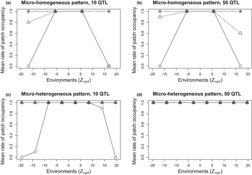
Mean rates of patch occupancy per environment in the widest range of Zopt values (range 1), depending on environmental heterogeneity pattern (a‐b: micro‐homogeneous; c‐d: micro‐heterogeneous), genetic architecture(a‐c: 10 QTL; b‐d: 50 QTL) and selection intensity (circle: strong ω²=1; triangle: moderate ω² = 5; + sign: weak ω² = 20; x sign: very weak ω² = 50). Rates were averaged over 10 replicated simulations. Results shown for non‐overlapping patterns
The effect of population heterogeneity on the rate of patch occupancy also depended upon the interaction of selection intensity and range of optimal phenotypic values (Zopt). In the case of the widest range (range 1), strong selection (ω² = 1) made each environment impassable for immigrant phenotypes adapted to other patches—or said otherwise, any phenotype having non‐zero fitness in any given environment had zero fitness in all others (non‐overlapping micro‐heterogeneous patterns shown in Figure 3, other cases in Appendix 5‐Fig S3). The situation became increasingly permissive with weaker selection for both environmental patterns, except at the margins, where immigrants were more at disadvantage with overlapping than with non‐overlapping patterns (Appendix 5‐Fig S3): this was, by design, caused by the larger gap in Zopt between the most extreme environments and the others in the overlapping than in the non‐overlapping patterns (Figure 1). For milder selection intensities, border effects are thus expected to be stronger in the overlapping patterns. In the case of the narrowest range (range 5), weaker stabilizing selection intensity levels mean that most phenotypes have substantial fitness in most environments (Figure 3). The situation is intermediate for ranges 2 through 4 (Appendix 5‐Fig S3).
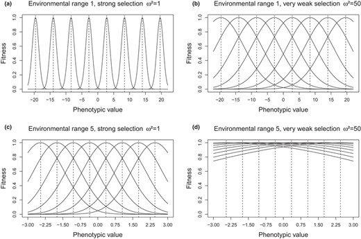
Fitness decrease around the optimum phenotypic values of each environment for two ranges of Zopt values (a‐b: wide range 1; c‐d: narrow range 5), and for two selection intensities (a‐c: strong ω² = 1; b‐d: very weak ω² = 50). Results shown for the micro‐heterogeneous non‐overlapping patterns
Effect of within‐population environmental heterogeneity on adaptation lag and genetic variance along the environmental range
Figure 4a,b shows the adaptation lag (i.e. the offset, in absolute value, between mean observed trait value and the theoretical optimum in a given environment) in the different environments in the widest range of environmental conditions with non‐overlapping heterogeneity (range 1). In this highly selective context, with 10 QTL, the adaptation lag showed U‐shaped patterns, with much larger lags in the marginal environments (Figure 4a). The adaptation lag was globally stronger for all environments in the micro‐heterogeneous than in the micro‐homogeneous patterns (Appendix 5‐Fig S4), and much stronger in the marginal environments. A higher number of QTL (50 QTL) drastically reduced the adaptation lag in the most marginal environments but did not change the adaptation lag in the rest of the metapopulation (Figure 4b). This strong effect of genetic architecture on the adaptation lag in the margins was weaker in narrower environmental ranges (Appendix 5‐Fig S4). In the overlapping pattern, all values of adaptation lag were globally higher than in the non‐overlapping pattern, but the effect of genetic architecture at the margins remained the same (Appendix 5‐Fig S4).
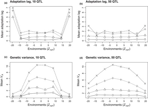
Mean adaptation lag (a‐b) and genetic variance (c‐d) per environment, depending on the genetic architecture (a‐c: 10 QTL; b‐d: 50 QTL) and selection intensity (circle: strong ω²=1; triangle: moderate ω² = 5; + sign: weak ω² = 20; x sign: very weak ω² = 50). Results are shown in the micro‐heterogeneous non‐overlapping pattern with the widest range of Zopt values (range 1). Note that, with this environmental pattern, the case with 10 QTL and very strong selection did not allow the colonization of all patches in the extreme environments (mean values not represented in these extreme situations). Values were averaged over 10 replicated simulations
Within‐environment additive variance VA had a dome‐shaped pattern when plotted against Zopt for all combinations of environmental heterogeneity and genetic architecture (case of the widest range with non‐overlapping microheterogeneity shown in Figure 4c,d, other cases in Appendix 5‐Fig S4): marginal environments systematically had lower variance, although the difference between central and marginal environments depended upon the intensity of selection (with weaker selection allowing for much higher variance in the central environments). Within‐environment additive variance was much more depressed at environmental margins with 10 QTL than with 50 QTL (Figure 4); the reduction in variance from central to marginal environments was stronger in micro‐heterogeneous than in micro‐homogeneous patterns (and more so for 10 than for 50 QTL; Appendix 5‐Fig S4).
The effects of genetic architecture on the adaptation lag and additive variance described above were stronger for the widest range (range 1), but tapered off in narrower ranges (Appendix 5‐Fig S4).
Effect of within‐population environmental heterogeneity on genetic diversity and structure
Figure 5 focuses on QTL diversity and range 3, which is the widest environmental range allowing occupancy of all patches whatever the selection intensity, in combination with the 50 QTL case (see Appendix 5‐Fig S5 for other cases). The very low FST values reached with the weakest selection intensity (ω² = 50) indicate that 200.000 generations of initialization with the same migration rates before applying selection did not result in neutral divergence between populations.
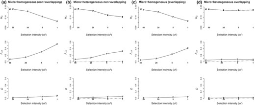
Response of QTL diversity (HS) and differentiation (FST, Jost's D) parameters to selection intensity depending on environmental heterogeneity (a‐c: micro‐homogeneous patterns, two types as shown in Figure 1; b‐d: micro‐heterogeneous patterns). Hierarchical levels are as follows: between populations (p) and between environments within populations (e). The pi indicates the HS values at population level after initialization before divergent selection started. We show averaged values over 10 replicated simulations in the widest range of Zopt values allowing colonization of all patches (range 3) and 50 QTL case
The reduction of genetic diversity at QTL (HSq) in response to selection intensity was less severe in the micro‐heterogeneous than in the micro‐homogeneous pattern, and even no loss of QTL diversity was observed in the overlapping pattern of heterogeneity (Figure 5). In the micro‐heterogeneous patterns, genetic differentiation between environments within populations was almost null, due to within‐population gene flow. Similar levels of diversity (HS or HSq) were therefore observed at population and environment scale, i.e. each environment carried the whole gene diversity of its population, for both neutral loci and QTL (Figure 5, Appendix 5‐Fig S5).
Neutral FST between populations was basically unaffected by selection, whereas for QTL, FSTq increased with selection intensity in all instances. Yet, this increase in FSTq was partly caused by reduction of within‐population HSq rather than by divergence in QTL‐allele frequencies: Jost's Dq, which is independent of heterozygosity, was much less sensitive than FSTq to selection intensity (Figure 5). With overlapping within‐population environmental heterogeneity, lack of response of QTL diversity to selection resulted in lack of response of FSTq.
Selfing reduced within‐population and within‐environment gene diversity, both at neutral loci and QTL (H S and H Sq). In addition, selfing specifically strengthened selection‐induced QTL differentiation between environments within populations (D qenv). These two effects resulted in higher levels of QTL differentiation between environments (F STqenv) with selfing than without selfing, but left neutral differentiation unchanged in most cases (Appendix 5‐Fig S5).
Total additive variance has three hierarchical components: among populations, between environments within populations and among patches within environments. In all cases, increasing selection intensity reduced the within‐environment component and increased both the between‐populations component and the total variance (Figure 6). In overlapping micro‐heterogeneous patterns, the increase in between‐environments variance in response to selection intensity more than compensated the reduction of between‐populations and within‐environment variance components, resulting in higher total variance at metapopulation level at higher selection intensities (Figure 6c,d). Conversely, non‐overlapping micro‐heterogeneous patterns did not show any significant change in the different variance components compared with the micro‐homogeneous reference (Figure 6a,b). As an important factor of adaptive potential, the within‐population variance, which combines both between‐ and within‐environment components, was higher with overlapping within‐population environmental heterogeneity than in all other cases. Moreover, with overlapping patterns, it increased with selection intensity (Figure 6c,d, where within‐population variance can be visualized as the offset between the total and the among population curves).
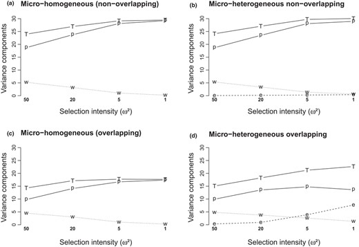
Response of the hierarchical genetic variance components to selection intensity, depending on environmental heterogeneity patterns (a‐c: micro‐homogeneous patterns, two types as shown in Figure 1; b‐d: micro‐heterogeneous patterns). Variance components are as follows: total (T), between populations (p), between environments within populations (e) and within environments (w, includes within‐ and between patch components). We show averaged values over 10 replicated simulations in the widest range of Zopt values allowing colonization of all patches (range 3) and 50 QTL case
Hierarchical Q‐statistics and Fq‐statistics among populations and between environments within populations increased with the intensity of selection, and the decoupling between Q‐statistics and Fq‐statistics revealed the major role played by covariance among allelic effects in adaptation at both scales (Figure 7 and Appendix 5‐Fig S7). At population scale, adaptation led to high QST values (QSTpop >0.6) even under very weak selection (ω² = 50) whereas QTL frequencies remained poorly differentiated in this case (FSTqpop >0.2). FSTqpop was more sensitive to selection intensity than QSTpop, which quickly reached an asymptotic value. Population‐level adaptation in micro‐heterogeneous patterns led to the same levels of QSTpop but to lower levels of FSTqpop than in micro‐homogeneous patterns. QSTpop showed the same response to selection irrespective of genetic architecture, but FSTqpop was less sensitive to selection intensity with 50 QTL.
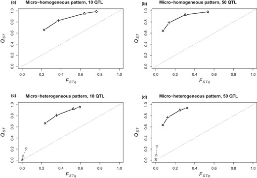
Decoupling between hierarchical Q‐statistics and Fq‐statistics between populations (bold signs and lines) and environments within populations (plain signs and dashed lines), depending on environmental heterogeneity (a‐b: micro‐homogeneous; c‐d: micro‐heterogeneous non‐overlapping pattern), genetic architecture (a‐c: 10 QTL; b‐d: 50 QTL) and selection intensity (circle: strong ω²=1; triangle: moderate ω² = 5; + sign: weak ω² = 20; x sign: very weak ω² = 50). The couples {QST‐FST} follow a concave relationship when selection varies. We show averaged values over 10 replicated simulations in the widest range of Zopt values allowing colonization of all patches (range 3)
In the non‐overlapping heterogeneity patterns, within‐population, environment‐level adaptation only occurred when selection intensity was strong or moderate (ω² = 1 or 5) and moderate QSTenv values were reached whereas FSTqenv values remained very low (QSTenv <0.3, FSTqenv <0.05; Figure 7). Much higher values of QSTenv could be reached, comparable to the QSTpop values or even higher, in the overlapping environmental heterogeneous‐population patterns and with the continuous mutation model (Appendix 5‐Fig S7).
In general, population‐level and within‐population, environment‐level Q‐statistics and Fq‐statistics followed the same concave relationship, whereby low levels of selection increased QST values but higher selection intensity is required to increase FSTq (Appendix 5‐Fig S7). As a general trend, this concave relationship, i.e. the decoupling between Q‐statistics and Fq‐statistics, was more pronounced with 50 QTL than with 10 QTL (Figure 7) and increased with environmental range width (Appendix 5‐Fig S7). We detected a difference between population scale and within‐population, environment‐level responses to divergent selection with regard to the decoupling between Q‐statistics and Fq‐statistics: when stabilizing selection intensity increased (and/or when environmental range became wider), local adaptation at population scale increased FSTqpop more than QSTpop, thus reducing the decoupling, whereas within‐population, environment‐level adaptation increased QSTqenv more than FSTenv, thus increasing the decoupling (Figure 7, Appendix 5‐Fig S7).
Interference between adaptation processes at population scale and within‐population, environment‐level scale occurred mainly in the overlapping micro‐heterogeneous patterns and was particularly clear in the environmental range 2 as illustrated on Figure 8. When the environment was homogeneous within populations, increasing selection intensity resulted in increased between‐population variance and therefore increased QSTpop and FSTqpop. An opposite trend was observed when the environment was heterogeneous within populations: increasing selection intensity resulted in reduced between‐population variance correlated to increase between‐environments within‐population variance, thus decreased QSTpop and increased QSTenv, with almost no response of FSTqpop whereas FSTqenv increased. In addition, in this case, total variance increased in the micro‐heterogeneous case as soon as selection operated. By contrast, compared to their micro‐homogeneous reference patterns, the non‐overlapping micro‐heterogeneous patterns could reach high levels of within‐population differentiation (QSTenv) that did not reduce the level of differentiation between populations (QSTpop, e.g. in the case of range 2 and 50 QTL Appendix 5‐Fig S7).
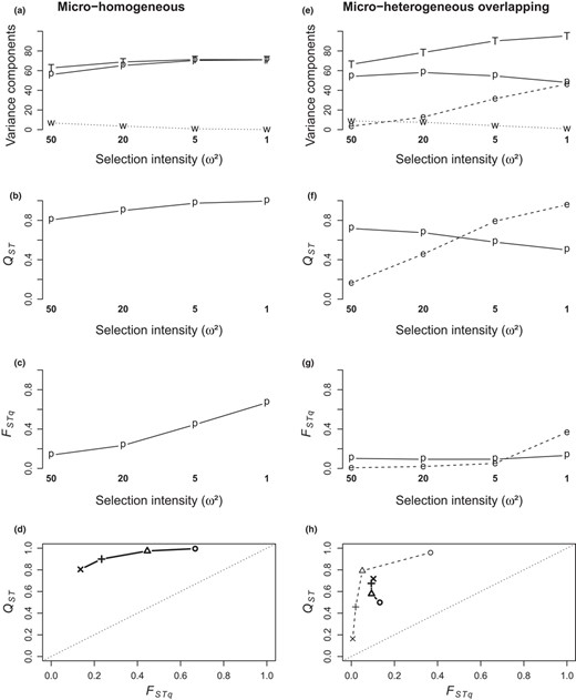
Cross‐scale interference on the response of variance and differentiation parameters to selection intensity (compiled from Appendix 5‐Figs S6 & S7). This interference is illustrated on right column (e‐h) corresponding to the micro‐heterogeneous overlapping pattern, by reference to the left column (a‐d) corresponding to the micro‐homogeneous pattern; other parameters are common to all plots (diallelic mutation, 50 QTL, fecundity 200, no selfing, environmental range 2). Plots on the top three rows (a‐c, e‐g) show the hierarchical components of variance, Q‐statistics and Fq‐statistics (total (T), between populations (p), between environments within populations (e, when applicable), within environments (w)); selection intensity is given on the x‐axis. Plots on the bottom row (d, h) show the decoupling between hierarchical Q‐statistics and Fq‐statistics between populations (bold symbols and bold, full lines) and between environments within populations (plain symbols and plain, dashed lines), depending on selection intensity (circle: strong, ω²=1; triangle: moderate, ω² = 5; “+” sign: weak, ω² = 20; “x” sign: very weak, ω² = 50)
DISCUSSION
Within‐population environmental heterogeneity affects population demography and evolutionary potential
By comparing hierarchical population structure including or not within‐population environmental heterogeneity, we shed new light on the impact of within‐population environmental heterogeneity on multiscale adaptation, within and among populations. We first showed that within‐population environmental heterogeneity globally increases population occupancy at the margins of distribution ranges, under extreme environments and high levels of selection. This is likely due to the higher survival probability of migrants in micro‐heterogeneous than in micro‐homogeneous patterns, for two reasons (which cannot be disentangled here): phenotypic optima of neighbouring environments are closer to each other in micro‐heterogeneous than in micro‐homogeneous patterns, which increases the chance of immigrants getting established; in addition, the larger number of local optima increases the cumulative survival probability of immigrant phenotypes. Increased immigrant survival particularly benefits marginal populations, which undergo high selection demands on migrants (Alleaume‐Benharira et al., 2006; Lenormand, 2002). Survival despite higher adaptation lag in marginal conditions is favoured in a ‘compensatory hard’ selection regime whereby density regulation occurs locally within each patch, as we used here, avoiding overflow of immigrants unfit to marginal conditions that might occur in case of density regulation at global level.
This study also highlights antagonistic effects of within‐population environmental heterogeneity on within‐population additive variance, which is a main driver of the evolutionary potential of a population. In the non‐overlapping micro‐heterogeneous patterns, there is almost no between‐environments variance within each population, because within‐population dispersal efficiently mixes phenotypes selected in different environments. Here, within‐population environmental heterogeneity does not increase within‐population variance, and higher selection intensity leads to lower within‐population variance. We detected an opposite trend in the overlapping micro‐heterogeneous patterns, where stronger selection resulted in higher levels of between‐environments, within‐population variance. Indeed, in the overlapping pattern, inter‐population dispersal brings ‘intermediate’ phenotypes to each population, which can amplify the within‐population balancing selection process more efficiently than in the non‐overlapping pattern, for two reasons. Firstly, the fitness functions within each population are more disconnected from each other in the overlapping pattern, which offers a broader range of phenotypic values with a non‐null survival probability than in the non‐overlapping pattern. Secondly, in the overlapping pattern, a fraction of the inter‐population immigrants’ have intermediate phenotypes between the recipient population's local optima, and thus better match the recipient population's local optima; this contrasts with the non‐overlapping pattern where all immigrants systematically contribute to push the mean phenotypic value of the recipient population away from its optimum. This influx of intermediate phenotypes from another population may strengthen the effect of ‘spatial autocorrelation of selection’ described in Richardson et al. (2014), whereby non‐random patterns of environmental heterogeneity may increase the selective advantage of migrants.
Hence, the sole presence of environmental heterogeneity and multiple optima within a population does not guarantee higher levels of genetic variance. The increase in within‐population variance directly results from the effectiveness of within‐population adaptive divergence and subsequent balancing selection, which requires two conditions: highly contrasted environments within the population and successful inter‐population migration supplying gene diversity. Similarly, in the case of temporal balancing selection, Kondrashov and Yampolsky (1996) showed that the increase in within‐population variance depends on the amount and period of changes in fitness optimum.
Genetic architecture affects multiscale adaptation processes, whereas selfing has a limited impact
Le Corre and Kremer (2012) showed that local adaptation is mainly driven by genetic covariance of allelic effects among QTL and that a higher number of QTL causes a stronger decoupling between QST and FSTq. Here, we generalized this result for multiscale adaptation: both at within‐ and between‐populations scales, local adaptation is mainly driven by the covariance of allelic effects and much less by allelic differentiation. The predominance of the covariance of allelic effects is more pronounced at the within‐population scale (where FSTqenv is negligible) and, as a consequence, higher levels of within‐population adaptive differentiation (QSTenv) are reached with 50 than with 10 QTL, for the same level of QTL differentiation (FSTqenv).
Our results highlight that the number of QTLs drives the adaptive capacity at the environmental margins, where we observed that a higher number of QTL results in a smaller adaptation lag and higher genetic variance. These two intertwined patterns can explain the greater occupancy rates we observed in simulations with 50 QTL versus 10 QTL. This is likely because allele fixation with a 10 QTL architecture has a higher impact on genetic mean and variance than with 50 QTL, resulting in more difficulties to approach the local optimal phenotype. Even though we can hardly know the exact number of QTL controlling a trait in empirical studies, our results point to the value of comparing the genetic architecture of traits between marginal versus core populations across the environmental niche.
Our study also revealed a weak effect of the mating system on local adaptation, consistently with empirical studies (Hereford, 2010). Still, our results suggest that the mating system could interact with selection in the multiscale adaptation process itself, since selfing increased the QTL differentiation at the within‐population scale but had no such effect on QTL differentiation at the between‐populations scale over the evolutionary timescale considered here.
Cross‐scales interferences in within‐ and between‐population adaptation
We showed that at population scale, local adaptation is characterized by adaptive differentiation (QSTpop) and reduced adaptation lag in all cases, even when the environmental contrast between populations is low (i.e. narrow range) and when selection intensity is very weak. Thus, population‐level adaptation is favoured by limited gene flow and does not require strong divergent selection. By contrast, at within‐population scale, adaptive differentiation (QSTenv) only occurs when the contrast between environments within populations is large, and strong selection is required to reduce the adaptation lag. Thus, within‐population adaptive divergence proceeds through strong divergent selection favoured by gene flow that provides the necessary genetic diversity. Moreover, once initiated, higher levels of within‐population differentiation can be reached with overlapping than non‐overlapping environmental patterns, which reveals cross‐scale interference between adaptation processes.
Pujol et al. (2018) observed that empirical studies in wild populations often show a quantitatively lower response to selection than predicted by the theory assuming purely additive inheritance of traits. The authors discuss eight biological mechanisms that could restrain the response to selection or the reduction of variance under selection within a population: phenotypic plasticity, genetic correlations between traits, indirect genetic effects, age‐specific responses, fluctuating selection, demography, inter‐specific coevolution and non‐genetic inheritance. Here, our results also suggest that ignoring within‐population responses to selection and multiscale interactions can lead to erroneous expectations on adaptation at population scale. In particular, the response of within‐population variance to selection depends on the within‐population environmental heterogeneity pattern; the higher level of within‐population variance maintained when within‐population differentiation occurs may prevent the detection of population‐level adaptation based on the decomposition of variance components, unless sampling is appropriately designed within populations. In our simulations, within‐population differentiation occurred in the overlapping micro‐heterogeneous patterns, i.e. steep within‐population environmental heterogeneity. We argue that such patterns are common in the wild, particularly at species niche limits where fine‐scale environmental variations can have a dramatic impact on fitness: for example, we expect such a situation to occur along elevation gradients at altitudinal margins, or on karstic soils in dry climatic regions.
Hence, our study stresses the need to account for within‐population environmental heterogeneity when investigating local adaptation, which has been done in only a few experimental studies. For instance, Hämälä et al. (2018) assessed selection in a nested design (two populations, four environments each) in Arabidopsis lyrata, concluding that selection was effective within population only for one trait (start of flowering). DeMarche et al. (2016) tested for local adaptation at three nested ecological scales within Mimulus guttatus and found evidence of local adaptation at the largest and smallest scales (between life‐history ecotypes and among patches within one ecotype, respectively). Gallet et al. (2018) studied the impact of selection regimes (‘compensatory hard’ selection sensu Bell et al. (2021) with local density regulation similar to our study vs ‘pure hard’ selection) on the maintenance of polymorphism in habitat patches in Escherichia coli, finding that ‘compensatory hard’ selection favours the maintenance of local optima. Similarly, only a few modelling studies accounted for hierarchical population structure. Simulating the evolution of specialist and generalist phenotypes in a (non‐hierarchical) metapopulation setting, Nurmi and Parvinen (2008) and Parvinen and Egas (2004) have shown that interactions among evolutionary parameters determine the probability of the evolution of specialist and generalist forms. Forester et al. (2016) carried out simulations combining the effect of habitat patchiness, dispersal levels and strength of selection and concluded that larger patches (equivalent to our micro‐homogeneous pattern) favour local adaptation.
Considering a restricted combination of parameters, this simulation study already provides a broad range of multiscale responses to selection of a polygenic trait with additive inheritance, which indicates that a much larger spectrum of possibility exists. This opens promising perspectives for further study of multiscale adaptation, e.g. considering temporal fluctuations of selection, or different dispersal schemes, or different demographic features, or more complex inheritance.
ACKNOWLEDGEMENTS
This work was supported by the French National Research Agency (ANR) under the FLAG project (ANR‐12‐ADAP‐0007‐01). We are grateful to Frédéric Guillaume for his support to Nemo users, to Loïc Houde for help using the INRAE BioSp computing cluster and to Jacques Labonne for valuable comments and suggestions.
CONFLICT OF INTEREST
The authors have no conflict of interest to declare.
AUTHOR CONTRIBUTIONS
All authors collectively designed the simulation plan and statistical analyses, and wrote the manuscript. PC and FL ran the Nemo simulations and developed the R scripts.
PEER REVIEW
The peer review history for this article is available at https://publons.com/publon/10.1111/jeb.13988.
DATA AVAILABILITY STATEMENT
To facilitate reproduction of the research and re‐use of the data for other analyses, the input files used to perform Nemo simulations, the raw simulation output files (i.e. individual genotypes at neutral loci and QTL in each simulated metapopulation), the synthetic population and quantitative genetics variables computed from these raw data, and the R scripts for data analyses and graphical representation are publicly available in Zenodo repository at https://doi.org/10.5281/zenodo.5211158 (data description given in Appendix 1).
REFERENCES
