


 https://orcid.org/0009-0006-4771-3253

Abstract
The Escape algorithm (ESC), which simulates crowd evacuation behavior, is a novel algorithm. However, it has certain limitations in terms of convergence speed and the avoidance of local optima. This paper proposes a multi-strategy enhanced variant (ESCSA), which introduces three key improvements: First, it incorporates a dynamic mask probability adjustment mechanism that adapts the dimension update ratio throughout the iteration process, thereby achieving a better balance between exploration and exploitation. Second, it incorporates stagnation detection and Simulated Annealing local search. When the optimal solution shows no significant improvement over several consecutive iterations, the Simulated Annealing optimization mechanism is triggered to generate Gaussian-perturbed neighboring solutions, avoiding local optima via the Metropolis criterion. Third, it implements a worst-elimination strategy, periodically injecting randomly positioned new individuals to replace the worst solutions in the population, thereby maintaining diversity. On the CEC 2017 benchmark suite (10/30/50/100 dimensions), ESCSA achieved the best overall performance among 11 algorithms, ranking first in the Friedman mean rank test across all four dimensions with average ranks of 2.217, 1.383, 1.400, and 1.933, respectively. It obtained the optimal mean fitness on 17, 22, 21, and 17 functions for the four dimensions, respectively. In three engineering design problems (speed reducer design, multi-disc clutch braking, and rolling element bearing design), ESCSA ranked second, third, and first, respectively, demonstrating strong and consistent performance across constrained optimization tasks. When subsequently applied to path planning for mobile robots in static environments, ESCSA was experimentally confirmed to plan robot paths and identify superior solutions efficiently.
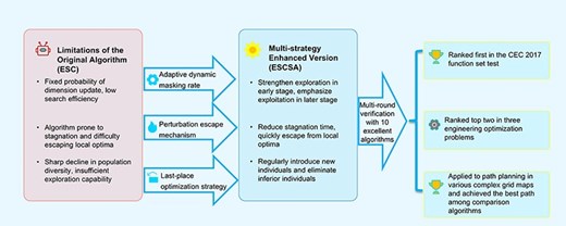
Dynamic mask adjustment balances exploration and exploitation.
The perturbation escape mechanism combined with Simulated Annealing enables quick escape from local optima.
Worst-elimination strategy maintains population diversity for more possibilities.
Ranked top two in the tests of CEC 2017 and three engineering optimization problems.
Applied to path planning and achieved the best path among comparison algorithms.
Nomenclature
- T
Maximum number of iterations
- |$Tem$|
Initial temperature of Simulated Annealing
- |$\alpha$|
Cooling coefficient of Simulated Annealing
- |$P( t )$|
Panic index in ESC algorithm
- E
Elite pool
- |${{x}_{i,j}}$|
Position of the ith agent in the jth dimension
- |${{x}_{n,j}}$|
jth dimension value of the neighborhood solution
- |${{f}_c}$|
Fitness of current solution
- |${{f}_n}$|
Fitness of neighborhood solution
- |$\Delta$|
Fitness difference between neighborhood and current solution
- P
Metropolis acceptance probability
- |$l{{b}_j}$|, |$u{{b}_j}$|
Lower and upper bound of the jth dimension
- N
Population size
- D
Problem dimension
- |$\beta$|
Adaptive parameter for Levy flight
- |${{w}_j}$|
Adaptive Levy weight
- |${{x}_{\textit{best}}}$|
Global optimal solution
1. Introduction
In the fields of science and engineering, numerous complex problems can be formulated as optimization problems, whose core is to find decision variables that maximize the objective function value under given constraints (Li et al., 2024). As problem complexity increases—such as through nonlinearity, high dimensionality, and multimodality—traditional deterministic optimization methods often face challenges due to their reliance on gradient information and susceptibility to local optima (Boussaïd et al., 2013; Fu et al., 2024). In this context, metaheuristic algorithms have gained widespread favor as efficient stochastic optimization techniques due to their independence from gradient information and robust global search capabilities (Fu et al., 2024; Mirjalili & Lewis, 2016).
The design of metaheuristic algorithms often draws inspiration from natural phenomena, physical laws, biological swarm intelligence, or human behavior. Their core principle is to balance exploration (i.e., broad global search) with exploitation (i.e., localized fine-grained search), guiding the population toward convergence on the global optimal solution (Wang et al., 2024). Based on their inspirational sources, metaheuristic algorithms can be broadly categorized as follows: Evolutionary-inspired algorithms center on the theory of biological evolution, achieving optimization by simulating natural selection, genetic mutation, and population iteration. For instance, Genetic Algorithms (GAs; Tuncer & Yildirim, 2012) draw on evolutionary principles, using selection, crossover, and mutation to drive populations toward optimal solutions. They find extensive applications in function optimization and combinatorial optimization. Differential Evolution (DE; Tuncer & Yildirim, 2012) employs differential vectors between population individuals for mutation, iteratively retaining superior individuals while eliminating inferior ones. It demonstrates excellent convergence speed and robustness in high-dimensional continuous optimization problems, making it particularly suited for scenarios such as engineering design parameter optimization. Swarm intelligence algorithms focus on the cooperative behavior of biological groups, enhancing search efficiency by simulating information exchange and collaboration mechanisms among individuals. For instance, Particle Swarm Optimization (PSO; Zhang et al., 2013) mimics bird foraging or fish schooling behavior, treating each solution as a “particle.” By tracking the optimal positions of the swarm and individual particles, it dynamically adjusts flight speed and direction, achieving mature applications in neural network training and path planning. Ant Colony Optimization (ACO; Tuncer & Yildirim, 2012) mimics how ants discover optimal foraging paths through pheromone trails and iteratively reinforce them via pheromone concentration updates to guide the colony toward optimal solutions. It excels at combinatorial optimization problems such as the traveling salesperson problem and vehicle routing. The Grey Wolf Optimizer (GWO; Mirjalili et al., 2014) simulates hierarchical leadership and prey-hunting strategies within wolf packs. By guiding the population search through alpha, beta, and delta wolves, it achieves global optimization, demonstrating strong global search capabilities in multimodal function optimization and engineering constraint problems. Algorithms based on physical and chemical laws construct optimization models grounded in intrinsic patterns of physical phenomena or chemical reactions, simulating energy changes and state transitions in natural processes. For instance, Simulated Annealing (SA; Kirkpatrick et al., 1983) draws on the physical principle that atoms gradually stabilize as temperature decreases during solid-state annealing. By gradually reducing the “temperature” parameter and accepting worse solutions with a certain probability, it effectively avoids getting stuck in local optima. It is widely applied in fields such as circuit design and image segmentation. Gravitational Search Algorithm (Rashedi et al., 2009) simulates the law of universal gravitation and Newton’s second law, treating individuals as “particles” with mass. Gravitational forces drive particles toward individuals with greater mass (higher fitness), demonstrating excellent search stability in multi-objective optimization and complex engineering problems. Algorithms inspired by human behavior draw insights from social activities and intelligent actions, mimicking human cognition and decision-making processes. For instance, Teaching-Learning-Based Optimization (Rao et al., 2011) simulates an interactive model in which a “teacher” guides “learners” to enhance knowledge during classroom instruction. By alternating between “teaching phases” and “learning phases,” it iteratively optimizes solution quality and is frequently applied in mechanical design optimization. The Hiking Optimization Algorithm (Oladejo et al., 2024) draws inspiration from human hiking movements. The Tobler Hiking Function accounts for the effects of terrain elevation and distance on hiking speed. By modeling the path-selection and speed-adjustment strategies of a “hiker,” it demonstrates superior solution accuracy and efficiency compared to traditional algorithms for NP-hard problems such as the Traveling Salesman Problem and the Knapsack Problem, as well as for engineering design optimization. Among diverse sources of inspiration, algorithms that mimic human intelligence and social behavior have emerged as a significant branch, thanks to their intuitive and effective approach, which offers a human-centric perspective for solving complex optimization problems.
It is worth noting that no single algorithm can achieve optimal performance across all problems. This core insight, revealed by the No Free Lunch Theorem (Li et al., 2024; Service, 2010), continues to drive the development of new algorithms and the refinement of existing ones. In recent years, metaheuristic algorithms inspired by novel natural phenomena and human behavior have emerged continuously, further enriching the research landscape in this field. For instance, the Hippopotamus Optimization (HO) algorithm (Amiri et al., 2024) simulates hippopotamus behavioral patterns, including position updates in rivers or ponds, defensive strategies against predators, and predator evasion tactics. The Puma Optimizer (Abdollahzadeh et al., 2024) models the hunting, pursuit, and escape mechanisms of pumas. The Parrot Optimizer (Lian et al., 2024) mimics the training behavior of Pyrrhura molinae parrots. The Secretary Bird Optimization Algorithm (Fu et al., 2024) simulates the hunting behavior of secretary birds and their evasion of predators. Beyond biologically or behaviorally inspired metaheuristics, recent years have witnessed the emergence of transformer-based optimization architectures as a complementary paradigm in computational intelligence. These methods leverage the attention mechanism originally developed for natural language processing to model complex dependencies in optimization problems. For instance, Schröder et al. systematically compared state-of-the-art reinforcement learning algorithms—including transformer-based architectures—applied to the TSP and the Orienteering Problem, finding that these methods can achieve near-optimal performance and generalize to larger problem sizes than those seen during training (Schröder et al., 2026). Abir et al. proposed GTG-ACO, a Graph Transformer Guided Ant Colony Optimization approach that jointly learns heuristic functions and initial pheromone matrices for combinatorial optimization problems. By augmenting Graph Transformers with Squeeze-and-Excitation networks, GTG-ACO dynamically captures structural relationships in graph representations and recalibrates feature importance, demonstrating improvements on problems such as the Traveling Salesman Problem (TSP) and Capacitated Vehicle Routing Problem (Abir et al., 2025). Although these transformer-based approaches often require substantial training data and computational resources, they represent an important emerging direction in optimization research. These novel algorithms offer innovative and efficient solutions to complex optimization problems by precisely modeling biological behaviors. However, single algorithms inevitably harbor inherent limitations. Over time, the constant emergence of new problems and the development of superior strategies have further exposed the inherent limitations of single algorithms (such as local optima, loss of population diversity, and insufficient convergence accuracy), rendering their optimization capabilities no longer a significant advantage (Boussaïd et al., 2013). To overcome these limitations, Hybrid Metaheuristic Algorithms have emerged. Hybrid strategies aim to integrate advantageous components from different algorithms or introduce novel strategies into existing metaheuristics, achieving complementary performance and synergistic enhancement (Faulin, 2012). Common hybridization approaches include: combining algorithms with strong global exploration capabilities with those possessing strong local exploitation capabilities; introducing adaptive mechanisms to adjust parameters or search strategies in an adaptive manner; or integrating techniques like Levy flight (Rocha et al., 2020), Opposition-Based Learning (Seif & Ahmadi, 2015; Yao et al., 2023), and the Nelder-Mead simplex method (Nelder & Mead, 1965) to enhance population initialization quality or local search efficiency. For instance, Zhang et al. proposed the MASSA hybrid algorithm, which combines circular chaotic mapping with Levy flight (Zhang et al., 2022). This approach incorporates Levy flight into the SSA optimization process and introduces a nonlinear inertia coefficient to balance global and local search capabilities. Mehta et al. proposed the Hybrid Mountain Gazelle Optimizer-Nelder-Mead, which combines the basic Mountain Gazelle Optimizer (MGO) with the Nelder-Mead simplex method. The MGO simulates MGO group formation, territory establishment, and foraging behavior. By integrating the global exploration of biological populations with the local, fine-grained search of the simplex method, this approach achieves statistically significant improvements over comparison algorithms in engineering optimization tasks (Mehta et al., 2024). Roman et al. applied the SMA to optimize parameters for Active Disturbance Rejection sliding mode control (ADRC-SMC). By leveraging the global optimization capability of metaheuristic algorithms, they enhanced real-time control performance in tower crane systems, validating the effectiveness of hybrid strategies in engineering control (Roman et al., 2024). The Artificial Lemming Algorithm (ALA), proposed by Xiao et al. provides a novel approach to solving engineering optimization problems by simulating the natural behaviors of lemmings, such as long-distance migration and burrowing, Subsequently, the team further combined Q-learning with an improved ALA, introducing an elite pool and a dynamic vertical crossover strategy, and achieved significant results in wind power generation forecasting (Xiao, Cui et al., 2025; Xiao et al., 2026). Furthermore, the MAROAOA algorithm demonstrated the potential of hybrid strategies in solving complex engineering problems by integrating arithmetic optimization with the artificial hare optimization algorithm (Xiao, Khurma et al., 2025). Research indicates that successful hybrid algorithms often exhibit superior performance in both CEC international benchmark tests and real-world engineering problems (Gao et al., 2026; Ghasemi et al., 2024; Mehta et al., 2024).
Path planning for mobile robots is a core problem in robotics that aims to autonomously determine safe, collision-free paths from a start to a goal position while minimizing travel distance and time in environments with static or dynamic obstacles (Contreras-Cruz et al., 2015; Mac et al., 2016). Path planning in static environments is termed global path planning, while that in dynamic environments is termed local path planning. As research has progressed, path planning studies have extended beyond autonomous driving to explore their engineering applicability in specific real-world scenarios. For example, Hu et al. proposed a LiDAR-camera fusion system for automated 3D crack detection, in which path planning for robotic arms is critical for close-range inspection (Hu et al., 2024). Ye et al. developed a bidirectional RRT* variant with kinematic constraints for orchard navigation, achieving significant improvements in path smoothness and computational efficiency (Ye et al., 2026). This problem is inherently complex, nonlinear, and typically classified as NP-hard (Yao et al., 2026). Traditional planning algorithms can be broadly classified into classical deterministic methods (e.g., Dijkstra, A*, Theta, D* Lite) and sampling-based methods (PRM, RRT, RRT*). Classical graph-search algorithms guarantee optimality and provide efficient solutions in static grid maps of low-to-medium complexity. A* in particular is widely recognized as the benchmark for structured environments due to its high success rate and low computational cost. However, their search space grows exponentially with map size and obstacle density, leading to excessive runtime and memory consumption in large-scale or high-dimensional problems. D* Lite supports dynamic replanning but still suffers from scalability issues in unknown or highly cluttered areas. Sampling-based methods such as RRT and PRM overcome certain dimensionality limitations and offer probabilistic completeness. RRT offers fast exploration, while RRT* improves path optimality at the cost of increased computation. Nevertheless, their path quality is inherently stochast they may produce jagged trajectories and require many iterations to converge, especially in environments with narrow corridors or dense obstacles (Ab Wahab et al., 2020; Almoaili & Kurdi, 2024; Faqas et al., 2025). At the same time, for multi–objective planning, these methods require additional mechanisms (e.g., scalarization or Pareto–based sampling), further increasing their computational burden (Yao et al., 2025).
Metaheuristic algorithms provide an effective approach for solving robot path planning in complex environments. These methods represent paths as sequences of waypoints or control points, indirectly optimizing overall path quality by adjusting the positions of these points (Shi et al., 2024; Zhang et al., 2023). Moreover, they naturally lend themselves to multi–objective optimization: a swarm can simultaneously evolve solutions that trade off path length, obstacle clearance, and energy consumption, either via Pareto ranking or through a dynamically weighted aggregate function. In recent years, various bio-inspired metaheuristic algorithms and their variants have been successfully applied to this problem. For example, Zhang et al. drew inspiration from the unique algorithmic design principles of radar technology to propose the wave search algorithm (Zhang et al., 2024). Applying this algorithm to six common engineering problems and robotic path planning yielded favorable results. Experimental results for static and dynamic path planning demonstrated significant advantages over the baseline algorithm. Garcia et al. proposed a novel approach based on the ACO algorithm (Garcia et al., 2009). In this approach, optimal path selection is based on criteria derived from a fuzzy reasoning system. Simultaneously, parameter adjustments via a simple tuning algorithm enable the robot to find optimal paths in both virtual simulations and real-world environments, significantly accelerating path planning speed. Ajeil et al. proposed a hybrid PSO-MFB algorithm (Ajeil et al., 2020) for path planning of autonomous mobile robots in static and dynamic environments. When the robot detects obstacles within its sensing range, the algorithm activates obstacle avoidance mechanisms to prevent collisions. Even in complex, dynamic environments, it generates optimal, feasible paths, effectively overcoming the shortcomings of traditional path-planning methods, such as grid-based approaches. Imen et al. combined the Improved Ant Colony Optimization (IACO) with GA to address global path planning for mobile robots in static environments (Châari et al., 2014), providing an effective solution for this scenario. Han et al., while exploring path planning for autonomous vehicles, proposed integrating ACO with GA (Heng & Rahiman, 2026), significantly improving shortest-path quality. These algorithms demonstrate considerable potential for handling complex constraints and finding high-quality paths, thanks to their robust global optimization capabilities.
Although existing metaheuristic algorithms offer diverse approaches to optimization problems, some still have room for improvement in balancing exploration and exploitation, robustness under complex constraints, and adaptability to specific scenarios (e.g., high-dimensional engineering optimization). In particular, the deep integration of human-behavior-based metaheuristic algorithms into engineering practice (e.g., robot path planning in complex environments) remains an area requiring further exploration in current research. The Escape algorithm (ESC) presents a novel optimization framework that simulates human evacuation behavior (Ouyang et al., 2024). It achieves the highest overall performance in comparisons with a total of 11 algorithms, including the Multi-Strategy Enhanced Gray Wolf Optimization (Ahmed et al., 2023), Gaussian Quantum Particle Swarm Optimization (Coelho, 2010), Improved Dung Beetle Optimizer (Y. H. Li et al., 2024), the Dominant Group Slime Mold Algorithm with Adaptive T-Distribution Mutation (Yin et al., 2022), Whale Optimization Algorithm (WOA; Mirjalili & Lewis, 2016), Crayfish Optimization Algorithm (COA; Jia et al., 2023), Sine Cosine Algorithm (Rizk-Allah & A. E. Hassanien, 2023), Spider Wasp Optimizer (SWO; Abdel-Basset et al., 2023), among others. However, it still has room for improvement in balancing exploration and exploitation, avoiding local optima, and maintaining population diversity. To address these limitations, this paper proposes a multi-strategy enhanced variant of the ESC—the ESCSA algorithm. The main contributions of this study include:
Designed a dynamic mask probability adjustment mechanism to achieve an adaptive balance between exploration and exploitation during the search process.
Introduced a local search strategy based on stagnation detection and SA (Kirkpatrick et al., 1983; Zhou et al., 2022) to enhance the algorithm’s ability to avoid local optima through refined local search.
Construct a worst-elimination strategy that periodically introduces new individuals at random positions while eliminating poor solutions, effectively maintaining population diversity and preventing premature convergence.
Using the CEC 2017 benchmark function and three engineering design problems—reduction gear design, multi-plate clutch braking, and rolling element bearing design—we comprehensively validated the performance and robustness of the ESCSA algorithm by comparing it with the original ESC algorithm and nine other algorithms.
Successfully applied the ESCSA algorithm to robot path planning problems in 40 × 40, 80 × 80, and 90 × 90 grid environments, demonstrating its global optimization capability under complex obstacle layouts and providing an efficient solution for mobile robot path planning.
The subsequent structure of this paper is as follows: Chapter 2 introduces the ESC; Chapter 3 introduces the multi-strategy enhanced ESC variant, termed the ESCSA algorithm, and comprehensively elaborates on the three enhancement strategies proposed in this study; Chapter 4 presents experimental analysis and results using the CEC 2017 benchmark functions; Chapter 5 focuses on engineering design optimization problems and robot path planning applications; Chapter 6 summarizes the entire paper and outlines future work.
2. Escape algorithm
The Escape algorithm (ESC) is a metaheuristic inspired by crowd emergency evacuation behavior (Ouyang et al., 2024). Its core principle involves simulating three typical behavioral groups during evacuation—calm, herding, and panic—to efficiently explore and exploit the solution space for complex optimization problems. This approach balances the algorithm’s global search capability with its local optimization ability. Specifically, the algorithm analogizes the solution space of an optimization problem to an evacuation scenario, search agents (individuals) to evacuees, and the optimal solution to a “safe exit.” By simulating crowd movement patterns under different behavioral modes—rational decision-making by calm individuals (guiding exploration direction), group following by herding individuals (enhancing local exploration), and random movement by panicked individuals (avoiding local optima)—the algorithm iteratively converges toward the optimal solution. The conceptual framework is illustrated in Figure 1, with the pseudocode for the original Escape algorithm provided in Algorithm 1.
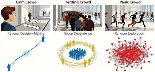
Conceptual diagram illustrating the Escape Algorithm inspired by simulating crowd evacuation behaviors.
Escape algorithm (ESC).
| 1: Initialize parameters and population |
| 2: Calculate initial fitness |${{f}_i} = f( {{{x}_i}} )$| |
| 3: Sort by fitness in ascending order |
| 4: Store the top existing individuals into the elite pool E |
| 5: Iterate t from 1 to T: |
| a: If t ≤ T/2 (exploration phase): |
| Divide populations proportionally into Calm, Follower, and Panic groups |
| Update positions for each group |
| b: If t > T/2 (Exploitation phase): |
| Update positions for all individuals |
| c: Recalculate fitness |$f_i^{new} = f( {x_i^{new}} )$| |
| d: Greedy selection: |${{x}_i} = x_i^{new}$| (if |$f_i^{new} \,\lt\, {{f}_i}$|), otherwise retain |${{x}_i}$| |
| e: Update the elite pool E as the current set of optimal individuals |
| 6: Output the optimal solution from the elite pool E |
2.1. Related definitions
Population: Composed of N search agents, each represented by a D-dimensional vector |${{x}_i} = ( {{{x}_{i,\ 1}},\ {{x}_{i,\ 2}},\ldots ,\ {{x}_{i,\ D}}} )$|, where |${{x}_{i,j}}$| denotes the position of the i-th agent in the j-th dimension, characterizing a potential solution to the optimization problem.
Elite Pool (E): Stores the highest-performing individuals in the population, symbolizing the “potential safe exits” identified by the crowd. It guides the search direction of other individuals. Defined as |$E = \{ {{{x}_{( 1 )}},{{x}_{( 2 )}},\ldots ,{{x}_{( {\textit{exist}} )}}} \}$|, where |${{x}_{( k )}}$| is the k-th optimal individual sorted in ascending order of fitness.
Panic Index (|$P( t )$|): An indicator reflecting the population’s overall “panic level,” gradually decreasing from 0 to the maximum iteration count T as the iteration count t progresses. This simulates the transition from chaos to adaptation during crowd evacuation and dynamically adjusts individual movement strategies, defined by Pt = cos (πt/6 T).
Exploration and Exploitation Phases: The boundary is set at iteration t < T/2. The first half constitutes the exploration phase (in which the population is divided into calm, herd-following, and panic groups, emphasizing global search). The second half constitutes the exploitation phase (all individuals in calm state, emphasizing local optimization).
2.2. Mathematical model
2.2.1. Population initialization
The initial position of each individual in the population is randomly generated within the feasible solution space using Equation 1:
where |$l{{b}_j}$| and |$u{{b}_j}$| denote the lower and upper bounds of the j-th dimension, respectively, and |${{r}_{i,j}}$| is a uniform random number in the interval [0,1], ensuring the randomness of the initial position distribution.
2.2.2. Exploration phase (|${\boldsymbol{t}} \le \frac{{\boldsymbol{T}}}{2}$|)
After sorting the population in ascending order of fitness, it is proportionally divided into a calm group (|$15\%$|), a herd group (|$35\%$|), and a panic group (|$50\%$|). Position update rules for each group are as follows:
Calm group update: Simulates rational decision-making by moving toward the group center, calculated as Equation 2:
where |${{C}_j}$| is the center of the calm group in dimension j (the mean of all calm individuals in that dimension), |${{v}_{c,j}} = {{R}_{c,j}} - {{x}_{i,j}} + {{\epsilon }_j}$| (|${{R}_{c,j}}$| is a random position within the calm group, |${{\epsilon }_j}$| is a fine-tuning term), and |${{m}_1}$| is a binary variable following a Bernoulli distribution (controls whether to update), |${{w}_1}$| is an adaptive Levy weight, calculated using a Levy distribution to simulate the step sizes in the exploration phase.
Conformist group update: Simulates following behavior influenced by both calm and panic groups, given by Equation 3:
where |${{x}_{p,j}}$| is a random individual in the panic group, |${{v}_{h,j}} = {{R}_{h,j}} - {{x}_{i,j}} + {{\epsilon }_j}$| (|${{R}_{h,j}}$| is a random position within the conformist group), |${{w}_2}$| is another adaptive Levy weight used for the conforming group, and |${{m}_2}$| is a binary variable which is generated through the same mechanism as |${{m}_1}$|.
Panic Group Update: Simulates random movement guided by the elite pool and random individuals in the population, given by Equation 4:
where |${{E}_j}$| is a random individual from the elite pool, |${{x}_{\text{rand},j}}$| is a random individual from the population, and |${{v}_{p,j}} = {{R}_{p,j}} - {{x}_{i,j}} + {{\epsilon }_j}$|(|${{R}_{p,j}}$| is a random position within the panic group).
2.2.3. Exploitation phase (|${\boldsymbol{t}} \ge \frac{{\boldsymbol{T}}}{2}$|)
All individuals undergo position refinement via calm behavior, moving toward the elite pool and random individuals to refine the solution. The formula is Equation 5:
where |${{E}_j}$| and |${{x}_{\text{rand},j}}$| represent the elite pool and a random individual in the population, respectively; |${{w}_1}$| and |${{w}_2}$| denote the adaptive Levy weights.
2.2.4. Adaptive Levy weights
Weight |${{w}_j}$| controls the movement step size of individuals, generated based on the Levy distribution, as given in Equation 6.
where |$\Gamma$| is the Gamma function, and |$\beta = {{\beta }_{\text{base}}} + 0.5 \times {\rm{sin}}( {\frac{{\pi t}}{{2T}}} )$| (|${{\beta }_{\text{base}}} = 1.5$|), enabling a dynamic transition from large-step exploration to small-step exploitation.
2.2.5. Elite pool update
After each iteration, the optimal solution is retained through greedy selection: if the fitness |$x_{i,j}^{\rm new}$| of the new position |$f_i^{\rm new}$| is less than |${{f}_i}$| (for minimization problems), the position is updated; otherwise, the original position is retained. The elite pool is simultaneously updated to the set of optimal individuals in the current population.
3. Improved Escape algorithm (ESCSA)
To address the limitations of the Escape algorithm in practical optimization problems—such as slow convergence, susceptibility to local optima, sharp decline in population diversity, and limited search capability—this paper proposes three enhancement strategies. These strategies are conceptual analogies or methodological heuristics, grounded in the ESC framework and general optimization principles. Figure 2 provides a simple and intuitive illustration of these improvement mechanisms and their effects. They are designed to be innovative yet lightweight, Table 1 shows a comparison with similar mechanisms described in other literature, as detailed below.
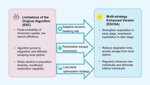
The principles of the ESCSA improvement mechanisms.
Comparison of ESCSA strategies with similar mechanisms reported in the literature.
| Strategy | Specific implementation in ESCSA | Typical working mechanism in the literature | Key differences |
|---|---|---|---|
| Dynamic mask probability adjustment | Stage-wise adjustment of the mask probability to control the proportion of dimensions updated. Fewer dimensions are updated in early iterations to accelerate discovery of promising regions (enhancing exploration), while more dimensions are updated in later iterations to improve local refinement (enhancing exploitation). | Adaptive tuning of key parameters according to the algorithm-specific framework to balance exploration and exploitation—e.g., modulating the convergence factor a in GWO to control the search range. | Tailored to ESC’s dimension-wise mask update rule, enabling precise control over which dimensions are updated at each stage. This provides finer-grained control compared with typical mechanisms that adjust overall search magnitude. |
| Stagnation-triggered SA | As an independent module triggered on demand using a relative stagnation threshold; performs systematic local search via SA to escape local optima. | Perturbation-based mechanisms are usually integrated into every iteration to enhance local search. | Combines on-demand triggering, scale-adaptive thresholding, and Gaussian perturbation synergy to address stagnation more specifically and systematically than per-iteration perturbation approaches. |
| Worst-elimination strategy | Merge-sort-truncate process: new individuals are merged with the current population, globally sorted, and the top N individuals are retained. | Diversity restoration via reinitialization of the entire population or random injection of individuals, often triggered by a diversity indicator. | Integrates elite preservation with a rank-based truncation mechanism, supported by parameter sensitivity analysis. This ensures that promising genetic material is never lost (maintaining convergence continuity), while global sorting guarantees that only high-quality new individuals are admitted (preventing performance degradation). In contrast, typical restart mechanisms lack such protection of elite information. |
A widely recognized core requirement in metaheuristic algorithms—balancing exploration and exploitation during the iterative process—motivates the dynamic adjustment of mask probability proposed in this study. However, there is no universal method for implementing this requirement; it must be customized to suit the specific characteristics of the algorithm’s framework. For example, PSO typically controls search behavior by adaptively adjusting the inertia weight (Kumar et al., 2020). In contrast, GWO modulates the search range via the convergence factor a (Nadimi-Shahraki et al., 2023). The proposed dynamic mask probability adjustment directly leverages the masking mechanism of the ESC. By dynamically adjusting the mask probability according to the iteration stage, it finely controls the exploration–exploitation balance at the dimensional level, thereby fully leveraging the structural feature of ESC—namely, its dimensional-level mask updates.
The local search enhancement mechanism customizes the integration of stagnation detection and SA for the ESC framework, manifesting at three levels. First, on-demand triggering: SA is activated only when the global optimum shows no significant improvement for |$T/25$| consecutive generations, thereby avoiding the high computational overhead of performing local search in every generation (Karaboga & Gorkemli, 2014; Yuan et al., 2025). Second, scale adaptability: a relative threshold (rather than an absolute one) is used to normalize fitness changes, ensuring that stagnation detection remains effective across objective functions of varying magnitudes. Third, Gaussian perturbation integration: Gaussian random perturbations are used to generate neighborhood solutions, which are then evaluated by the Metropolis rule to accept suboptimal solutions probabilistically, thus balancing local search precision with the ability to escape local optima. Together, these three elements constitute a lightweight yet effective local optimization scheme (Salgotra et al., 2021).
The worst-individual elimination strategy serves as a diversity preservation mechanism that incorporates three customized designs tailored to the ESC framework. First, a merge-sort-truncate mechanism: after new individuals are merged with the current population, the combined set is globally sorted and truncated; only those new individuals that outperform the current worst individual are allowed to enter the next generation, thereby preventing performance degradation caused by blind replacement. Second, elite preservation: global sorting ensures that elite individuals are never eliminated, maintaining the continuity of the convergence direction. Third, a fixed ratio aligned with the ESC iteration cycle: the injection interval of |$T/10$| and the number of injected individuals |$N/6$| have been validated through parameter sensitivity analysis (Tables 5 and 6). Within the 500-generation ESC framework, this configuration effectively replenishes diversity without disrupting the convergence trajectory of the main search. This fundamentally distinguishes the proposed strategy from common restart-based mechanisms.
3.1. Dynamic mask probability adjustment
In the original ESC algorithm, the mask probability—which controls the proportion of dimensions that remain unchanged during an update—was fixed (|${\rm{mask}}\_{\rm{probability}} = 0.5$|). A mask probability of 0.5 means each dimension has a 50% chance of remaining unchanged, helping to avoid excessive perturbation. The improved algorithm dynamically adjusts this probability according to the iteration stage, enabling a smooth transition from broad exploration to detailed exploitation. The dynamic adjustment mechanism works as follows:
Early iteration phase (0 to 1/3 T): A higher mask probability of 0.6 is used. Fewer dimensions participate in updates, preventing excessive disturbance, maintaining population stability, and emphasizing gradual exploration.
Mid-iteration phase (1/3 T to 2/3 T): The mask probability is set to 0.5 to balance global exploration and local exploitation. This maintains exploration of new regions while initiating refinement around high-quality solutions.
Late iteration phase (2/3 T to T): The mask probability is reduced to 0.4. More dimensions are updated, improving local search precision. This accelerates convergence toward the optimal solution by enhancing local optimization accuracy and emphasizing exploitation.
This dynamic adjustment enables the algorithm to precisely match search requirements at different stages, avoiding the challenge of balancing exploration and exploitation inherent in a fixed mask probability.
3.2. Stagnation detection and SA local search
To prevent the algorithm from getting stuck in local optima, an improved stagnation detection mechanism is introduced. When the optimal solution fails to improve for an extended period, the SA algorithm is triggered for localized refinement (Zhou et al., 2022). SA is based on modeling physical annealing processes. Its core principle is to introduce random perturbations and accept worse solutions with a certain probability, thereby efficiently searching for global optima (Kirkpatrick et al., 1983). Starting from an initial high-temperature state, the algorithm progressively reduces the acceptance probability of worse solutions as temperature decreases, ultimately converging near the global optimum.
3.2.1. Implementation details of the SA algorithm
Step 1: Parameter initialization: Set the initial temperature |$T{\rm{e}m} = 100$|, the cooling coefficient |$\alpha \ = \ 0.95$| (to control the temperature decay rate), and the maximum iteration count at each temperature |$\rm max\_iter = 100$|. Use the current solution (|${{x}_c}$|) as the initial solution and calculate its fitness (|${{f}_c}$|).
Step 2: Neighborhood solution generation: In each iteration, generate a neighborhood solution (|${{x}_n}$|) by introducing a Gaussian random perturbation, with Equation 7.
where |$\mathcal{N}( {0,1} )$| denotes a random number following a standard normal distribution, and 0.1 is the perturbation scale factor.
Step 3: Boundary control: To ensure solutions remain within the feasible region, dimensions exceeding upper/lower bounds are truncated using Equation 8:
where |$l{{b}_j}$| and |$u{{b}_j}$| denote the lower and upper bounds of dimension j, and |${{x}_{n,j}}$| is the value of the |$j - th$| dimension of the neighborhood solution |${{{\boldsymbol{x}}}_n}$|.
Step 4: Solution acceptance criteria: Calculate the fitness difference (|$\Delta = {{f}_n} - {{f}_c}$|) between the neighborhood solution’s fitness (|${{f}_n}$|) and the current solution’s fitness. If |$\Delta \,\lt\, 0$| (neighborhood solution is superior), directly accept the neighborhood solution; otherwise, accept it probabilistically using the Metropolis criterion, with Equation 9:
Here, P represents the Metropolis acceptance probability for inferior candidate solutions in the SA process. When the random number |${\rm rand} \sim U\ ( {0,1} )$| is less than P, accept the neighborhood solution; otherwise, retain the current solution.
Step 5: Temperature update: After each iteration, the temperature is linearly decayed according to Equation 10.
Step 6: Termination condition: When the maximum iteration count |$\rm max\_iter$| is reached, output the current optimal solution (|${{x}_{\textit{best}}}$|).
This algorithm transitions from “broad exploration” to “local refinement” by progressively decreasing the temperature: high temperatures permit the acceptance of worse solutions to avoid local optima, while low temperatures accept only better solutions to converge toward the global optimum, effectively complementing the local optimization capability of the ESC algorithm.
3.2.2. Specific strategy implementation
Stagnation detection condition: Let the current optimal fitness be |${{f}_{\text{best}}}$|, and the previous iteration’s optimal fitness be |$f_{\text{best}}^{\rm pre}$|. To ensure that the stagnation detection mechanism works consistently across test functions with varying objective magnitudes, we use a relative threshold instead of an absolute one. The stagnation condition is defined in Equation 11.
This relative criterion normalizes the fitness difference by the current best fitness value, making the threshold independent of the function’s scale. Consequently, the setting applies uniformly to low–magnitude functions (e.g., CEC 2017–F6 around 600) and high–magnitude functions (e.g., CEC 2017–F2 exceeding 1e100), eliminating the need for problem–specific tuning. When |$\rm {stagnatio{{n}_{\text{count}}} \ge \text{stagnatio}{{n}_{{\rm{threshold}}}}}$| (set as |$T/25$| in this paper, corresponding to 20), stagnation is detected. During stagnation, use the current best solution |${{x}_c}$| as the initial solution and execute SA optimization to generate a new solution |${{x}_{\rm new}}$|. If the new solution has a better fitness (|${{f}_{new}} \,\lt\, {{f}_{\textit{best}}}$|), update the population’s best solution by Equation 12:
Upon completing local search, if a better solution is found, update the population’s best solution and reset the stagnation counter. This ensures that the algorithm maintains convergence toward the global optimum. By employing the probabilistic acceptance criterion of SA, this mechanism helps the algorithm avoid local optima while systematically performing local search, thereby improving the precision of local exploration.
3.2.3. Worst-elimination strategy
As metaheuristic algorithms converge, population diversity rapidly diminishes. To maintain diversity, the worst-elimination strategy periodically introduces new individuals to replace poorer solutions within the population, preventing long-term iteration from causing population homogenization. Every |$T/10$| generations (corresponding to 50 generations in this paper), |$N/6$| new solutions (5 in this paper) are randomly generated and added to the population. These new solutions are uniformly distributed within the solution space as Equation 13:
Where |$k = 1,2,\ldots ,{\rm{\ }}M,j = 1,2,\ldots ,{\rm{\ }}{\rm dim},{\rm{and}}\ {{r}_{k,j}}$| is a uniform random number.
The expanded population is then sorted in ascending order of fitness. The N/6 least-fit individuals are eliminated, leaving the top N optimal solutions. This mechanism injects fresh vitality into the population, preventing the algorithm from losing its ability to explore new regions as diversity declines in later iterations. It is particularly suitable for complex optimization problems with high dimensions and multimodal characteristics, ensuring the algorithm maintains robust search vitality throughout the entire iteration process.
In summary, the improved algorithm dynamically balances exploration and exploitation by adjusting the mask probability, enhances local optimization accuracy through stagnation detection and SA, and maintains population diversity via the worst-elimination strategy. This significantly accelerates convergence, improves solution accuracy, and enhances performance for complex optimization problems. Figure 3 illustrates the detailed process diagram of the enhanced ESCSA algorithm. Below is the pseudocode for the Improved ESCSA algorithm in Algorithm 2.
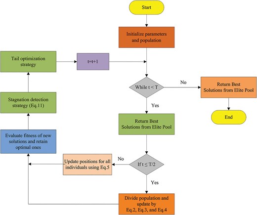
The detailed process diagram of ESCSA.
ESCSA algorithm.
| 1: Initialize parameters and population |
| 2: Evaluate fitness of each individual |${{f}_i} = f( {{{x}_i}} )$| |
| 3: Sort population by fitness in ascending order |
| 4: Store the top elite individuals in the Elite Pool: |$E = \{ {{{x}_{( 1 )}},{{x}_{( 2 )}},\ldots,{{x}_{( {\textit{exist}} )}}} \}$| |
| 5: Main Loop (Iterate t from 1 to T) |
| a: Adjust masking probability based on iteration progress: |
| If t ≤ T/3, masking probability = 0.6 |
| If T/3 < t ≤ 2T/3, masking probability = 0.5 |
| If t > 2T/3, masking probability = 0.4 |
| b: Update the solution position: |
| If t ≤ T/2 (exploration phase): |
| Divide population into: Calm group, Conforming group, and Panic group |
| Update Calm Group, Update Conforming Group, Update Panic Group |
| If t > T/2 (Exploitation phase): |
| Update positions for all individuals |
| c: Evaluate fitness of new solutions and retain optimal ones |
| d: Stagnation detection strategy |
| When |$\rm stagnatio{{n}_{\text{count}}}$| ≥ |$\rm stagnatio{{n}_{{\rm{threshold}}}}$|, execute Simulated Annealing optimization |
| Update the population’s optimal solution |
| Reset the |$\rm stagnatio{{n}_{\text{count}}}$| to 0 |
| e: Worst-elimination strategy |
| When |$t = k \cdot \frac{T}{{10}}$|, (|$k = 1,2,\ldots$|), generate N/6 new solutions randomly within the solution space to form a temporary expanded population |
| Compute the fitness of the expanded population and sort it in descending order |
| Retain the top N optimal solutions as the updated population |
| 6: Return Best Solutions from Elite Pool |
3.3. Complexity analysis of the ESCSA algorithm
The computational complexity analysis focuses on three key parameters: population size N, problem dimension D, and maximum iteration count T. The initialization phase and the main iteration loop primarily determine the computational complexity of ESCSA. The initialization phase includes population initialization, fitness evaluation, and sorting, with a complexity of |$O( {N \times D + N{\rm{log}}N} )$|. The main loop runs T iterations, each comprising the following operations: fitness sorting |$O( {N{\rm{log}}N} )$|, position update (including grouping operations, treated as |$O( {N \times D} )$|), boundary control |$O( {N \times D} )$|, fitness re-evaluation |$O( {N \times D} )$|), and population update and sorting |$O( {N{\rm{log}}N} )$|. Thus, the complexity of each iteration is |$O(N \times D + N{\rm{log}}N$|), and the overall complexity of the main loop is |$O( {T\ \times \ ( {N \times D + N{\rm{log}}N} )} )$|. Additionally, the ESCSA enhancement mechanism introduces additional overhead. SA local search is triggered when the optimal solution stagnates (at worst, triggered up to T/25 times). Each local search invocation runs 100 iterations of SA, with each iteration having a complexity of |$O( D )$|. Thus, the complexity per trigger is |$O( {100 \times D} )$|, which is negligible relative to the main loop. The worst-elimination strategy executes once every T/10 iteration, generating N/6 new individuals each time. It evaluates fitness and sorts the merged population, with a complexity of |$O( {N \times D + \textit{NlogN}} )$|. Thus, the total complexity is |$O( {T \times N \times D + T \times N{\rm{log}}N} )$|. However, since the main loop already encompasses these operations, the overall complexity remains dominated by it.
In summary, the overall computational complexity of ESCSA is |$O( {T \times N \times ( {D + \textit{logN}} )} )$|, which is identical to that of the original ESC algorithm. This indicates that although the enhancement mechanism introduces additional operations, it does not alter the asymptotic complexity trend, and the algorithm remains efficiently applicable to structured optimization problems. ESCSA enhances exploration and convergence through SA and worst-elimination strategies, making it suitable for scenarios demanding high precision while maintaining computational efficiency comparable to the original version.
Regarding memory overhead, the ESCSA algorithm stores a population of N individuals (each with D dimensions) and an elite pool containing |$\rm elite\_size$| individuals. For the highest dimension considered in this paper (|$D = 100$|, |$N = 30$|, |$\rm elite\_size = 5$|), the total memory occupied by the population and the elite pool is approximately |$( {30 + 5} ) \times 100 \times 8 = 28,000$| bytes (about 28 KB). The remaining auxiliary arrays (e.g., fitness values and sorting indices) require less than 1 KB, which is comparable to that of ESC, representing an extremely low memory footprint.
4. Experimental results and discussion
In this section, we evaluated ESCSA’s performance on the CEC 2017 benchmark suite (Wu et al., 2016). We conducted a convergence behavior analysis to validate ESCSA’s effectiveness and compared its numerical results with those of other leading algorithms. Furthermore, we used two nonparametric tests—the Wilcoxon rank-sum test and the Friedman rank-sum test—to assess the variance and overall performance of competing algorithms.
4.1. Benchmark functions
As part of the study, the CEC 2017 benchmark suite (Dim = 10, 30, 50, 100) comprising 30 test functions was used to evaluate the performance of the proposed ESCSA algorithm. The functions in this suite are categorized as follows: single-modal functions measure optimization speed and accuracy; multimodal types with multiple optima assess robustness; hybrid and composite functions test the algorithm’s ability to solve complex problems by combining characteristics of the former two. All experiments were conducted using MATLAB 2022a on a computer with an Intel Core i5-12400 CPU (2.50 GHz) with 16 GB RAM. The iteration count was set to 500, and the population size was 30. Detailed information regarding the CEC 2017 test suite is provided in Table 2.
Review the CEC 2017 test suite.
| Type | ID | Description | Dim | fmin |
|---|---|---|---|---|
| Unimodal | CEC 2017-F1 | Shifted and Rotated Bent Cigar Function | 10/30/50/100 | 100 |
| Unimodal | CEC 2017-F2 | Shifted and Rotated Sum of Different Power Function | 10/30/50/100 | 200 |
| Multimodal | CEC 2017-F3 | Shifted and Rotated Zakharov Function | 10/30/50/100 | 300 |
| Multimodal | CEC 2017-F4 | Shifted and Rotated Rosenbrock’s Function | 10/30/50/100 | 400 |
| Multimodal | CEC 2017-F5 | Shifted and Rotated Rastrigin’s Function | 10/30/50/100 | 500 |
| Multimodal | CEC 2017-F6 | Shifted and Rotated Expanded Scaffer’s F6 Function | 10/30/50/100 | 600 |
| Multimodal | CEC 2017-F7 | Shifted and Rotated Lunacek Bi_Rastrigin Function | 10/30/50/100 | 700 |
| Multimodal | CEC 2017-F8 | Shifted and Rotated Non—Continuous Rastrigin’s Function | 10/30/50/100 | 800 |
| Multimodal | CEC 2017-F9 | Shifted and Rotated Levy Function | 10/30/50/100 | 900 |
| Multimodal | CEC 2017-F10 | Shifted and Rotated Schwefel’s Function | 10/30/50/100 | 1000 |
| Hybrid | CEC 2017-F11 | Hybrid Function 1 (N = 3) | 10/30/50/100 | 1100 |
| Hybrid | CEC 2017-F12 | Hybrid Function 2 (N = 3) | 10/30/50/100 | 1200 |
| Hybrid | CEC 2017-F13 | Hybrid Function 3 (N = 3) | 10/30/50/100 | 1300 |
| Hybrid | CEC 2017-F14 | Hybrid Function 4 (N = 4) | 10/30/50/100 | 1400 |
| Hybrid | CEC 2017-F15 | Hybrid Function 5 (N = 4) | 10/30/50/100 | 1500 |
| Hybrid | CEC 2017-F16 | Hybrid Function 6 (N = 4) | 10/30/50/100 | 1600 |
| Hybrid | CEC 2017-F17 | Hybrid Function 6 (N = 5) | 10/30/50/100 | 1700 |
| Hybrid | CEC 2017-F18 | Hybrid Function 6 (N = 5) | 10/30/50/100 | 1800 |
| Hybrid | CEC 2017-F19 | Hybrid Function 6 (N = 5) | 10/30/50/100 | 1900 |
| Hybrid | CEC 2017-F20 | Hybrid Function 6 (N = 6) | 10/30/50/100 | 2000 |
| Composition | CEC 2017-F21 | Composition Function 1 (N = 5) | 10/30/50/100 | 2100 |
| Composition | CEC 2017-F22 | Composition Function 2 (N = 5) | 10/30/50/100 | 2200 |
| Composition | CEC 2017-F23 | Composition Function 3 (N = 5) | 10/30/50/100 | 2300 |
| Composition | CEC 2017-F24 | Composition Function 4 (N = 5) | 10/30/50/100 | 2400 |
| Composition | CEC 2017-F25 | Composition Function 5 (N = 3) | 10/30/50/100 | 2500 |
| Composition | CEC 2017-F26 | Composition Function 6 (N = 3) | 10/30/50/100 | 2600 |
| Composition | CEC 2017-F27 | Composition Function 7 (N = 5) | 10/30/50/100 | 2700 |
| Composition | CEC 2017-F28 | Composition Function 8 (N = 5) | 10/30/50/100 | 2800 |
| Composition | CEC 2017-F29 | Composition Function 9 (N = 5) | 10/30/50/100 | 2900 |
| Search range: [−100 100] | ||||
4.2. Analysis of ESCSA parameter selection
4.2.1. Dynamic mask probability parameter analysis
In Strategy 1, adjusting the mask probability to control the proportion of dimensional updates across different stages is an effective approach to further balance exploration and exploitation. The ESC algorithm uses a fixed mask probability of 0.5. In the early stage of the present study, preliminary tests were also conducted with different fixed values. However, the algorithm achieved optimal performance only when the mask probability was set to 0.5. Subsequently, the improved algorithm accounted for the fact that the first half of the ESC framework is the exploration phase and the second half is the exploitation phase. The entire search process was evenly divided into three stages, with the middle stage retaining a mask probability of 0.5 to serve as a transition. For the first and third stages, two numbers with an average of 0.5 were adopted, ensuring that the strategy does not increase computational resource requirements. Accordingly, experiments were conducted on different mask probability configurations for the three stages. The selected parameter sets and the corresponding results are shown in Table 3. As shown, when the mask probabilities for the three stages are set to 0.6, 0.5, and 0.4, respectively, the strategy achieves the most outstanding balance.
Dynamic mask probability parameter analysis.
| Parameter | 0.5 | 0.6, 0.5, 0.4 | 0.7, 0.5, 0.3 | 0.8, 0.5, 0.2 |
| Average rank | 2.37 | 2.27 | 2.57 | 2.63 |
| Rank | 2 | 1 | 3 | 4 |
Note: Bold values indicate the best average rank among all parameter combinations.
4.2.2. Stagnation detection threshold parameter analysis
The parameter settings of SA were adapted from the classical SA literature: the initial temperature was set sufficiently high to ensure broad exploration of the solution space in the early stage; the cooling coefficient was chosen within the empirically recommended range of 0.95–0.99 (Kirkpatrick et al., 1983; Hajek, 1988); and the perturbation scale (0.1) was calibrated to the normalized [0,1] decision space to balance local refinement and solution diversity. Specifically, the values |$\rm Tem = 100$|, |$\alpha = 0.95$|, and |$\rm max\_iter = 100$| were used for all experiments in this study. With these fixed parameters, SA serves as a local search strategy that not only enhances local exploitation in most problems discussed in this paper but also maintains an acceptable computational cost.
SA local search is triggered by a stagnation detection mechanism. A stagnation count threshold |${{K}_{\text{stag}}}$| was defined as the criterion for determining whether the algorithm has stagnated. When the number of consecutive iterations without significant improvement reaches this threshold, SA is activated to help escape local optima. To determine a reasonable value for |$\rm stagnatio{{n}_{\text{count}}}$|, six candidate thresholds (10, 20, 30, 40, 50, 60) were tested on seven representative functions (F1, F5, F10, F15, F20, F25, F30) from CEC 2017. Each parameter set was independently run 30 times, and the Friedman ranks of ESCSA on each function were computed. The results are summarized in Table 4.
Stagnation detection threshold parameter analysis.
| Threshold | F1 rank | F5 rank | F10 rank | F15 rank | F20 rank | F25 rank | F30 rank | Average rank |
|---|---|---|---|---|---|---|---|---|
| 10 | 5 | 1 | 6 | 1 | 4 | 2 | 1 | 2.857 |
| 20 | 4 | 3 | 1 | 2 | 2 | 1 | 2 | 2.143 |
| 30 | 2 | 4 | 3 | 3 | 1 | 4 | 3 | 2.857 |
| 40 | 3 | 6 | 5 | 4 | 3 | 6 | 5 | 4.571 |
| 50 | 1 | 5 | 2 | 5 | 5 | 3 | 4 | 3.571 |
| 60 | 6 | 2 | 4 | 6 | 6 | 5 | 6 | 5.000 |
Note: Bold values indicate the best average rank among all parameters.
As shown in Table 4, when the stagnation threshold was set to 20, the algorithm achieved the best average rank (2.143) across the seven functions, with the most balanced ranking across functions. A threshold that is too small (e.g., 10) triggers SA too early, interrupting the algorithm’s natural convergence process and thereby degrading the final solution quality. An excessively large threshold (e.g., 40, 50, or 60) significantly delays SA activation. This makes it difficult to escape local optima on multimodal functions, resulting in a marked decline in rank (average rank above 4.571). Therefore, |${{K}_{\text{stag}}} = 20$| (corresponding to 20 generations under a maximum iteration count |$T = 500$|) was selected as the stagnation detection threshold.
4.2.3. Worst-elimination strategy parameter analysis
The worst-elimination strategy involves two core parameters: the injection interval (how many generations between injections) and the number of individuals injected each time. A grid search was performed on these two parameters separately using the same seven CEC 2017 functions.
Injection interval: Fixing the number of injected individuals per injection at |$M = 5$|, intervals of 10, 30, 50, 70, 90, and 110 generations were tested. The results are shown in Table 5. When the injection interval was 50 generations, the algorithm achieved the best average rank (2.857). An excessively short interval (e.g., 10 generations) leads to frequent population perturbation, thereby disrupting the convergence trajectory. An overly long interval (e.g., 110 generations) provides insufficient diversity injection, leading to premature convergence. Therefore, the injection interval was set to 50 generations (i.e., |$T/10$|).
Worst-elimination strategy – injection interval analysis.
| Interval | F1 rank | F5 rank | F10 rank | F15 rank | F20 rank | F25 rank | F30 rank | Average rank |
|---|---|---|---|---|---|---|---|---|
| 10 | 2 | 3 | 1 | 6 | 5 | 3 | 6 | 3.714 |
| 30 | 6 | 4 | 3 | 3 | 6 | 4 | 5 | 4.429 |
| 50 | 3 | 2 | 2 | 2 | 2 | 5 | 4 | 2.857 |
| 70 | 4 | 6 | 4 | 1 | 4 | 1 | 2 | 3.143 |
| 90 | 1 | 5 | 6 | 4 | 1 | 6 | 1 | 3.429 |
| 110 | 5 | 1 | 5 | 5 | 3 | 2 | 3 | 3.429 |
Note: Bold values indicate the best average rank among all parameters.
Number of injected individuals: Fixing the injection interval at 50 generations, injections of 1, 3, 5, 7, 9, and 11 new individuals were tested (corresponding to proportions of approximately |$N/30$| to |$N/2.7$| for a population size |$N = 30$|). The results are shown in Table 6. Injecting 5 individuals (i.e., |$N/6$|) gave the best average rank (2.429), with rankings among the top for all functions. Injecting too few individuals (e.g., 1 or 3) provides limited diversity enhancement, causing the algorithm to stagnate on complex functions. Injecting too many individuals (e.g., 7, 9, 11) eliminates promising building blocks, disrupting the established convergence direction and reducing solution accuracy. Therefore, the number of individuals injected per cycle was set to |$M = N/6$|.
Worst-elimination strategy—number of injected individual analysis.
| Number | F1 rank | F5 rank | F10 rank | F15 rank | F20 rank | F25 rank | F30 rank | Average rank |
|---|---|---|---|---|---|---|---|---|
| 1 | 4 | 2 | 2 | 6 | 2 | 5 | 3 | 3.429 |
| 3 | 2 | 3 | 3 | 1 | 5 | 2 | 4 | 2.857 |
| 5 | 1 | 4 | 1 | 3 | 1 | 1 | 6 | 2.429 |
| 7 | 5 | 6 | 5 | 4 | 6 | 6 | 1 | 4.714 |
| 9 | 6 | 5 | 6 | 2 | 3 | 3 | 5 | 4.286 |
| 11 | 3 | 1 | 4 | 5 | 4 | 4 | 2 | 3.286 |
Note: Bold values indicate the best average rank among all parameters.
Based on the above experimental analyses, the core parameters of the ESCSA algorithm were determined as follows: the three-stage dynamic mask probabilities were set to (0.6, 0.5, 0.4); the stagnation detection threshold was set to 20 generations (i.e., |$T/25$|); the injection interval of the worst-elimination strategy was set to 50 generations (|$T/10$|), with 5 individuals injected each time (|$N/6$|). These parameters demonstrated excellent robustness and performance across the CEC 2017 benchmark suite, engineering optimization problems, and grid-based path planning tasks, providing parameter-level support for the overall superiority of the ESCSA algorithm.
4.3. Competitive algorithms
In this section, we evaluate ESCSA’s performance across multiple benchmark test suites. Advanced algorithms included in the comparison, besides the original Escape algorithm (ESC), comprise: WOA (Mirjalili & Lewis, 2016), COA (Jia et al., 2023), Harris Hawk Optimization Algorithm (HHO; Heidari et al., 2019), and Multi-Strategy Enhanced Gray Wolf Optimization (MELGWO) algorithm (Ahmed et al., 2023). Additionally, high-performance new algorithms published within the past year are included: Hippopotamus Optimization (HO) algorithm (Amiri et al., 2024), Fungal growth optimizer (FGO; Abdel-Basset et al., 2025), Horned Lizard Optimization Algorithm (HLGO; Peraza-Vázquez et al., 2024), Grey Geese Optimization Algorithm (GGO; El-kenawy et al., 2024), and Tribal Competition and Cooperation Optimization Algorithm (CTCM; Chen et al., 2025), totaling 10 comparison algorithms. In the experiments, the population size N for each algorithm was set to 30, and the maximum iteration count T was set to 500. All algorithms terminated upon reaching the maximum number of iterations (T = 500). Additionally, the parameters of each algorithm participating in the comparative test are shown in Table 7.
Parameter settings of the chosen algorithms.
| Algorithm | Parameters | Values |
|---|---|---|
| WOA | |$a1,\ a2,\ b$| | 2 to 0, (−1) to (−2), 1 |
| COA | |$C,\ \mu ,\ \sigma$| | 2 to (t/T), 25, 3 |
| HHO | |$E0,\ E1$| | [−1, 1], 2*(1 − (t/T) |
| MELGWO | |${\rm {Max}}_{\rm FE},\ {\rm Mi{{n}_{\text{Agent}{{s}_{no}}}}},\\{{F}_{\rm min}},\ {{F}_{\rm max}},pCR$| | 50 000, 10, 0.1, 2, 0.6 |
| HO | |${\rm Phase1}\_T\_{\rm threshold},\\\ \text{Levy}\_{\rm beta},\ b,\ c,\ d,\ l$| | [0.6, 1.5], [2,4], [1,1.5], [2, 4], [2, 3], [−2π, 2π] |
| FGO | |$M,\ Ep,\ R$| | 0.6, 0.7, 0.9 |
| HLOA | |${\rm Delta},\ Vo,\ c$| | 1 to 2, 1 to 10, 0.1 to 10 |
| GGO | |$a,\ c,\ b$| | 2 to 0, 2, 1 |
| CTCM | a | 2 to 0 |
| ESC | |$\beta \_{\rm base},\ \text{elite}\_{\rm Size},\\\ a,\ b,\text{mask}\_{\rm probability}$| | 1.5, 5, 0.15, 0.35, 0.5 |
| ESCSA | |$\beta \_{\rm base},\ \text{elite}\_{\rm Size},\\\ a,\ b,\text{mask}\_{\rm probability}$| | 1.5, 5, 0.15, 0.35, (0.6, 0.5, 0.4) |
In the performance comparison of metaheuristic algorithms, another common termination criterion is the maximum number of function evaluations (MaxFEs). To quantify the computational cost, the source code of each algorithm was analyzed line by line, with the average number of function evaluations (FEs) per iteration counted accordingly. The results are presented in Table 8. Here, N denotes the population size. For example, when N = 30, N evaluations correspond to 30 function calls. Due to the introduction of SA local search and the worst-elimination strategy, ESCSA incurs a small number of additional evaluations when these mechanisms are triggered (the SA local search is triggered infrequently, while the periodically triggered worst-elimination strategy adds approximately 0.003N evaluations per iteration on average). Overall, however, the number of evaluations per iteration remains approximately N. As shown in Table 8, all algorithms except HO, MELGWO, and HHO require approximately N evaluations per iteration.
Statistics on the number of evaluations per generation for the comparison algorithms in the experiment.
| Algorithm | HO, MELGWO | HHO | ESCSA and others |
|---|---|---|---|
| Evaluations per iteration (approx.) | 2.5N | 2N | N |
4.4. Ablation experiments
To verify the effectiveness and contribution of each improvement module in the proposed multi-strategy enhanced algorithm ESCSA, ablation experiments were conducted. Using the original ESC algorithm as the baseline, three improvement strategies were introduced: (1) dynamic mask probability adjustment (denoted as ESC_D), (2) stagnation detection with SA local search (denoted as ESC_S), and (3) worst-elimination strategy (denoted as ESC_W). The full ESCSA algorithm, which integrates all three strategies, was also retained. Accordingly, five variants were compared in the ablation study: ESC, ESC_D, ESC_S, ESC_W, and ESCSA. All variants were run under identical parameter settings (population size N = 30, maximum number of iterations T = 500, and 30 independent runs). As shown in Figure 4, all improved variants outperform the original ESC algorithm. Moreover, ESCSA achieves the best performance among the five variants across these subfigures. These results indicate that the three strategies are not only non-redundant but also synergistic, collectively contributing to ESCSA’s superior global optimization capability.
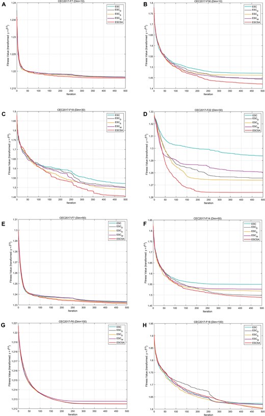
Performance of each sub-algorithm on the CEC 2017 function in the ablation experiments; subfigures (A–H) show their average convergence curves across four dimensions (10, 30, 50, and 100 dimensions).
The same conclusion can be drawn from Table 9, which summarizes the Friedman mean ranks of each variant on the CEC 2017 test suite across four dimensions (10, 30, 50, and 100). Across all dimensions, every enhanced variant outperforms the original ESC algorithm. Notably, in the 10-dimensional case, ESCSA ranks second, while ESC_S ranks first. This is expected, as ESC_S incorporates the local search enhancement strategy, which proves powerful across all dimensions and is particularly effective in low-dimensional settings. However, as the problem dimension increases from 10 to 30, 50, and 100, the test functions become substantially more challenging due to the exponential growth of the search space and the increasing complexity of the fitness landscape, which is characterized by more local optima and stronger variable interdependencies. Under these more demanding conditions, ESC_S alone no longer suffices; the full ESCSA, which additionally integrates dynamic mask probability adjustment and the worst-elimination strategy, achieves superior performance. Moreover, the Friedman mean rank gap between ESCSA and ESC_S widens notably from 30 to 50 dimensions, underscoring the advantages of the worst-elimination strategy in maintaining population diversity and the dynamic mask probability adjustment in balancing exploration and exploitation at medium to high dimensions (detailed in Sections 4.5.1 and 4.5.2, respectively).
Friedman mean rank test for CEC 2017 test suites.
| Dimensions algorithms | 10 | 30 | 50 | 100 | ||||
|---|---|---|---|---|---|---|---|---|
| Ave rank | Overall rank | Ave rank | Overall rank | Ave rank | Overall rank | Ave rank | Overall rank | |
| ESC | 3.667 | 5 | 3.767 | 5 | 3.767 | 5 | 3.933 | 5 |
| ESCSA | 2.500 | 2 | 2.000 | 1 | 1.567 | 1 | 1.733 | 1 |
| ESC_D | 3.433 | 3 | 3.333 | 3 | 3.333 | 3 | 2.833 | 3 |
| ESC_S | 1.933 | 1 | 2.533 | 2 | 2.867 | 2 | 2.800 | 2 |
| ESC_W | 3.467 | 4 | 3.433 | 4 | 3.467 | 4 | 3.667 | 4 |
Note: Bold values indicate the best average rank among all algorithms.
In summary, the three strategies—dynamic mask probability adjustment for adaptive exploration–exploitation balance, stagnation-triggered SA for local refinement, and worst-elimination for diversity preservation—work synergistically to enhance the global optimization capability and dimensional robustness of ESCSA across a wide range of problem complexities.
4.5. Quantitative analysis
4.5.1. Diversity experiment
To verify the effectiveness of the proposed multi-strategy enhanced ESCSA algorithm in maintaining population diversity, a comparative diversity experiment was conducted. The original ESC algorithm was used as the baseline and compared with the full ESCSA algorithm. Three representative functions from the CEC 2017 benchmark suite were selected: a unimodal function (F2), a multimodal function (F8), and a hybrid function (F14), all with dimensionality set to 30. All experiments used a population size of |$N = 30$| and a maximum number of iterations |$T = 500$|. Each algorithm was run independently 30 times on each function. Population diversity was measured using the normalized mean pairwise Euclidean distance (Nadimi-Shahraki & Zamani, 2022), as given in Equation 14:
where l and |${\boldsymbol{u}}$| are the lower and upper bound vectors of each dimension, respectively, and D is the problem dimension. The value of this metric lies in [0,1], with larger values indicating a more scattered distribution of individuals (stronger exploration ability).
For the three representative functions F2, F8, and F14, Figure 5 presents the convergence curves (left subplots, semi-logarithmic coordinates) and the population diversity curves (right subplots, linear coordinates) of ESC and ESCSA. The figures show that ESCSA maintains richer population diversity than ESC throughout nearly the entire search process. This occurs because each activation of the worst-elimination strategy may introduce promising new individuals, effectively replenishing the diversity lost due to selection pressure and enabling the algorithm to explore new feasible regions continuously.
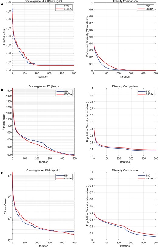
The first column shows the average fitness curves, and the second column shows the comparison of population diversity. Subfigures (A–C) illustrate a comparison of diversity across different types of functions.
4.5.2. Exploration and exploitation capability comparison experiment
To quantitatively analyze the global exploration and local exploitation behaviors of ESC and ESCSA during the iterative process, this section selects three representative functions from the CEC 2017 benchmark suite: a unimodal function (F2), a multimodal function (F8), and a hybrid function (F12). The evolution curves of exploration and exploitation ratios of ESC and ESCSA over iterations are compared. The experimental settings are as follows: population size = 30, maximum number of iterations = 500, dimension = 30. The curves are obtained by averaging over 30 independent runs to eliminate random fluctuations. The dimensional diversity index (Div(t)) method is adopted to compute the exploration and exploitation ratios at each generation, characterizing the evolution of the algorithm’s search pattern (Nadimi-Shahraki et al., 2023).
Let the population at generation t be denoted as |${{X}^t} = \{ {x_1^t,\ldots ,x_N^t} \}$| with dimension |$Dim$|. The dimensional diversity index is defined as Equation 15:
where |${{x}_{id}}( t )$| is the value of the ith individual in the dth dimension, and |${\rm{median}}( {{{x}_d}( t )} )$| is the median of that dimension. Based on |${\rm{Div}}( t )$|, the exploration and exploitation ratios are calculated as Equation 16:
where |${\rm{Di}}{{{\rm{v}}}_{{\rm{max}}}}$| is the maximum diversity index over the iteration process.
The experimental results are shown in Figure 6, where the red and blue curves represent the exploration and exploitation ratios, respectively; the solid lines correspond to ESCSA and the dashed lines to ESC. Both algorithms exhibit a typical “exploration-first, exploitation-later” transition pattern. In ESC, the exploration behavior decreases rapidly in the early stage. In contrast, the exploitation behavior increases sharply in the mid-to-late stage, which tends to trap the algorithm in local optima. In contrast, ESCSA integrates multiple strategies to achieve a smoother exploration–exploitation process, enabling a more thorough search of the solution space and thus a better balance between exploration and exploitation than the original ESC.
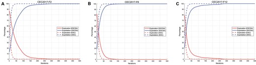
A comparison of the exploration and exploitation of the ESCSA algorithm and the original ESC algorithm. Subfigures (A–C) show comparisons across three types of functions.
4.5.3. Analysis of average convergence curves
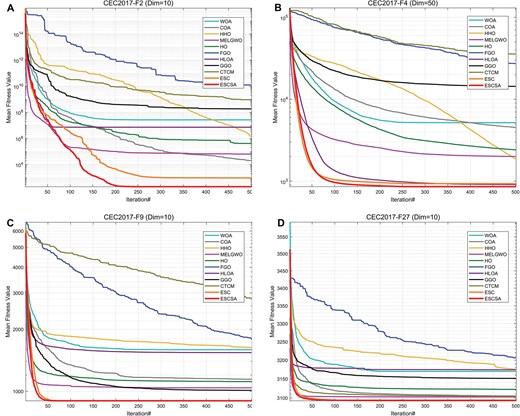
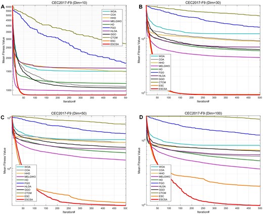
To provide a more intuitive comparison of optimization capabilities, Figures 7 –9 present the average convergence curves from 30 independent runs of ESCSA and the 10 comparison algorithms. Each figure views the curves from a different perspective. In terms of convergence accuracy, the ESCSA algorithm achieves superior values compared to other algorithms for most functions across various dimensions. ESC, HHO, MELGWO, and COA also demonstrate decent convergence accuracy, but none surpass ESCSA, as shown in Figure 7. In terms of convergence speed, ESCSA demonstrates outstanding performance and maintains adequate precision for most functions, as shown in Figure 8. For instance, in the 10-dimensional test of the F2 function, the ESCSA algorithm achieved rapid convergence before other high-precision algorithms had converged. In tests on the other three functions depicted, ESCSA converged near the optimal value within 50–100 iterations. When comparing convergence accuracy across different dimensions of the same test function, ESCSA showed particularly strong performance in high dimensions, as shown in Figure 9. The performance gap between ESCSA and ESC becomes increasingly pronounced as the dimensionality increases. The ESCSA algorithm builds upon the original ESC and dynamically adjusts the masking rate to balance exploration and exploitation better. It incorporates SA to boost local exploitation and adds a worst-elimination strategy. This strategy mitigates the typical decline in population diversity during iterations. It also enables the algorithm to avoid local optima and achieve higher convergence accuracy than the original ESC.
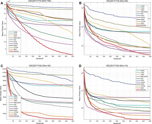
Convergence accuracy comparison chart (partial). Subfigures (A–D) illustrate the results for different representative functions.
Convergence speed comparison chart (partial). Subfigures (A–D) illustrate the results for different representative functions.
Performance comparison of 11 algorithms across different dimensions (using the F9 function as an analysis example). Subfigures (A–D) illustrate the results for different dimensions.
4.6. Quantitative evaluation
This section presents the comparative results between ESCSA and ten competing algorithms. The evaluation used the CEC 2017 benchmark suite across four dimensionalities: 10, 30, 50, and 100. The test results report the mean (Ave) and standard deviation (Std) for each of the 30 test functions, with each algorithm independently run 30 times. As shown in Tables 10–13, these tables correspond to the statistical outcomes of the 11 algorithms across the four dimensions. The optimal results for each metric in every row are highlighted in bold. Across both metrics in the four tables, ESCSA demonstrates outstanding performance across all dimensions of the CEC 2017 test suite. ESCSA secured the highest number of best values in both the mean and standard deviation metrics, highlighting ESCSA’s exceptional ability to handle complex, diverse functions.
Experimental results of 11 algorithms on the CEC 2017 (Dim = 10).
| ID | Index | WOA | COA | HHO | MELGWO | HO | FGO | HLOA | GGO | CTCM | ESC | ESCSA |
|---|---|---|---|---|---|---|---|---|---|---|---|---|
| F1 | Ave | 8.651E + 07 | 6.161E + 03 | 5.180E + 06 | 3.933E + 03 | 9.155E + 04 | 3.480E + 09 | 1.635E + 05 | 7.772E + 08 | 2.006E + 09 | 1.641E + 03 | 1.352E + 03 |
| Std | 1.147E + 08 | 4.598E + 03 | 1.952E + 07 | 4.935E + 03 | 2.471E + 05 | 1.229E + 09 | 6.180E + 05 | 1.084E + 09 | 6.535E + 08 | 2.279E + 03 | 1.696E + 03 | |
| F2 | Ave | 9.592E + 06 | 5.354E + 03 | 5.307E + 06 | 1.246E + 06 | 2.805E + 05 | 1.783E + 10 | 2.647E + 06 | 7.946E + 08 | 7.850E + 08 | 1.088E + 03 | 2.823E + 03 |
| Std | 1.845E + 07 | 2.117E + 04 | 8.851E + 06 | 6.547E + 06 | 5.996E + 05 | 5.389E + 10 | 1.220E + 07 | 3.164E + 09 | 7.511E + 08 | 1.610E + 03 | 3.527E + 03 | |
| F3 | Ave | 7.685E + 03 | 2.725E + 03 | 7.293E + 02 | 3.077E + 02 | 8.336E + 02 | 2.882E + 04 | 3.309E + 02 | 5.083E + 03 | 2.885E + 04 | 6.379E + 02 | 7.300E + 02 |
| Std | 6.827E + 03 | 2.008E + 03 | 3.828E + 02 | 1.126E + 01 | 3.865E + 02 | 1.127E + 04 | 3.569E + 01 | 2.353E + 03 | 7.206E + 03 | 4.307E + 02 | 5.566E + 02 | |
| F4 | Ave | 4.430E + 02 | 4.235E + 02 | 4.373E + 02 | 4.111E + 02 | 4.262E + 02 | 6.394E + 02 | 4.252E + 02 | 4.895E + 02 | 5.549E + 02 | 4.087E + 02 | 4.065E + 02 |
| Std | 5.150E + 01 | 2.844E + 01 | 4.450E + 01 | 1.784E + 01 | 3.130E + 01 | 1.050E + 02 | 3.058E + 01 | 6.986E + 01 | 4.435E + 01 | 1.344E + 01 | 6.198E-01 | |
| F5 | Ave | 5.575E + 02 | 5.355E + 02 | 5.626E + 02 | 5.249E + 02 | 5.455E + 02 | 5.827E + 02 | 5.683E + 02 | 5.338E + 02 | 5.692E + 02 | 5.066E + 02 | 5.067E + 02 |
| Std | 2.361E + 01 | 1.348E + 01 | 1.580E + 01 | 8.639E + 00 | 1.857E + 01 | 9.349E + 00 | 2.422E + 01 | 1.316E + 01 | 7.674E + 00 | 2.600E + 00 | 2.416E + 00 | |
| F6 | Ave | 6.366E + 02 | 6.093E + 02 | 6.380E + 02 | 6.092E + 02 | 6.273E + 02 | 6.418E + 02 | 6.481E + 02 | 6.130E + 02 | 6.404E + 02 | 6.000E + 02 | 6.000E + 02 |
| Std | 1.011E + 01 | 7.096E + 00 | 1.353E + 01 | 9.401E + 00 | 1.341E + 01 | 9.296E + 00 | 1.270E + 01 | 5.375E + 00 | 4.858E + 00 | 4.317E-05 | 3.281E-05 | |
| F7 | Ave | 7.875E + 02 | 7.844E + 02 | 7.873E + 02 | 7.434E + 02 | 7.637E + 02 | 8.401E + 02 | 7.982E + 02 | 7.562E + 02 | 9.048E + 02 | 7.203E + 02 | 7.181E + 02 |
| Std | 2.464E + 01 | 2.192E + 01 | 2.098E + 01 | 1.444E + 01 | 1.701E + 01 | 2.761E + 01 | 2.443E + 01 | 1.207E + 01 | 2.503E + 01 | 3.145E + 00 | 2.424E + 00 | |
| F8 | Ave | 8.494E + 02 | 8.339E + 02 | 8.339E + 02 | 8.198E + 02 | 8.245E + 02 | 8.790E + 02 | 8.413E + 02 | 8.287E + 02 | 8.810E + 02 | 8.069E + 02 | 8.068E + 02 |
| Std | 2.156E + 01 | 5.155E + 00 | 7.618E + 00 | 8.086E + 00 | 4.245E + 00 | 1.037E + 01 | 1.775E + 01 | 6.811E + 00 | 9.987E + 00 | 2.255E + 00 | 2.584E + 00 | |
| F9 | Ave | 1.488E + 03 | 1.078E + 03 | 1.442E + 03 | 1.034E + 03 | 1.184E + 03 | 1.858E + 03 | 1.645E + 03 | 1.000E + 03 | 2.616E + 03 | 9.000E + 02 | 9.000E + 02 |
| Std | 3.548E + 02 | 2.481E + 02 | 2.406E + 02 | 1.276E + 02 | 1.512E + 02 | 2.999E + 02 | 2.777E + 02 | 7.226E + 01 | 3.815E + 02 | 8.399E-02 | 1.407E-06 | |
| F10 | Ave | 2.154E + 03 | 2.394E + 03 | 2.143E + 03 | 1.844E + 03 | 1.873E + 03 | 2.964E + 03 | 2.452E + 03 | 2.200E + 03 | 2.328E + 03 | 1.483E + 03 | 1.306E + 03 |
| Std | 3.857E + 02 | 3.536E + 02 | 2.770E + 02 | 3.444E + 02 | 2.253E + 02 | 2.394E + 02 | 4.353E + 02 | 2.734E + 02 | 1.703E + 02 | 2.838E + 02 | 1.787E + 02 | |
| F11 | Ave | 1.240E + 03 | 1.134E + 03 | 1.181E + 03 | 1.162E + 03 | 1.175E + 03 | 2.004E + 03 | 1.210E + 03 | 1.239E + 03 | 1.532E + 03 | 1.104E + 03 | 1.103E + 03 |
| Std | 7.665E + 01 | 3.640E + 01 | 5.775E + 01 | 5.254E + 01 | 5.800E + 01 | 4.204E + 02 | 6.856E + 01 | 1.182E + 02 | 1.309E + 02 | 1.290E + 00 | 9.229E-01 | |
| F12 | Ave | 3.456E + 06 | 3.000E + 05 | 3.060E + 06 | 6.981E + 05 | 7.711E + 05 | 1.553E + 08 | 9.387E + 05 | 4.182E + 06 | 4.647E + 07 | 1.919E + 04 | 2.836E + 04 |
| Std | 4.075E + 06 | 8.981E + 05 | 2.974E + 06 | 6.169E + 05 | 1.333E + 06 | 7.980E + 07 | 1.967E + 06 | 4.605E + 06 | 1.817E + 07 | 1.881E + 04 | 5.936E + 04 | |
| F13 | Ave | 1.698E + 04 | 8.032E + 03 | 1.440E + 04 | 1.103E + 04 | 4.669E + 03 | 2.524E + 06 | 5.562E + 03 | 1.483E + 04 | 7.935E + 04 | 9.177E + 03 | 7.315E + 03 |
| Std | 1.150E + 04 | 6.434E + 03 | 1.187E + 04 | 8.975E + 03 | 2.080E + 03 | 2.418E + 06 | 5.256E + 03 | 8.996E + 03 | 6.613E + 04 | 7.606E + 03 | 6.444E + 03 | |
| F14 | Ave | 3.356E + 03 | 1.661E + 03 | 2.140E + 03 | 2.287E + 03 | 1.480E + 03 | 1.089E + 04 | 1.627E + 03 | 1.564E + 03 | 2.082E + 03 | 3.436E + 03 | 3.731E + 03 |
| Std | 1.572E + 03 | 1.536E + 02 | 9.542E + 02 | 1.178E + 03 | 2.024E + 01 | 9.810E + 03 | 1.820E + 02 | 7.441E + 01 | 5.124E + 02 | 3.317E + 03 | 3.143E + 03 | |
| F15 | Ave | 9.032E + 03 | 2.994E + 03 | 7.172E + 03 | 6.243E + 03 | 2.458E + 03 | 2.579E + 04 | 3.878E + 03 | 6.057E + 03 | 6.585E + 03 | 3.330E + 03 | 4.303E + 03 |
| Std | 6.289E + 03 | 1.938E + 03 | 3.291E + 03 | 4.258E + 03 | 7.963E + 02 | 2.900E + 04 | 5.926E + 03 | 3.326E + 03 | 2.617E + 03 | 2.942E + 03 | 3.786E + 03 | |
| F16 | Ave | 1.979E + 03 | 1.735E + 03 | 1.918E + 03 | 1.786E + 03 | 1.813E + 03 | 2.211E + 03 | 2.076E + 03 | 1.819E + 03 | 1.849E + 03 | 1.616E + 03 | 1.613E + 03 |
| Std | 1.855E + 02 | 1.170E + 02 | 1.416E + 02 | 1.538E + 02 | 1.319E + 02 | 1.230E + 02 | 2.039E + 02 | 1.072E + 02 | 7.242E + 01 | 3.077E + 01 | 2.479E + 01 | |
| F17 | Ave | 1.824E + 03 | 1.761E + 03 | 1.807E + 03 | 1.771E + 03 | 1.768E + 03 | 1.935E + 03 | 1.860E + 03 | 1.775E + 03 | 1.851E + 03 | 1.718E + 03 | 1.715E + 03 |
| Std | 6.760E + 01 | 2.143E + 01 | 6.733E + 01 | 4.819E + 01 | 1.339E + 01 | 7.001E + 01 | 1.361E + 02 | 2.383E + 01 | 3.642E + 01 | 1.478E + 01 | 2.336E + 01 | |
| F18 | Ave | 1.865E + 04 | 1.845E + 04 | 1.575E + 04 | 1.294E + 04 | 3.090E + 03 | 1.769E + 07 | 1.737E + 04 | 2.360E + 04 | 9.884E + 05 | 9.790E + 03 | 9.102E + 03 |
| Std | 1.233E + 04 | 1.289E + 04 | 1.338E + 04 | 1.014E + 04 | 3.874E + 03 | 1.664E + 07 | 1.514E + 04 | 1.694E + 04 | 9.904E + 05 | 6.230E + 03 | 6.841E + 03 | |
| F19 | Ave | 1.199E + 05 | 5.752E + 03 | 1.890E + 04 | 1.042E + 04 | 4.383E + 03 | 2.173E + 05 | 6.233E + 03 | 3.406E + 04 | 2.239E + 04 | 5.768E + 03 | 7.560E + 03 |
| Std | 2.965E + 05 | 7.941E + 03 | 1.943E + 04 | 7.701E + 03 | 3.576E + 03 | 2.822E + 05 | 7.289E + 03 | 6.823E + 04 | 1.743E + 04 | 6.818E + 03 | 7.379E + 03 | |
| F20 | Ave | 2.217E + 03 | 2.067E + 03 | 2.202E + 03 | 2.141E + 03 | 2.112E + 03 | 2.244E + 03 | 2.253E + 03 | 2.144E + 03 | 2.219E + 03 | 2.010E + 03 | 2.004E + 03 |
| Std | 8.655E + 01 | 4.021E + 01 | 7.039E + 01 | 7.213E + 01 | 5.509E + 01 | 6.372E + 01 | 9.991E + 01 | 6.137E + 01 | 5.411E + 01 | 2.251E + 01 | 8.798E + 00 | |
| F21 | Ave | 2.326E + 03 | 2.309E + 03 | 2.329E + 03 | 2.315E + 03 | 2.283E + 03 | 2.357E + 03 | 2.356E + 03 | 2.314E + 03 | 2.332E + 03 | 2.308E + 03 | 2.302E + 03 |
| Std | 5.875E + 01 | 5.046E + 01 | 4.929E + 01 | 4.032E + 01 | 6.355E + 01 | 3.337E + 01 | 4.771E + 01 | 3.782E + 01 | 5.275E + 01 | 1.911E + 01 | 2.472E + 01 | |
| F22 | Ave | 2.541E + 03 | 2.385E + 03 | 2.356E + 03 | 2.337E + 03 | 2.312E + 03 | 2.695E + 03 | 2.387E + 03 | 2.362E + 03 | 2.695E + 03 | 2.301E + 03 | 2.301E + 03 |
| Std | 5.270E + 02 | 3.682E + 02 | 2.259E + 02 | 1.849E + 02 | 6.656E + 00 | 1.735E + 02 | 2.955E + 02 | 6.289E + 01 | 1.391E + 02 | 4.300E-01 | 5.034E-01 | |
| F23 | Ave | 2.662E + 03 | 2.629E + 03 | 2.685E + 03 | 2.629E + 03 | 2.637E + 03 | 2.717E + 03 | 2.691E + 03 | 2.630E + 03 | 2.660E + 03 | 2.609E + 03 | 2.608E + 03 |
| Std | 2.492E + 01 | 1.267E + 01 | 3.498E + 01 | 1.273E + 01 | 1.470E + 01 | 3.922E + 01 | 4.998E + 01 | 1.174E + 01 | 5.098E + 00 | 2.869E + 00 | 2.009E + 00 | |
| F24 | Ave | 2.784E + 03 | 2.738E + 03 | 2.818E + 03 | 2.753E + 03 | 2.654E + 03 | 2.811E + 03 | 2.816E + 03 | 2.757E + 03 | 2.791E + 03 | 2.740E + 03 | 2.728E + 03 |
| Std | 3.818E + 01 | 7.981E + 01 | 1.083E + 02 | 9.044E + 00 | 1.141E + 02 | 6.192E + 01 | 7.851E + 01 | 2.827E + 01 | 7.090E + 00 | 3.776E + 00 | 3.388E + 01 | |
| F25 | Ave | 2.956E + 03 | 2.937E + 03 | 2.930E + 03 | 2.937E + 03 | 2.935E + 03 | 3.174E + 03 | 2.946E + 03 | 3.001E + 03 | 3.034E + 03 | 2.943E + 03 | 2.933E + 03 |
| Std | 5.983E + 01 | 6.915E + 01 | 2.426E + 01 | 3.284E + 01 | 2.392E + 01 | 1.313E + 02 | 3.184E + 01 | 5.969E + 01 | 2.347E + 01 | 1.509E + 01 | 2.187E + 01 | |
| F26 | Ave | 3.770E + 03 | 3.227E + 03 | 3.574E + 03 | 3.319E + 03 | 3.103E + 03 | 3.747E + 03 | 3.922E + 03 | 3.282E + 03 | 3.209E + 03 | 2.937E + 03 | 2.895E + 03 |
| Std | 5.536E + 02 | 5.342E + 02 | 5.261E + 02 | 4.841E + 02 | 3.696E + 02 | 2.231E + 02 | 6.086E + 02 | 3.464E + 02 | 4.597E + 01 | 1.680E + 02 | 6.186E + 01 | |
| F27 | Ave | 3.140E + 03 | 3.108E + 03 | 3.190E + 03 | 3.109E + 03 | 3.130E + 03 | 3.214E + 03 | 3.176E + 03 | 3.157E + 03 | 3.104E + 03 | 3.094E + 03 | 3.093E + 03 |
| Std | 4.161E + 01 | 2.016E + 01 | 5.040E + 01 | 2.770E + 01 | 4.945E + 01 | 3.775E + 01 | 7.485E + 01 | 4.932E + 01 | 1.920E + 00 | 3.598E + 00 | 2.590E + 00 | |
| F28 | Ave | 3.472E + 03 | 3.346E + 03 | 3.424E + 03 | 3.305E + 03 | 3.379E + 03 | 3.646E + 03 | 3.339E + 03 | 3.478E + 03 | 3.283E + 03 | 3.327E + 03 | 3.374E + 03 |
| Std | 1.414E + 02 | 1.409E + 02 | 1.870E + 02 | 1.212E + 02 | 9.781E + 01 | 1.136E + 02 | 1.557E + 02 | 1.861E + 02 | 1.877E + 01 | 1.153E + 02 | 8.309E + 01 | |
| F29 | Ave | 3.365E + 03 | 3.245E + 03 | 3.371E + 03 | 3.277E + 03 | 3.267E + 03 | 3.486E + 03 | 3.512E + 03 | 3.294E + 03 | 3.284E + 03 | 3.173E + 03 | 3.162E + 03 |
| Std | 1.256E + 02 | 5.849E + 01 | 9.116E + 01 | 7.724E + 01 | 6.334E + 01 | 1.146E + 02 | 2.014E + 02 | 7.986E + 01 | 4.101E + 01 | 1.962E + 01 | 1.562E + 01 | |
| F30 | Ave | 2.592E + 06 | 5.606E + 05 | 1.265E + 06 | 6.014E + 05 | 1.172E + 06 | 1.783E + 07 | 3.568E + 06 | 2.142E + 06 | 6.936E + 05 | 2.898E + 05 | 1.175E + 05 |
| Std | 3.542E + 06 | 6.319E + 05 | 1.679E + 06 | 1.005E + 06 | 1.160E + 06 | 9.682E + 06 | 6.942E + 06 | 2.859E + 06 | 2.316E + 05 | 3.591E + 05 | 2.461E + 05 |
Note: Bold indicates that the result is optimal.
To more intuitively illustrate the capabilities of different algorithms for solving optimization problems across various functions, Figure 10 compares the average Friedman rankings for each algorithm across 30 test functions in different dimensions (Kuyu & Vatansever, 2022). As shown in the figure, ESCSA maintains a leading position in the average rankings across all dimensions, particularly in high dimensions, demonstrating significantly superior performance compared to other algorithms. Table 14 summarizes the runtime data for each algorithm on the CEC 2017 test suite and ranks their performance based on Friedman’s test. Overall, ESCSA ranked first in the 10-, 30-, 50-, and 100-dimensional tests. This clearly demonstrates ESCSA’s leading capability in handling complex problems across multiple dimensions. Furthermore, to assess algorithmic stability, Figure 11 presents box plots comparing ESCSA with its competitors. ESCSA exhibits lower variance, indicating robust stability in problem-solving.
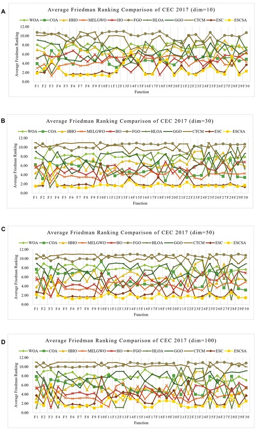
Average Friedman ranking of different algorithms on the CEC 2017 test suite. Subfigures (A–D) illustrate the results for different dimensions.
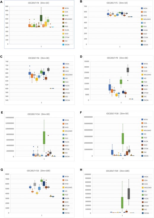
Boxplot comparison of different algorithms on the CEC 2017 test suite. Subfigures (A–H) illustrate the results for different representative functions.
While demonstrating formidable problem-handling capabilities in this evaluation, ESCSA also exhibits certain limitations. Its advantage diminishes in low-dimensional settings, particularly facing close competition from ESC. As the problem dimension increases, although ESCSA performs well on most functions, it underperforms other algorithms on a small number of functions. For example, in the 100-dimensional CEC 2017 tests, ESCSA does not achieve the best mean or standard deviation on functions F12, F13, and F25 (see Table 13). This indicates that the algorithm’s robustness can be further improved, representing a key direction for future enhancement.
4.7. Statistical analysis
4.7.1. Wilcoxon rank sum test
The Wilcoxon rank sum test is a nonparametric statistical method used to evaluate differences between ESCSA and its competing algorithms (Wilcoxon, 1992). The results, tested at a significance level of 5%, are presented in Table 15. The symbols “|$ +$|”, “|$ -$|”, and “|$ =$|” indicate that ESCSA performs better, worse, or as well as the comparison algorithm, respectively. The symbol “=” indicates no statistically significant difference between ESCSA and the compared algorithm. Considering the average values in Tables 10–13 alongside the Average Friedman ranking comparison in Figure 10, although ESCSA outperforms ESC on the vast majority of functions, the statistical results for ESC in the table reveal that, due to the lower complexity of low-dimensional problems, several high-performance algorithms can achieve satisfactory results—particularly advanced algorithms like ESC. Consequently, for a considerable number of functions in 10 and 30 dimensions, ESCSA’s advantage, while present, does not reach the threshold of statistical significance. As the dimensionality increases, ESCSA’s performance advantage becomes more pronounced, shifting from a “9/20/1” score at 10 dimensions to a “21/9/0” score at 100 dimensions. Compared with other algorithms, ESCSA demonstrates strong performance, achieving multiple “30/0/0” scores, particularly in high dimensions. In summary, the Wilcoxon rank-sum test results strongly validate the ESCSA algorithm’s outstanding performance across all dimensions of the CEC 2017 benchmark.
Experimental results of 11 algorithms on the CEC 2017(Dim = 30).
| ID | Index | WOA | COA | HHO | MELGWO | HO | FGO | HLOA | GGO | CTCM | ESC | ESCSA |
|---|---|---|---|---|---|---|---|---|---|---|---|---|
| F1 | Ave | 4.883E + 09 | 3.420E + 09 | 4.613E + 08 | 2.119E + 09 | 1.146E + 09 | 4.083E + 10 | 1.264E + 08 | 2.216E + 10 | 7.121E + 10 | 1.770E + 06 | 1.819E + 06 |
| Std | 1.708E + 09 | 3.969E + 09 | 3.743E + 08 | 1.847E + 09 | 8.963E + 08 | 4.955E + 09 | 4.963E + 07 | 7.073E + 09 | 6.262E + 09 | 9.314E + 06 | 8.791E + 06 | |
| F2 | Ave | 1.306E + 38 | 1.844E + 27 | 2.391E + 34 | 5.614E + 32 | 2.256E + 34 | 1.103E + 44 | 4.037E + 39 | 5.547E + 36 | 3.508E + 39 | 1.432E + 23 | 3.062E + 23 |
| Std | 7.148E + 38 | 5.396E + 27 | 7.683E + 34 | 2.888E + 33 | 1.083E + 35 | 5.183E + 44 | 2.210E + 40 | 1.575E + 37 | 8.407E + 39 | 7.115E + 23 | 9.962E + 23 | |
| F3 | Ave | 2.901E + 05 | 1.084E + 05 | 5.628E + 04 | 4.831E + 04 | 6.033E + 04 | 2.700E + 05 | 3.429E + 04 | 9.473E + 04 | 2.728E + 05 | 9.868E + 04 | 9.404E + 04 |
| Std | 7.600E + 04 | 3.241E + 04 | 6.870E + 03 | 9.067E + 03 | 7.851E + 03 | 2.205E + 05 | 1.010E + 04 | 1.530E + 04 | 4.047E + 04 | 2.243E + 04 | 1.958E + 04 | |
| F4 | Ave | 1.369E + 03 | 7.922E + 02 | 7.027E + 02 | 6.774E + 02 | 7.303E + 02 | 9.493E + 03 | 6.032E + 02 | 3.572E + 03 | 9.603E + 03 | 5.216E + 02 | 5.318E + 02 |
| Std | 3.605E + 02 | 2.466E + 02 | 9.190E + 01 | 1.648E + 02 | 1.301E + 02 | 2.856E + 03 | 6.055E + 01 | 1.367E + 03 | 1.927E + 03 | 2.768E + 01 | 2.697E + 01 | |
| F5 | Ave | 8.407E + 02 | 7.775E + 02 | 7.637E + 02 | 6.949E + 02 | 7.365E + 02 | 9.154E + 02 | 8.044E + 02 | 7.777E + 02 | 9.846E + 02 | 6.023E + 02 | 5.888E + 02 |
| Std | 4.975E + 01 | 6.867E + 01 | 3.168E + 01 | 4.535E + 01 | 4.218E + 01 | 3.282E + 01 | 4.962E + 01 | 3.550E + 01 | 2.972E + 01 | 2.037E + 01 | 1.346E + 01 | |
| F6 | Ave | 6.787E + 02 | 6.645E + 02 | 6.694E + 02 | 6.490E + 02 | 6.623E + 02 | 6.850E + 02 | 6.775E + 02 | 6.538E + 02 | 6.986E + 02 | 6.001E + 02 | 6.001E + 02 |
| Std | 1.264E + 01 | 1.326E + 01 | 6.201E + 00 | 8.704E + 00 | 7.348E + 00 | 8.865E + 00 | 1.257E + 01 | 7.560E + 00 | 7.342E + 00 | 2.691E-01 | 2.652E-01 | |
| F7 | Ave | 1.322E + 03 | 1.217E + 03 | 1.330E + 03 | 1.037E + 03 | 1.144E + 03 | 1.725E + 03 | 1.343E + 03 | 1.169E + 03 | 3.346E + 03 | 8.535E + 02 | 8.318E + 02 |
| Std | 9.192E + 01 | 1.169E + 02 | 7.266E + 01 | 7.205E + 01 | 6.855E + 01 | 1.223E + 02 | 7.121E + 01 | 7.431E + 01 | 2.119E + 02 | 1.458E + 01 | 1.641E + 01 | |
| F8 | Ave | 1.081E + 03 | 1.023E + 03 | 9.890E + 02 | 9.523E + 02 | 9.573E + 02 | 1.182E + 03 | 1.021E + 03 | 1.026E + 03 | 1.269E + 03 | 9.080E + 02 | 8.840E + 02 |
| Std | 5.057E + 01 | 2.081E + 01 | 1.910E + 01 | 2.536E + 01 | 2.345E + 01 | 2.675E + 01 | 3.838E + 01 | 2.537E + 01 | 2.399E + 01 | 1.754E + 01 | 1.591E + 01 | |
| F9 | Ave | 1.123E + 04 | 8.366E + 03 | 8.668E + 03 | 4.537E + 03 | 5.987E + 03 | 1.635E + 04 | 7.014E + 03 | 6.323E + 03 | 2.719E + 04 | 9.309E + 02 | 9.157E + 02 |
| Std | 3.479E + 03 | 2.271E + 03 | 1.033E + 03 | 1.070E + 03 | 9.684E + 02 | 2.594E + 03 | 9.679E + 02 | 1.295E + 03 | 2.921E + 03 | 5.084E + 01 | 2.075E + 01 | |
| F10 | Ave | 7.442E + 03 | 7.031E + 03 | 6.214E + 03 | 5.425E + 03 | 5.494E + 03 | 9.776E + 03 | 6.689E + 03 | 8.268E + 03 | 8.689E + 03 | 7.090E + 03 | 5.161E + 03 |
| Std | 9.550E + 02 | 1.233E + 03 | 7.262E + 02 | 7.930E + 02 | 5.834E + 02 | 2.930E + 02 | 7.841E + 02 | 4.915E + 02 | 3.783E + 02 | 5.725E + 02 | 5.184E + 02 | |
| F11 | Ave | 9.943E + 03 | 2.024E + 03 | 1.604E + 03 | 1.708E + 03 | 1.881E + 03 | 1.738E + 04 | 1.451E + 03 | 8.529E + 03 | 1.623E + 04 | 1.296E + 03 | 1.274E + 03 |
| Std | 4.540E + 03 | 8.785E + 02 | 1.673E + 02 | 6.425E + 02 | 3.234E + 02 | 5.077E + 03 | 7.435E + 01 | 2.647E + 03 | 3.204E + 03 | 1.363E + 02 | 5.971E + 01 | |
| F12 | Ave | 4.712E + 08 | 2.093E + 07 | 1.015E + 08 | 6.496E + 07 | 1.254E + 08 | 5.972E + 09 | 3.144E + 07 | 1.558E + 09 | 5.447E + 09 | 2.359E + 06 | 1.997E + 06 |
| Std | 3.307E + 08 | 2.145E + 07 | 1.288E + 08 | 9.000E + 07 | 1.240E + 08 | 1.529E + 09 | 2.886E + 07 | 1.241E + 09 | 9.583E + 08 | 1.791E + 06 | 1.590E + 06 | |
| F13 | Ave | 8.349E + 06 | 1.566E + 05 | 1.750E + 06 | 1.061E + 05 | 1.689E + 05 | 2.818E + 09 | 8.230E + 05 | 1.487E + 08 | 1.957E + 09 | 1.657E + 04 | 1.684E + 04 |
| Std | 6.238E + 06 | 2.013E + 05 | 4.111E + 06 | 8.711E + 04 | 2.387E + 05 | 1.490E + 09 | 1.659E + 06 | 3.016E + 08 | 5.605E + 08 | 1.118E + 04 | 1.021E + 04 | |
| F14 | Ave | 2.373E + 06 | 3.502E + 05 | 1.109E + 06 | 3.434E + 05 | 4.388E + 05 | 7.425E + 06 | 2.258E + 05 | 1.987E + 06 | 1.713E + 06 | 1.940E + 05 | 1.712E + 05 |
| Std | 2.397E + 06 | 4.442E + 05 | 8.708E + 05 | 4.178E + 05 | 4.485E + 05 | 4.281E + 06 | 3.159E + 05 | 2.236E + 06 | 1.086E + 06 | 2.277E + 05 | 3.102E + 05 | |
| F15 | Ave | 6.478E + 06 | 3.650E + 04 | 1.069E + 05 | 3.378E + 04 | 4.550E + 04 | 5.755E + 08 | 3.015E + 07 | 3.442E + 07 | 1.522E + 08 | 9.601E + 03 | 9.536E + 03 |
| Std | 1.138E + 07 | 3.313E + 04 | 6.008E + 04 | 2.214E + 04 | 3.167E + 04 | 3.224E + 08 | 1.649E + 08 | 6.926E + 07 | 8.042E + 07 | 8.497E + 03 | 8.382E + 03 | |
| F16 | Ave | 4.315E + 03 | 3.233E + 03 | 3.742E + 03 | 3.006E + 03 | 3.684E + 03 | 5.330E + 03 | 4.450E + 03 | 3.593E + 03 | 4.536E + 03 | 2.396E + 03 | 2.236E + 03 |
| Std | 6.884E + 02 | 3.951E + 02 | 4.812E + 02 | 3.098E + 02 | 5.569E + 02 | 4.016E + 02 | 1.111E + 03 | 3.009E + 02 | 2.465E + 02 | 1.900E + 02 | 2.377E + 02 | |
| F17 | Ave | 2.734E + 03 | 2.431E + 03 | 2.573E + 03 | 2.395E + 03 | 2.436E + 03 | 3.477E + 03 | 3.045E + 03 | 2.535E + 03 | 3.142E + 03 | 1.915E + 03 | 1.874E + 03 |
| Std | 3.426E + 02 | 2.414E + 02 | 2.197E + 02 | 2.121E + 02 | 2.709E + 02 | 2.246E + 02 | 3.333E + 02 | 2.654E + 02 | 1.585E + 02 | 1.325E + 02 | 9.841E + 01 | |
| F18 | Ave | 2.331E + 07 | 2.762E + 06 | 2.321E + 06 | 1.156E + 06 | 1.254E + 06 | 7.338E + 07 | 1.552E + 06 | 1.290E + 07 | 2.171E + 07 | 7.659E + 05 | 3.658E + 05 |
| Std | 2.892E + 07 | 1.915E + 06 | 2.405E + 06 | 1.507E + 06 | 1.557E + 06 | 4.449E + 07 | 1.870E + 06 | 2.034E + 07 | 1.099E + 07 | 8.696E + 05 | 3.657E + 05 | |
| F19 | Ave | 2.188E + 07 | 1.825E + 04 | 1.769E + 06 | 1.411E + 05 | 2.855E + 06 | 5.811E + 08 | 2.339E + 05 | 6.710E + 07 | 2.912E + 08 | 1.013E + 04 | 1.112E + 04 |
| Std | 1.929E + 07 | 1.969E + 04 | 1.811E + 06 | 2.200E + 05 | 1.721E + 06 | 2.464E + 08 | 3.385E + 05 | 1.403E + 08 | 1.142E + 08 | 1.099E + 04 | 1.244E + 04 | |
| F20 | Ave | 2.903E + 03 | 2.840E + 03 | 2.831E + 03 | 2.712E + 03 | 2.621E + 03 | 3.380E + 03 | 3.046E + 03 | 2.769E + 03 | 3.148E + 03 | 2.247E + 03 | 2.250E + 03 |
| Std | 2.007E + 02 | 2.088E + 02 | 2.300E + 02 | 2.598E + 02 | 1.149E + 02 | 1.523E + 02 | 2.530E + 02 | 1.688E + 02 | 1.335E + 02 | 1.190E + 02 | 1.238E + 02 | |
| F21 | Ave | 2.646E + 03 | 2.517E + 03 | 2.607E + 03 | 2.466E + 03 | 2.548E + 03 | 2.695E + 03 | 2.656E + 03 | 2.547E + 03 | 2.751E + 03 | 2.399E + 03 | 2.394E + 03 |
| Std | 7.362E + 01 | 4.461E + 01 | 6.373E + 01 | 3.485E + 01 | 4.442E + 01 | 3.369E + 01 | 7.768E + 01 | 3.398E + 01 | 2.459E + 01 | 2.420E + 01 | 1.523E + 01 | |
| F22 | Ave | 8.418E + 03 | 3.929E + 03 | 7.202E + 03 | 6.258E + 03 | 5.804E + 03 | 8.878E + 03 | 7.909E + 03 | 5.321E + 03 | 1.030E + 04 | 4.833E + 03 | 3.361E + 03 |
| Std | 1.613E + 03 | 1.789E + 03 | 1.422E + 03 | 1.631E + 03 | 2.093E + 03 | 1.637E + 03 | 1.459E + 03 | 1.137E + 03 | 2.337E + 02 | 3.149E + 03 | 1.786E + 03 | |
| F23 | Ave | 3.143E + 03 | 2.894E + 03 | 3.300E + 03 | 2.854E + 03 | 3.013E + 03 | 3.396E + 03 | 3.428E + 03 | 3.045E + 03 | 3.122E + 03 | 2.743E + 03 | 2.737E + 03 |
| Std | 9.301E + 01 | 5.395E + 01 | 1.385E + 02 | 5.695E + 01 | 8.917E + 01 | 9.339E + 01 | 1.718E + 02 | 7.177E + 01 | 3.557E + 01 | 3.104E + 01 | 1.849E + 01 | |
| F24 | Ave | 3.310E + 03 | 3.062E + 03 | 3.498E + 03 | 2.992E + 03 | 3.247E + 03 | 3.621E + 03 | 3.572E + 03 | 3.214E + 03 | 3.223E + 03 | 2.935E + 03 | 2.925E + 03 |
| Std | 1.159E + 02 | 4.971E + 01 | 1.629E + 02 | 4.231E + 01 | 8.676E + 01 | 9.617E + 01 | 2.125E + 02 | 8.423E + 01 | 3.255E + 01 | 2.272E + 01 | 1.489E + 01 | |
| F25 | Ave | 3.206E + 03 | 3.236E + 03 | 3.017E + 03 | 3.006E + 03 | 3.048E + 03 | 5.275E + 03 | 2.994E + 03 | 3.530E + 03 | 9.827E + 03 | 2.930E + 03 | 2.926E + 03 |
| Std | 6.651E + 01 | 1.580E + 02 | 4.045E + 01 | 5.628E + 01 | 3.582E + 01 | 8.211E + 02 | 4.282E + 01 | 2.110E + 02 | 1.450E + 03 | 3.191E + 01 | 2.523E + 01 | |
| F26 | Ave | 8.686E + 03 | 6.581E + 03 | 8.445E + 03 | 6.395E + 03 | 6.925E + 03 | 1.068E + 04 | 9.547E + 03 | 7.032E + 03 | 9.017E + 03 | 4.392E + 03 | 4.283E + 03 |
| Std | 1.001E + 03 | 1.419E + 03 | 7.360E + 02 | 8.705E + 02 | 1.262E + 03 | 6.780E + 02 | 1.346E + 03 | 5.741E + 02 | 4.203E + 02 | 2.381E + 02 | 3.585E + 02 | |
| F27 | Ave | 3.491E + 03 | 3.320E + 03 | 3.753E + 03 | 3.357E + 03 | 3.481E + 03 | 4.145E + 03 | 3.604E + 03 | 3.640E + 03 | 3.442E + 03 | 3.232E + 03 | 3.224E + 03 |
| Std | 1.579E + 02 | 3.735E + 01 | 3.300E + 02 | 9.088E + 01 | 1.184E + 02 | 1.447E + 02 | 2.842E + 02 | 2.141E + 02 | 3.545E + 01 | 1.334E + 01 | 7.415E + 00 | |
| F28 | Ave | 3.979E + 03 | 3.748E + 03 | 3.480E + 03 | 3.433E + 03 | 3.458E + 03 | 6.477E + 03 | 3.353E + 03 | 4.928E + 03 | 6.409E + 03 | 3.332E + 03 | 3.324E + 03 |
| Std | 6.682E + 02 | 2.159E + 02 | 6.405E + 01 | 1.068E + 02 | 7.792E + 01 | 5.415E + 02 | 3.615E + 01 | 4.261E + 02 | 8.382E + 02 | 3.637E + 01 | 4.121E + 01 | |
| F29 | Ave | 5.350E + 03 | 4.317E + 03 | 5.027E + 03 | 4.466E + 03 | 5.092E + 03 | 6.589E + 03 | 6.240E + 03 | 4.932E + 03 | 5.228E + 03 | 3.621E + 03 | 3.601E + 03 |
| Std | 5.504E + 02 | 3.084E + 02 | 3.644E + 02 | 3.579E + 02 | 4.596E + 02 | 5.292E + 02 | 7.178E + 02 | 4.586E + 02 | 1.806E + 02 | 1.326E + 02 | 8.633E + 01 | |
| F30 | Ave | 6.047E + 07 | 1.598E + 06 | 2.406E + 07 | 3.303E + 06 | 2.497E + 07 | 4.764E + 08 | 8.699E + 06 | 1.379E + 08 | 3.275E + 08 | 3.152E + 04 | 5.231E + 04 |
| Std | 5.361E + 07 | 2.613E + 06 | 6.071E + 07 | 2.464E + 06 | 2.145E + 07 | 1.785E + 08 | 9.882E + 06 | 1.220E + 08 | 1.095E + 08 | 2.910E + 04 | 4.869E + 04 |
Note: Bold indicates that the result is optimal.
Experimental results of 11 algorithms on the CEC 2017 (Dim = 50).
| ID | Index | WOA | COA | HHO | MELGWO | HO | FGO | HLOA | GGO | CTCM | ESC | ESCSA |
|---|---|---|---|---|---|---|---|---|---|---|---|---|
| F1 | Ave | 1.971E + 10 | 2.824E + 10 | 5.019E + 09 | 1.409E + 10 | 1.139E + 10 | 1.090E + 11 | 1.007E + 09 | 5.740E + 10 | 1.595E + 11 | 3.020E + 09 | 1.977E + 09 |
| Std | 4.928E + 09 | 1.052E + 10 | 1.634E + 09 | 5.620E + 09 | 2.780E + 09 | 1.639E + 10 | 2.894E + 08 | 1.002E + 10 | 1.342E + 10 | 2.123E + 09 | 1.267E + 09 | |
| F2 | Ave | 6.659E + 78 | 5.533E + 56 | 2.405E + 63 | 6.081E + 54 | 1.360E + 66 | 1.965E + 81 | 4.681E + 78 | 2.968E + 71 | 1.423E + 76 | 1.410E + 58 | 4.540E + 49 |
| Std | 3.623E + 79 | 3.003E + 57 | 9.719E + 63 | 2.076E + 55 | 5.001E + 66 | 5.953E + 81 | 2.564E + 79 | 1.612E + 72 | 2.838E + 76 | 7.723E + 58 | 2.078E + 50 | |
| F3 | Ave | 3.289E + 05 | 3.097E + 05 | 1.756E + 05 | 1.358E + 05 | 1.382E + 05 | 7.292E + 05 | 2.431E + 05 | 1.901E + 05 | 5.593E + 05 | 2.400E + 05 | 2.221E + 05 |
| Std | 1.153E + 05 | 8.238E + 04 | 1.900E + 04 | 2.206E + 04 | 1.257E + 04 | 1.187E + 06 | 9.557E + 04 | 2.482E + 04 | 5.253E + 04 | 5.063E + 04 | 3.536E + 04 | |
| F4 | Ave | 4.587E + 03 | 3.829E + 03 | 1.864E + 03 | 2.372E + 03 | 2.358E + 03 | 2.968E + 04 | 9.002E + 02 | 1.297E + 04 | 3.510E + 04 | 9.419E + 02 | 9.013E + 02 |
| Std | 1.209E + 03 | 2.206E + 03 | 5.266E + 02 | 1.046E + 03 | 4.191E + 02 | 6.454E + 03 | 1.278E + 02 | 3.514E + 03 | 7.540E + 03 | 2.213E + 02 | 2.105E + 02 | |
| F5 | Ave | 1.113E + 03 | 9.981E + 02 | 9.342E + 02 | 8.623E + 02 | 8.857E + 02 | 1.274E + 03 | 1.003E + 03 | 1.046E + 03 | 1.451E + 03 | 7.342E + 02 | 7.283E + 02 |
| Std | 9.006E + 01 | 3.209E + 01 | 2.665E + 01 | 5.043E + 01 | 3.087E + 01 | 5.139E + 01 | 5.026E + 01 | 3.761E + 01 | 6.197E + 01 | 4.805E + 01 | 2.877E + 01 | |
| F6 | Ave | 6.983E + 02 | 6.828E + 02 | 6.817E + 02 | 6.641E + 02 | 6.724E + 02 | 7.019E + 02 | 6.876E + 02 | 6.763E + 02 | 7.231E + 02 | 6.035E + 02 | 6.017E + 02 |
| Std | 1.244E + 01 | 4.409E + 00 | 5.019E + 00 | 6.426E + 00 | 5.163E + 00 | 8.772E + 00 | 7.311E + 00 | 7.442E + 00 | 7.427E + 00 | 1.507E + 00 | 1.068E + 00 | |
| F7 | Ave | 1.902E + 03 | 1.892E + 03 | 1.876E + 03 | 1.487E + 03 | 1.674E + 03 | 2.772E + 03 | 1.904E + 03 | 1.731E + 03 | 6.142E + 03 | 1.061E + 03 | 1.038E + 03 |
| Std | 1.264E + 02 | 6.983E + 01 | 8.170E + 01 | 1.175E + 02 | 9.616E + 01 | 2.473E + 02 | 9.661E + 01 | 8.983E + 01 | 3.897E + 02 | 4.380E + 01 | 3.909E + 01 | |
| F8 | Ave | 1.432E + 03 | 1.330E + 03 | 1.241E + 03 | 1.161E + 03 | 1.163E + 03 | 1.590E + 03 | 1.328E + 03 | 1.328E + 03 | 1.742E + 03 | 1.050E + 03 | 1.024E + 03 |
| Std | 1.024E + 02 | 3.418E + 01 | 3.159E + 01 | 4.851E + 01 | 3.586E + 01 | 5.642E + 01 | 4.217E + 01 | 3.741E + 01 | 5.152E + 01 | 4.232E + 01 | 2.692E + 01 | |
| F9 | Ave | 3.829E + 04 | 3.203E + 04 | 3.144E + 04 | 1.510E + 04 | 2.065E + 04 | 4.802E + 04 | 2.482E + 04 | 2.502E + 04 | 7.507E + 04 | 2.219E + 03 | 1.792E + 03 |
| Std | 1.049E + 04 | 6.079E + 03 | 3.525E + 03 | 3.008E + 03 | 2.450E + 03 | 4.817E + 03 | 2.780E + 03 | 4.988E + 03 | 7.968E + 03 | 8.963E + 02 | 6.476E + 02 | |
| F10 | Ave | 1.351E + 04 | 1.532E + 04 | 1.046E + 04 | 8.928E + 03 | 9.624E + 03 | 1.657E + 04 | 1.201E + 04 | 1.282E + 04 | 1.568E + 04 | 1.312E + 04 | 8.708E + 03 |
| Std | 1.082E + 03 | 6.319E + 02 | 1.161E + 03 | 1.061E + 03 | 1.025E + 03 | 4.233E + 02 | 1.089E + 03 | 7.686E + 02 | 4.006E + 02 | 6.024E + 02 | 8.570E + 02 | |
| F11 | Ave | 8.439E + 03 | 7.038E + 03 | 3.240E + 03 | 4.364E + 03 | 4.597E + 03 | 4.477E + 04 | 2.443E + 03 | 1.439E + 04 | 5.537E + 04 | 3.217E + 03 | 2.658E + 03 |
| Std | 1.750E + 03 | 2.645E + 03 | 6.278E + 02 | 1.733E + 03 | 8.816E + 02 | 1.036E + 04 | 5.502E + 02 | 2.966E + 03 | 1.016E + 04 | 2.170E + 03 | 7.665E + 02 | |
| F12 | Ave | 4.170E + 09 | 1.338E + 09 | 1.102E + 09 | 1.285E + 09 | 1.553E + 09 | 4.708E + 10 | 4.811E + 08 | 1.925E + 10 | 3.848E + 10 | 1.559E + 08 | 8.265E + 07 |
| Std | 1.709E + 09 | 2.538E + 09 | 8.232E + 08 | 1.733E + 09 | 8.836E + 08 | 1.089E + 10 | 2.903E + 08 | 6.636E + 09 | 4.609E + 09 | 2.279E + 08 | 1.178E + 08 | |
| F13 | Ave | 5.206E + 08 | 2.878E + 06 | 3.934E + 07 | 5.532E + 07 | 2.165E + 07 | 1.819E + 10 | 4.559E + 07 | 2.486E + 09 | 1.299E + 10 | 2.859E + 07 | 4.530E + 04 |
| Std | 3.428E + 08 | 3.279E + 06 | 3.959E + 07 | 8.991E + 07 | 9.427E + 07 | 6.264E + 09 | 1.990E + 08 | 1.814E + 09 | 2.344E + 09 | 9.152E + 07 | 2.596E + 04 | |
| F14 | Ave | 7.496E + 06 | 2.542E + 06 | 8.357E + 06 | 1.227E + 06 | 3.564E + 06 | 6.754E + 07 | 1.799E + 06 | 9.201E + 06 | 1.311E + 07 | 1.006E + 06 | 5.844E + 05 |
| Std | 7.336E + 06 | 2.242E + 06 | 8.840E + 06 | 1.350E + 06 | 2.353E + 06 | 3.052E + 07 | 2.380E + 06 | 1.352E + 07 | 5.018E + 06 | 1.091E + 06 | 6.608E + 05 | |
| F15 | Ave | 6.520E + 07 | 1.754E + 05 | 8.622E + 06 | 1.147E + 07 | 2.855E + 05 | 5.299E + 09 | 7.606E + 05 | 7.201E + 08 | 2.210E + 09 | 1.236E + 04 | 1.268E + 04 |
| Std | 5.205E + 07 | 3.409E + 05 | 2.286E + 07 | 3.496E + 07 | 1.071E + 06 | 1.900E + 09 | 1.412E + 06 | 8.177E + 08 | 4.998E + 08 | 7.139E + 03 | 5.914E + 03 | |
| F16 | Ave | 6.867E + 03 | 4.395E + 03 | 4.867E + 03 | 4.071E + 03 | 5.450E + 03 | 8.512E + 03 | 6.026E + 03 | 5.252E + 03 | 7.614E + 03 | 3.560E + 03 | 3.238E + 03 |
| Std | 1.152E + 03 | 7.326E + 02 | 6.001E + 02 | 4.322E + 02 | 8.849E + 02 | 8.259E + 02 | 1.162E + 03 | 4.579E + 02 | 4.553E + 02 | 3.625E + 02 | 3.853E + 02 | |
| F17 | Ave | 4.777E + 03 | 3.601E + 03 | 3.896E + 03 | 3.565E + 03 | 3.830E + 03 | 1.136E + 04 | 4.442E + 03 | 4.223E + 03 | 1.724E + 04 | 3.038E + 03 | 2.712E + 03 |
| Std | 6.049E + 02 | 5.128E + 02 | 3.878E + 02 | 3.752E + 02 | 4.480E + 02 | 9.367E + 03 | 5.167E + 02 | 5.795E + 02 | 7.038E + 03 | 2.653E + 02 | 1.973E + 02 | |
| F18 | Ave | 6.181E + 07 | 7.622E + 06 | 1.050E + 07 | 5.329E + 06 | 8.309E + 06 | 2.682E + 08 | 6.457E + 06 | 4.884E + 07 | 7.830E + 07 | 7.553E + 06 | 2.499E + 06 |
| Std | 4.818E + 07 | 6.143E + 06 | 5.816E + 06 | 8.354E + 06 | 7.317E + 06 | 1.026E + 08 | 5.410E + 06 | 3.701E + 07 | 2.709E + 07 | 5.799E + 06 | 1.753E + 06 | |
| F19 | Ave | 1.512E + 07 | 3.618E + 05 | 2.381E + 06 | 6.231E + 05 | 5.729E + 06 | 1.612E + 09 | 1.574E + 06 | 2.009E + 08 | 1.430E + 09 | 2.558E + 04 | 1.870E + 04 |
| Std | 1.810E + 07 | 2.710E + 05 | 3.448E + 06 | 5.655E + 05 | 7.700E + 06 | 6.452E + 08 | 1.647E + 06 | 3.339E + 08 | 3.064E + 08 | 1.506E + 04 | 8.888E + 03 | |
| F20 | Ave | 4.023E + 03 | 3.894E + 03 | 3.602E + 03 | 3.398E + 03 | 3.221E + 03 | 4.978E + 03 | 4.114E + 03 | 3.644E + 03 | 4.619E + 03 | 3.175E + 03 | 2.959E + 03 |
| Std | 3.809E + 02 | 1.794E + 02 | 3.742E + 02 | 3.260E + 02 | 2.609E + 02 | 2.413E + 02 | 3.767E + 02 | 2.839E + 02 | 2.056E + 02 | 2.967E + 02 | 2.543E + 02 | |
| F21 | Ave | 3.070E + 03 | 2.764E + 03 | 2.933E + 03 | 2.688E + 03 | 2.816E + 03 | 3.071E + 03 | 3.087E + 03 | 2.892E + 03 | 3.272E + 03 | 2.544E + 03 | 2.536E + 03 |
| Std | 1.292E + 02 | 7.453E + 01 | 1.047E + 02 | 7.114E + 01 | 7.839E + 01 | 6.539E + 01 | 1.230E + 02 | 5.219E + 01 | 5.152E + 01 | 4.357E + 01 | 2.457E + 01 | |
| F22 | Ave | 1.484E + 04 | 1.385E + 04 | 1.252E + 04 | 1.123E + 04 | 1.174E + 04 | 1.836E + 04 | 1.427E + 04 | 1.457E + 04 | 1.716E + 04 | 1.390E + 04 | 1.041E + 04 |
| Std | 9.005E + 02 | 4.092E + 03 | 1.011E + 03 | 1.104E + 03 | 1.231E + 03 | 5.054E + 02 | 1.415E + 03 | 1.324E + 03 | 3.557E + 02 | 2.172E + 03 | 8.200E + 02 | |
| F23 | Ave | 3.906E + 03 | 3.302E + 03 | 4.036E + 03 | 3.284E + 03 | 3.560E + 03 | 4.333E + 03 | 4.271E + 03 | 3.612E + 03 | 3.827E + 03 | 2.969E + 03 | 2.976E + 03 |
| Std | 1.406E + 02 | 8.430E + 01 | 1.945E + 02 | 1.093E + 02 | 1.586E + 02 | 1.286E + 02 | 2.596E + 02 | 1.444E + 02 | 6.702E + 01 | 5.567E + 01 | 3.622E + 01 | |
| F24 | Ave | 3.844E + 03 | 3.485E + 03 | 4.413E + 03 | 3.350E + 03 | 3.953E + 03 | 4.609E + 03 | 4.453E + 03 | 3.897E + 03 | 3.847E + 03 | 3.194E + 03 | 3.162E + 03 |
| Std | 1.592E + 02 | 1.236E + 02 | 2.192E + 02 | 1.048E + 02 | 2.169E + 02 | 1.987E + 02 | 3.514E + 02 | 2.206E + 02 | 6.306E + 01 | 4.239E + 01 | 2.879E + 01 | |
| F25 | Ave | 5.294E + 03 | 5.384E + 03 | 3.787E + 03 | 3.971E + 03 | 4.065E + 03 | 1.721E + 04 | 3.394E + 03 | 8.974E + 03 | 4.033E + 04 | 3.515E + 03 | 3.470E + 03 |
| Std | 5.149E + 02 | 9.281E + 02 | 3.018E + 02 | 3.832E + 02 | 3.181E + 02 | 2.639E + 03 | 1.288E + 02 | 1.542E + 03 | 5.678E + 03 | 2.625E + 02 | 2.109E + 02 | |
| F26 | Ave | 1.479E + 04 | 1.352E + 04 | 1.138E + 04 | 1.051E + 04 | 1.236E + 04 | 1.922E + 04 | 1.401E + 04 | 1.302E + 04 | 1.577E + 04 | 5.626E + 03 | 5.389E + 03 |
| Std | 1.708E + 03 | 1.274E + 03 | 1.803E + 03 | 1.390E + 03 | 1.504E + 03 | 1.548E + 03 | 1.086E + 03 | 1.168E + 03 | 7.475E + 02 | 4.429E + 02 | 3.272E + 02 | |
| F27 | Ave | 4.672E + 03 | 3.964E + 03 | 5.298E + 03 | 4.112E + 03 | 4.506E + 03 | 6.574E + 03 | 5.072E + 03 | 4.986E + 03 | 4.272E + 03 | 3.550E + 03 | 3.524E + 03 |
| Std | 5.475E + 02 | 1.344E + 02 | 6.509E + 02 | 2.876E + 02 | 3.605E + 02 | 4.255E + 02 | 8.380E + 02 | 4.335E + 02 | 1.368E + 02 | 7.904E + 01 | 6.253E + 01 | |
| F28 | Ave | 6.025E + 03 | 6.187E + 03 | 4.928E + 03 | 4.982E + 03 | 5.024E + 03 | 1.293E + 04 | 3.735E + 03 | 8.123E + 03 | 1.247E + 04 | 4.446E + 03 | 4.263E + 03 |
| Std | 5.021E + 02 | 6.340E + 02 | 3.900E + 02 | 5.178E + 02 | 3.997E + 02 | 1.061E + 03 | 1.337E + 02 | 8.902E + 02 | 5.053E + 02 | 4.044E + 02 | 3.134E + 02 | |
| F29 | Ave | 9.357E + 03 | 5.753E + 03 | 7.519E + 03 | 6.245E + 03 | 8.937E + 03 | 2.100E + 04 | 8.792E + 03 | 9.849E + 03 | 9.882E + 03 | 4.006E + 03 | 4.063E + 03 |
| Std | 1.981E + 03 | 5.641E + 02 | 1.248E + 03 | 8.081E + 02 | 1.563E + 03 | 5.915E + 03 | 1.224E + 03 | 2.776E + 03 | 7.851E + 02 | 2.408E + 02 | 2.070E + 02 | |
| F30 | Ave | 3.127E + 08 | 3.472E + 07 | 1.383E + 08 | 1.163E + 08 | 2.405E + 08 | 3.502E + 09 | 1.336E + 08 | 8.781E + 08 | 2.842E + 09 | 9.175E + 06 | 9.057E + 06 |
| Std | 1.050E + 08 | 1.410E + 07 | 5.268E + 07 | 5.619E + 07 | 9.124E + 07 | 1.094E + 09 | 6.359E + 07 | 8.764E + 08 | 6.042E + 08 | 3.522E + 06 | 4.015E + 06 |
Note: Bold indicates that the result is optimal.
Experimental results of 11 algorithms on the CEC 2017 (Dim = 100).
| ID | Index | WOA | COA | HHO | MELGWO | HO | FGO | HLOA | GGO | CTCM | ESC | ESCSA |
|---|---|---|---|---|---|---|---|---|---|---|---|---|
| F1 | Ave | 1.058E + 11 | 1.378E + 11 | 4.895E + 10 | 7.901E + 10 | 7.477E + 10 | 2.983E + 11 | 9.744E + 09 | 1.885E + 11 | 5.706E + 11 | 5.418E + 10 | 3.784E + 10 |
| Std | 1.023E + 10 | 2.921E + 10 | 4.997E + 09 | 1.535E + 10 | 9.683E + 09 | 3.460E + 10 | 2.596E + 09 | 1.731E + 10 | 5.228E + 10 | 1.040E + 10 | 8.355E + 09 | |
| F2 | Ave | 4.107E + 175 | 2.725E + 151 | 2.014E + 152 | 4.219E + 145 | 1.089E + 160 | 2.994E + 179 | 5.296E + 167 | 2.219E + 160 | 6.951E + 172 | 3.317E + 132 | 1.708E + 139 |
| Std | 6.554E + 04 | 1.493E + 152 | 1.010E + 153 | 2.307E + 146 | 6.554E + 04 | 6.554E + 04 | 6.554E + 04 | 6.554E + 04 | 6.554E + 04 | 1.768E + 133 | 9.305E + 139 | |
| F3 | Ave | 9.071E + 05 | 6.746E + 05 | 3.704E + 05 | 5.756E + 05 | 3.198E + 05 | 4.836E + 07 | 4.544E + 05 | 4.341E + 05 | 1.314E + 06 | 5.640E + 05 | 5.810E + 05 |
| Std | 1.804E + 05 | 1.161E + 05 | 1.146E + 05 | 1.371E + 05 | 1.168E + 04 | 1.931E + 08 | 9.271E + 04 | 1.286E + 05 | 1.134E + 05 | 7.756E + 04 | 5.543E + 04 | |
| F4 | Ave | 2.166E + 04 | 1.823E + 04 | 1.002E + 04 | 9.640E + 03 | 1.188E + 04 | 8.895E + 04 | 2.759E + 03 | 4.572E + 04 | 1.638E + 05 | 6.787E + 03 | 4.636E + 03 |
| Std | 4.141E + 03 | 5.431E + 03 | 1.713E + 03 | 2.845E + 03 | 1.744E + 03 | 1.700E + 04 | 5.753E + 02 | 7.867E + 03 | 1.839E + 04 | 2.273E + 03 | 1.289E + 03 | |
| F5 | Ave | 1.961E + 03 | 1.770E + 03 | 1.670E + 03 | 1.485E + 03 | 1.549E + 03 | 2.274E + 03 | 1.806E + 03 | 1.856E + 03 | 2.824E + 03 | 1.210E + 03 | 1.206E + 03 |
| Std | 1.121E + 02 | 6.290E + 01 | 4.448E + 01 | 7.430E + 01 | 4.104E + 01 | 8.459E + 01 | 7.582E + 01 | 5.297E + 01 | 9.638E + 01 | 1.047E + 02 | 5.115E + 01 | |
| F6 | Ave | 7.079E + 02 | 6.896E + 02 | 6.898E + 02 | 6.762E + 02 | 6.832E + 02 | 7.207E + 02 | 6.950E + 02 | 6.926E + 02 | 7.553E + 02 | 6.201E + 02 | 6.162E + 02 |
| Std | 1.266E + 01 | 3.170E + 00 | 3.729E + 00 | 4.007E + 00 | 3.349E + 00 | 5.304E + 00 | 5.308E + 00 | 4.454E + 00 | 7.181E + 00 | 3.295E + 00 | 2.769E + 00 | |
| F7 | Ave | 3.787E + 03 | 3.619E + 03 | 3.781E + 03 | 3.047E + 03 | 3.429E + 03 | 6.233E + 03 | 3.783E + 03 | 3.565E + 03 | 1.367E + 04 | 2.138E + 03 | 2.021E + 03 |
| Std | 1.973E + 02 | 1.681E + 02 | 8.753E + 01 | 2.094E + 02 | 1.040E + 02 | 5.746E + 02 | 1.115E + 02 | 1.360E + 02 | 7.219E + 02 | 1.897E + 02 | 1.602E + 02 | |
| F8 | Ave | 2.401E + 03 | 2.270E + 03 | 2.123E + 03 | 1.879E + 03 | 1.961E + 03 | 2.755E + 03 | 2.257E + 03 | 2.300E + 03 | 3.138E + 03 | 1.493E + 03 | 1.524E + 03 |
| Std | 1.079E + 02 | 7.842E + 01 | 6.704E + 01 | 8.080E + 01 | 7.590E + 01 | 8.458E + 01 | 6.564E + 01 | 6.867E + 01 | 9.071E + 01 | 1.084E + 02 | 4.597E + 01 | |
| F9 | Ave | 7.630E + 04 | 5.720E + 04 | 6.874E + 04 | 3.652E + 04 | 4.719E + 04 | 1.189E + 05 | 5.815E + 04 | 6.661E + 04 | 2.180E + 05 | 1.896E + 04 | 1.015E + 04 |
| Std | 1.431E + 04 | 1.078E + 04 | 4.827E + 03 | 5.410E + 03 | 3.895E + 03 | 1.158E + 04 | 6.161E + 03 | 4.941E + 03 | 1.648E + 04 | 3.324E + 03 | 2.165E + 03 | |
| F10 | Ave | 2.911E + 04 | 2.630E + 04 | 2.478E + 04 | 2.031E + 04 | 2.108E + 04 | 3.444E + 04 | 2.719E + 04 | 2.947E + 04 | 3.364E + 04 | 2.917E + 04 | 1.830E + 04 |
| Std | 1.177E + 03 | 2.752E + 03 | 2.072E + 03 | 1.386E + 03 | 1.273E + 03 | 7.508E + 02 | 1.914E + 03 | 1.400E + 03 | 5.201E + 02 | 8.375E + 02 | 1.694E + 03 | |
| F11 | Ave | 3.055E + 05 | 2.820E + 05 | 1.504E + 05 | 7.633E + 04 | 1.172E + 05 | 4.350E + 05 | 1.273E + 05 | 2.453E + 05 | 6.503E + 05 | 1.082E + 05 | 1.063E + 05 |
| Std | 1.033E + 05 | 5.085E + 04 | 2.479E + 04 | 1.613E + 04 | 1.577E + 04 | 9.768E + 04 | 4.076E + 04 | 5.505E + 04 | 1.030E + 05 | 2.541E + 04 | 1.557E + 04 | |
| F12 | Ave | 3.144E + 10 | 3.535E + 10 | 1.130E + 10 | 2.128E + 10 | 1.530E + 10 | 1.516E + 11 | 2.643E + 09 | 8.616E + 10 | 1.909E + 11 | 9.437E + 09 | 6.440E + 09 |
| Std | 6.624E + 09 | 1.690E + 10 | 3.368E + 09 | 1.053E + 10 | 4.684E + 09 | 1.792E + 10 | 1.014E + 09 | 1.613E + 10 | 1.757E + 10 | 3.690E + 09 | 3.377E + 09 | |
| F13 | Ave | 3.002E + 09 | 3.468E + 09 | 2.592E + 08 | 2.770E + 09 | 5.117E + 08 | 3.342E + 10 | 7.071E + 07 | 1.677E + 10 | 3.672E + 10 | 9.430E + 08 | 5.357E + 08 |
| Std | 1.053E + 09 | 3.945E + 09 | 1.458E + 08 | 1.711E + 09 | 3.864E + 08 | 5.572E + 09 | 4.140E + 07 | 4.815E + 09 | 4.662E + 09 | 7.584E + 08 | 4.231E + 08 | |
| F14 | Ave | 2.273E + 07 | 9.937E + 06 | 1.062E + 07 | 6.457E + 06 | 7.904E + 06 | 1.984E + 08 | 1.040E + 07 | 2.002E + 07 | 9.968E + 07 | 9.010E + 06 | 6.323E + 06 |
| Std | 1.369E + 07 | 4.060E + 06 | 4.064E + 06 | 2.831E + 06 | 3.615E + 06 | 7.478E + 07 | 4.908E + 06 | 1.054E + 07 | 3.806E + 07 | 5.006E + 06 | 3.236E + 06 | |
| F15 | Ave | 5.138E + 08 | 1.602E + 08 | 2.040E + 07 | 2.082E + 08 | 1.926E + 06 | 1.611E + 10 | 1.207E + 07 | 5.672E + 09 | 1.356E + 10 | 1.048E + 08 | 4.162E + 07 |
| Std | 4.276E + 08 | 4.506E + 08 | 1.953E + 07 | 3.179E + 08 | 5.076E + 06 | 3.696E + 09 | 9.213E + 06 | 2.825E + 09 | 1.766E + 09 | 1.905E + 08 | 1.430E + 08 | |
| F16 | Ave | 1.776E + 04 | 1.082E + 04 | 1.077E + 04 | 8.599E + 03 | 1.166E + 04 | 2.019E + 04 | 1.320E + 04 | 1.256E + 04 | 1.850E + 04 | 7.702E + 03 | 6.721E + 03 |
| Std | 2.435E + 03 | 2.049E + 03 | 1.039E + 03 | 1.019E + 03 | 1.418E + 03 | 1.843E + 03 | 2.194E + 03 | 1.383E + 03 | 1.189E + 03 | 7.439E + 02 | 7.715E + 02 | |
| F17 | Ave | 3.484E + 04 | 7.652E + 03 | 7.991E + 03 | 8.540E + 03 | 8.091E + 03 | 2.475E + 06 | 8.859E + 03 | 1.087E + 05 | 1.015E + 06 | 5.597E + 03 | 4.954E + 03 |
| Std | 5.743E + 04 | 1.325E + 03 | 1.241E + 03 | 3.050E + 03 | 1.689E + 03 | 2.524E + 06 | 1.550E + 03 | 1.805E + 05 | 4.499E + 05 | 5.318E + 02 | 5.585E + 02 | |
| F18 | Ave | 2.107E + 07 | 1.048E + 07 | 1.026E + 07 | 7.341E + 06 | 7.088E + 06 | 3.324E + 08 | 9.116E + 06 | 2.295E + 07 | 2.243E + 08 | 1.091E + 07 | 5.265E + 06 |
| Std | 9.966E + 06 | 6.838E + 06 | 4.450E + 06 | 4.719E + 06 | 2.767E + 06 | 1.296E + 08 | 4.156E + 06 | 1.318E + 07 | 5.592E + 07 | 6.314E + 06 | 2.326E + 06 | |
| F19 | Ave | 5.183E + 08 | 1.979E + 08 | 3.556E + 07 | 4.798E + 08 | 4.105E + 07 | 1.419E + 10 | 2.759E + 07 | 5.031E + 09 | 1.252E + 10 | 6.493E + 07 | 8.252E + 07 |
| Std | 3.780E + 08 | 5.410E + 08 | 1.684E + 07 | 1.219E + 09 | 3.598E + 07 | 3.485E + 09 | 2.687E + 07 | 3.453E + 09 | 1.930E + 09 | 2.059E + 08 | 2.585E + 08 | |
| F20 | Ave | 7.100E + 03 | 7.738E + 03 | 6.119E + 03 | 5.872E + 03 | 5.605E + 03 | 8.905E + 03 | 6.958E + 03 | 6.834E + 03 | 8.650E + 03 | 6.417E + 03 | 5.505E + 03 |
| Std | 5.840E + 02 | 6.415E + 02 | 4.586E + 02 | 6.498E + 02 | 4.547E + 02 | 3.473E + 02 | 7.630E + 02 | 4.721E + 02 | 3.065E + 02 | 4.294E + 02 | 5.410E + 02 | |
| F21 | Ave | 4.517E + 03 | 3.613E + 03 | 4.390E + 03 | 3.473E + 03 | 3.851E + 03 | 4.411E + 03 | 4.722E + 03 | 3.993E + 03 | 4.798E + 03 | 3.058E + 03 | 3.055E + 03 |
| Std | 2.549E + 02 | 1.013E + 02 | 2.176E + 02 | 1.572E + 02 | 1.569E + 02 | 1.231E + 02 | 2.964E + 02 | 1.678E + 02 | 1.369E + 02 | 9.840E + 01 | 6.151E + 01 | |
| F22 | Ave | 3.211E + 04 | 3.099E + 04 | 2.761E + 04 | 2.382E + 04 | 2.475E + 04 | 3.707E + 04 | 3.020E + 04 | 3.209E + 04 | 3.570E + 04 | 3.128E + 04 | 2.094E + 04 |
| Std | 1.226E + 03 | 2.811E + 03 | 1.196E + 03 | 1.857E + 03 | 1.592E + 03 | 6.818E + 02 | 1.791E + 03 | 1.138E + 03 | 5.960E + 02 | 8.923E + 02 | 1.354E + 03 | |
| F23 | Ave | 5.290E + 03 | 4.377E + 03 | 5.877E + 03 | 4.087E + 03 | 5.074E + 03 | 6.655E + 03 | 6.049E + 03 | 5.366E + 03 | 5.320E + 03 | 3.426E + 03 | 3.366E + 03 |
| Std | 1.988E + 02 | 1.680E + 02 | 4.489E + 02 | 1.602E + 02 | 3.588E + 02 | 3.114E + 02 | 5.028E + 02 | 3.901E + 02 | 1.006E + 02 | 8.514E + 01 | 6.848E + 01 | |
| F24 | Ave | 6.764E + 03 | 5.214E + 03 | 8.644E + 03 | 5.135E + 03 | 6.812E + 03 | 1.039E + 04 | 9.175E + 03 | 7.935E + 03 | 7.236E + 03 | 4.199E + 03 | 4.157E + 03 |
| Std | 3.629E + 02 | 2.432E + 02 | 7.215E + 02 | 6.025E + 02 | 6.191E + 02 | 7.305E + 02 | 9.075E + 02 | 9.390E + 02 | 2.386E + 02 | 1.444E + 02 | 1.207E + 02 | |
| F25 | Ave | 1.119E + 04 | 1.300E + 04 | 6.798E + 03 | 7.983E + 03 | 7.874E + 03 | 4.034E + 04 | 4.877E + 03 | 1.788E + 04 | 1.376E + 05 | 7.680E + 03 | 6.810E + 03 |
| Std | 1.284E + 03 | 1.478E + 03 | 4.998E + 02 | 1.181E + 03 | 7.671E + 02 | 6.382E + 03 | 2.924E + 02 | 1.509E + 03 | 1.891E + 04 | 9.977E + 02 | 8.609E + 02 | |
| F26 | Ave | 3.917E + 04 | 3.623E + 04 | 3.212E + 04 | 2.669E + 04 | 3.291E + 04 | 5.715E + 04 | 3.860E + 04 | 3.516E + 04 | 4.464E + 04 | 1.566E + 04 | 1.467E + 04 |
| Std | 3.641E + 03 | 5.123E + 03 | 1.552E + 03 | 4.196E + 03 | 2.577E + 03 | 4.080E + 03 | 6.620E + 03 | 3.712E + 03 | 2.453E + 03 | 1.522E + 03 | 1.402E + 03 | |
| F27 | Ave | 6.395E + 03 | 4.727E + 03 | 7.257E + 03 | 4.917E + 03 | 6.065E + 03 | 1.173E + 04 | 6.284E + 03 | 7.440E + 03 | 7.191E + 03 | 4.168E + 03 | 4.054E + 03 |
| Std | 9.397E + 02 | 2.812E + 02 | 1.358E + 03 | 5.041E + 02 | 7.598E + 02 | 1.325E + 03 | 1.297E + 03 | 9.729E + 02 | 4.250E + 02 | 1.460E + 02 | 1.183E + 02 | |
| F28 | Ave | 1.440E + 04 | 1.716E + 04 | 9.217E + 03 | 9.967E + 03 | 1.095E + 04 | 4.088E + 04 | 5.646E + 03 | 1.983E + 04 | 3.783E + 04 | 1.160E + 04 | 1.033E + 04 |
| Std | 1.517E + 03 | 2.633E + 03 | 7.826E + 02 | 1.630E + 03 | 1.107E + 03 | 5.028E + 03 | 5.264E + 02 | 1.683E + 03 | 3.495E + 03 | 1.425E + 03 | 1.722E + 03 | |
| F29 | Ave | 2.100E + 04 | 1.227E + 04 | 1.294E + 04 | 1.269E + 04 | 1.651E + 04 | 2.758E + 05 | 1.601E + 04 | 3.697E + 04 | 4.922E + 05 | 7.620E + 03 | 7.587E + 03 |
| Std | 3.848E + 03 | 1.668E + 03 | 1.214E + 03 | 1.947E + 03 | 2.455E + 03 | 2.222E + 05 | 2.507E + 03 | 1.973E + 04 | 1.744E + 05 | 7.696E + 02 | 4.669E + 02 | |
| F30 | Ave | 2.795E + 09 | 3.313E + 09 | 7.047E + 08 | 1.670E + 09 | 1.299E + 09 | 2.512E + 10 | 3.737E + 08 | 1.302E + 10 | 2.026E + 10 | 8.661E + 08 | 4.851E + 08 |
| Std | 1.067E + 09 | 4.757E + 09 | 4.229E + 08 | 1.646E + 09 | 5.320E + 08 | 5.710E + 09 | 1.131E + 08 | 5.379E + 09 | 2.521E + 09 | 8.886E + 08 | 4.345E + 08 |
Note: Bold indicates that the result is optimal.
Friedman mean rank test for all test suites.
| Dimensions algorithms | 10 | 30 | 50 | 100 | ||||
|---|---|---|---|---|---|---|---|---|
| Ave rank | Overall rank | Ave rank | Overall rank | Ave rank | Overall rank | Ave rank | Overall rank | |
| ESCSA | 2.217 | 1 | 1.383 | 1 | 1.400 | 1 | 1.933 | 1 |
| ESC | 2.583 | 2 | 2.117 | 2 | 2.700 | 2 | 3.433 | 2 |
| MELGWO | 4.300 | 4 | 3.600 | 3 | 3.700 | 3 | 3.900 | 3 |
| HO | 4.000 | 3 | 5.233 | 5 | 5.100 | 4 | 4.200 | 4 |
| COA | 4.317 | 5 | 5.100 | 4 | 5.533 | 5 | 6.000 | 7 |
| HHO | 7.050 | 7 | 6.300 | 6 | 5.567 | 6 | 4.833 | 5 |
| HLOA | 7.600 | 8 | 6.567 | 7 | 5.917 | 7 | 5.167 | 6 |
| GGO | 6.767 | 6 | 7.100 | 8 | 7.450 | 8 | 7.867 | 8 |
| WOA | 8.233 | 9 | 8.333 | 9 | 8.133 | 9 | 8.033 | 9 |
| CTCM | 8.317 | 10 | 9.700 | 10 | 9.900 | 10 | 10.133 | 10 |
| FGO | 10.617 | 11 | 10.567 | 11 | 10.600 | 11 | 10.500 | 11 |
Note: Bold values indicate the best average rank among all algorithms.
Wilcoxon rank sum test statistical results.
| ESCSA VS | CEC 2017 (Dim = 10) | CEC 2017 (Dim = 30) | CEC 2017 (Dim = 50) | CEC 2017 (Dim = 100) |
|---|---|---|---|---|
| COA | 23/6/1 | 29/1/0 | 30/0/0 | 30/0/0 |
| CTCM | 28/1/1 | 30/0/0 | 30/0/0 | 30/0/0 |
| ESC | 9/20/1 | 8/21/1 | 15/15/0 | 21/9/0 |
| FGO | 30/0/0 | 30/0/0 | 30/0/0 | 30/0/0 |
| GGO | 29/0/1 | 29/1/0 | 29/0/1 | 29/0/1 |
| HHO | 26/4/0 | 29/0/1 | 29/0/1 | 26/1/3 |
| HLOA | 23/5/2 | 28/1/1 | 24/4/2 | 22/1/7 |
| HO | 21/7/2 | 29/0/1 | 29/0/1 | 25/4/1 |
| MELGWO | 23/5/2 | 28/1/1 | 27/2/1 | 25/4/1 |
| WOA | 29/1/0 | 30/0/0 | 30/0/0 | 30/0/0 |
| Overall (+/=/-) | 241/49/10 | 270/25/5 | 273/21/6 | 268/19/13 |
5. Real-world challenges
5.1. Engineering challenges
In this section, we applied ESCSA to solve three engineering challenges: the speed reducer design (Pant et al., 2009), the multi-disc clutch braking problem (Ray & Liew, 2002), and rolling element bearing design (Lin, 2011). All three require balancing performance and cost under multiple constraints. In this study, constraints are handled using the static penalty function method (Coello Coello, 2002). Specifically, the constrained objective function is transformed into an unconstrained one as Equation 17:
where |$\rho = {{10}^{15}}$| is a large penalty coefficient that strongly discourages constraint violations.
For all experiments, the maximum iteration count T was set to 500 and the population size N to 30. Each algorithm ran 30 independent trials for comparison. For comparison, algorithms were ranked by performance in each run (best = 1, worst = 11). Next, we calculated the average rank for each algorithm across all runs and ranked algorithms accordingly. Finally, to compare the significance of differences between ESCSA and other algorithms, we employed the Wilcoxon rank-sum test, treating ESCSA as the benchmark and setting the significance level at 5%.
5.1.1. Speed reducer design
The task entails creating a speed reducer for a small aircraft engine; the specific structure is shown in Figure 12. This problem entails optimizing seven key parameter variables: face width (x1), module of teeth (x2), the number of teeth in the pinion (x3), length of the first shaft between bearings (x4), length of the second shaft between bearings (x5), the diameter of the first shaft (x6), and the diameter of the second shaft (x7). This leads to an optimization problem that is characterized as Equation 18:
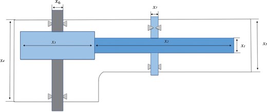
Speed reducer design.
Minimize:
subject to:
with bounds:
Table 16 reports the comparative results for the speed reducer design problem. Among all algorithms, ESCSA, together with ESC and COA, achieves the best fitness (2.995E + 03) across the mean, worst, and median metrics. ESCSA also obtains the smallest standard deviation (5.765E − 02), indicating the highest stability. In the Friedman mean rank test, COA ranks first, ESCSA ranks second, and ESC ranks third. The Wilcoxon rank-sum test (with ESCSA as the baseline) shows that ESCSA performs similarly to COA and ESC (both marked “(=)”, p ≥ 0.05), while significantly outperforming all other algorithms (marked “(+)”, p < 0.05). Overall, ESCSA is among the most effective and most stable solvers for this engineering problem. The optimal design variables obtained by each algorithm are reported in Table 17.
Comparative results for speed reducer design.
| Algorithm | Mean | Best | Worst | Median | Std | Friedman ranking | Wilcoxon |
|---|---|---|---|---|---|---|---|
| WOA | 3.402E + 03 | 3.011E + 03 | 5.381E + 03 | 3.158E + 03 | 6.355E + 02 | 7 | (+) |
| COA | 3.002E + 03 | 2.994E + 03 | 3.034E + 03 | 2.995E + 03 | 1.414E + 01 | 1 | (=) |
| HHO | 3.940E + 03 | 3.017E + 03 | 5.303E + 03 | 3.801E + 03 | 6.925E + 02 | 9 | (+) |
| MELGWO | 2.999E + 03 | 2.995E + 03 | 3.009E + 03 | 2.999E + 03 | 3.340E + 00 | 4 | (+) |
| HO | 3.042E + 03 | 2.995E + 03 | 3.190E + 03 | 3.032E + 03 | 6.500E + 01 | 6 | (+) |
| FGO | 3.972E + 03 | 3.353E + 03 | 4.674E + 03 | 4.060E + 03 | 3.765E + 02 | 11 | (+) |
| HLOA | 3.236E + 03 | 2.998E + 03 | 5.620E + 03 | 3.032E + 03 | 5.967E + 02 | 5 | (+) |
| GGO | 4.011E + 03 | 3.033E + 03 | 5.348E + 03 | 4.288E + 03 | 8.604E + 02 | 9 | (+) |
| CTCM | 3.171E + 03 | 3.058E + 03 | 3.226E + 03 | 3.190E + 03 | 4.087E + 01 | 10 | (+) |
| ESC | 2.995E + 03 | 2.995E + 03 | 2.995E + 03 | 2.995E + 03 | 6.058E − 02 | 3 | (=) |
| ESCSA | 2.995E + 03 | 2.995E + 03 | 2.995E + 03 | 2.995E + 03 | 5.765E − 02 | 2 | \ |
Note: Bold values indicate the best result.
Optimal solutions obtained by each algorithm for the speed reducer design problem.
| Algorithm | Best fitness | |${{x}_1}$| | |${{x}_2}$| | |${{x}_3}$| | |${{x}_4}$| | |${{x}_5}$| | |${{x}_6}$| | |${{x}_7}$| |
|---|---|---|---|---|---|---|---|---|
| WOA | 3011.759 | 3.512996 | 0.700000 | 17.000000 | 7.528178 | 7.724716 | 3.357388 | 5.286658 |
| COA | 2994.424 | 3.500000 | 0.700000 | 17.000000 | 7.300000 | 7.715320 | 3.350541 | 5.286654 |
| HHO | 3017.061 | 3.500000 | 0.700000 | 17.000000 | 7.534429 | 7.791673 | 3.357111 | 5.322907 |
| MELGWO | 2995.284 | 3.500621 | 0.700000 | 17.000000 | 7.300000 | 7.723121 | 3.350572 | 5.287342 |
| HO | 2995.343 | 3.500003 | 0.700000 | 17.000000 | 7.300000 | 7.767279 | 3.351071 | 5.287035 |
| FGO | 3353.192 | 3.579969 | 0.713383 | 18.053756 | 7.967143 | 7.868745 | 3.413828 | 5.363255 |
| HLOA | 2997.840 | 3.500031 | 0.700000 | 17.008844 | 7.303701 | 7.715320 | 3.357757 | 5.286653 |
| GGO | 3032.749 | 3.510655 | 0.700000 | 17.000000 | 7.300000 | 7.724300 | 3.492407 | 5.287061 |
| CTCM | 3058.314 | 3.505455 | 0.700000 | 17.000000 | 7.300000 | 7.740184 | 3.546095 | 5.287323 |
| ESC | 2994.480 | 3.500006 | 0.700000 | 17.000000 | 7.300355 | 7.716473 | 3.350558 | 5.286687 |
| ESCSA | 2994.445 | 3.500025 | 0.700000 | 17.000000 | 7.300193 | 7.715347 | 3.350547 | 5.286664 |
5.1.2. Multi-disc clutch braking problem
This is a common constrained engineering design problem in vehicle engineering. The main objective of this problem is to minimize the mass of a multiple-disc clutch brake. The five variables are: inner diameter |${{r}_i}$|, outer diameter |${{r}_o}$|, brake disc thickness t, driving force F, and surface friction coefficient Z. The specific structure is shown in Figure 13. The mathematical formulation of the multi-disc clutch braking problem is given in Equation 19.
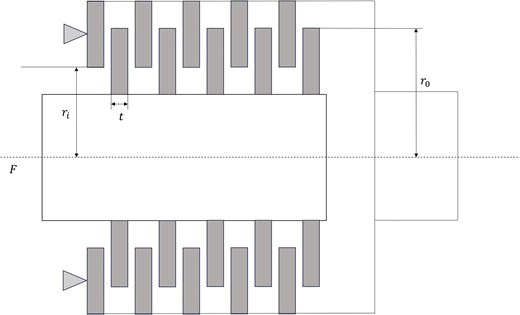
Diagram of the multi-disc clutch braking problem.
Consider:
Objective function:
Subject to:
Variable range:
Table 18 summarizes the results for the multiple-disc clutch brake problem. The optimal fitness value (0.235242) is attained by seven algorithms (WOA, HHO, MELGWO, HLOA, ESC, ESCSA, and also COA in its best and median runs). ESCSA, together with WOA, HHO, MELGWO, HLOA, and ESC, achieves the best possible mean, best, worst, and median values. In the Friedman ranking, ESC ranks first, COA second, ESCSA third, and HHO fourth. The Wilcoxon rank-sum test indicates that ESCSA performs comparably to ESC, COA, and HHO (all marked “(=)”, p ≥ 0.05), while being significantly better than MELGWO, HO, HLOA, GGO, and CTCM (marked “(+)”, p < 0.05). The FGO solution violates the constraints and is therefore excluded from the statistics (as noted in the table). The optimal design variables for each feasible algorithm are listed in Table 19.
Comparative results for the multi-disc clutch braking problem (bold values indicate the best result).
| Algorithm | Mean | Best | Worst | Median | Std | Friedman ranking | Wilcoxon |
|---|---|---|---|---|---|---|---|
| WOA | 2.352E − 01 | 2.352E − 01 | 2.352E − 01 | 2.352E − 01 | 1.359E − 06 | 7 | (+) |
| COA | 2.448E-01 | 2.352E − 01 | 3.308E − 01 | 2.352E − 01 | 2.916E − 02 | 2 | (=) |
| HHO | 2.352E − 01 | 2.352E − 01 | 2.352E − 01 | 2.352E − 01 | 3.898E − 07 | 4 | (=) |
| MELGWO | 2.352E − 01 | 2.352E − 01 | 2.352E − 01 | 2.352E − 01 | 1.366E − 07 | 5 | (+) |
| HO | 2.353E-01 | 2.352E − 01 | 2.354E − 01 | 2.353E − 01 | 2.700E − 05 | 10 | (+) |
| FGO | \ | \ | \ | \ | \ | \ | \ |
| HLOA | 2.352E − 01 | 2.352E − 01 | 2.352E − 01 | 2.352E − 01 | 2.667E − 10 | 6 | (+) |
| GGO | 2.368E−01 | 2.353E−01 | 2.402E − 01 | 2.362E − 01 | 1.330E − 03 | 9 | (+) |
| CTCM | 2.361E−01 | 2.353E − 01 | 2.384E − 01 | 2.359E − 01 | 7.714E − 04 | 8 | (+) |
| ESC | 2.352E − 01 | 2.352E − 01 | 2.352E − 01 | 2.352E − 01 | 5.584E − 09 | 1 | (=) |
| ESCSA | 2.352E − 01 | 2.352E − 01 | 2.352E − 01 | 2.352E − 01 | 8.615E − 08 | 3 | \ |
Note: The solution of FGO violates the constraints of the engineering problem, so its data are not included in the statistics.
Optimal solutions obtained by each algorithm for the multiple-disc clutch brake problem.
| Algorithm | Best fitness | |${{x}_1}$| | |${{x}_2}$| | |${{x}_3}$| | |${{x}_4}$| | |${{x}_5}$| |
|---|---|---|---|---|---|---|
| WOA | 0.235242 | 69.999999 | 90.000000 | 1.000000 | 930.244239 | 2.000000 |
| COA | 0.235242 | 70.000000 | 90.000000 | 1.000000 | 445.136302 | 2.000000 |
| HHO | 0.235242 | 70.000000 | 90.000000 | 1.000000 | 37.838528 | 2.000000 |
| MELGWO | 0.235242 | 70.000000 | 90.000000 | 1.000000 | 459.139312 | 2.000000 |
| HO | 0.235242 | 69.988708 | 90.000000 | 1.000000 | 506.532762 | 2.000000 |
| FGO | \ | \ | \ | \ | \ | \ |
| HLOA | 0.235242 | 70.000000 | 90.000000 | 1.000000 | 98.494498 | 2.000000 |
| GGO | 0.235291 | 69.995243 | 90.000000 | 1.000000 | 1000.000000 | 2.000000 |
| CTCM | 0.235311 | 69.993312 | 90.000000 | 1.000000 | 453.589639 | 2.000000 |
| ESC | 0.235242 | 70.000000 | 90.000000 | 1.000000 | 648.496465 | 2.000000 |
| ESCSA | 0.235242 | 70.000000 | 90.000000 | 1.000000 | 571.551569 | 2.000000 |
Note: The solution of FGO violates the constraints of the engineering problem, so its data are not included in the statistics.
5.1.3. Rolling element bearing design
The primary objective of this optimization problem is to maximize the load-carrying capacity of a rolling element bearing. The solution involves ten variables in total: five core design variables and five auxiliary design parameters. Specifically, the five design variables directly influencing the bearing’s structural performance are defined as Equation 20. pitch diameter of the bearing (denoted as |${{D}_m}$|), diameter of the rolling balls (|${{D}_b}$|), curvature coefficients of the outer and inner raceways (|${{f}_0}$| for the outer raceway and |${{f}_1}$| for the inner raceway), and the total number of rolling balls (Z). Complementing these, the five design parameters—including eccentricity coefficient (e), clearance coefficient (|$\varepsilon$|), width coefficient (|$\zeta$|), maximum diameter coefficient (|${{K}_{\text{Dmax}}}$|), and minimum diameter coefficient (|${{K}_{\text{Dmin}}}$|)—do not directly shape the bearing’s core structure but play a critical role in constraint formulation. The specific structure is shown in Figure 14.
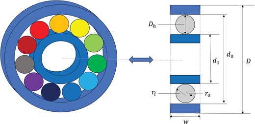
Rolling element bearing design.
Maximize:
subject to:
where
with bounds:
The results for the rolling element bearing design are shown in Table 20. ESCSA demonstrates outstanding performance, achieving the best results across all metrics. ESCSA maintains consistent performance across its “mean,” “best,” “worst,” and “median” metrics, with values of 1.696E + 04, and exhibits the lowest standard deviation of 7.655E-02, indicating minimal variability. These attributes propel ESCSA to the top of the Friedman ranking, outperforming all other algorithms. ESC ranks second in the Friedman test; its results closely match ESCSA’s across all metrics, but its standard deviation is slightly higher, indicating less stability. According to the Wilcoxon rank sum test results, only ESC shows marginally worse performance than ESCSA (marked “(=)”, p ≥ 0.05). At the same time, all other algorithms exhibit significantly inferior performance compared to ESCSA; the optimal design variables are reported in Table 21.
Comparative results for rolling element bearing design.
| Algorithm | Mean | Best | Worst | Median | Std | Friedman Ranking | Wilcoxon |
|---|---|---|---|---|---|---|---|
| WOA | 1.946E + 04 | 1.705E + 04 | 2.604E + 04 | 1.798E + 04 | 2.954E + 03 | 6 | (+) |
| COA | 1.746E + 04 | 1.696E + 04 | 1.798E + 04 | 1.706E + 04 | 4.356E + 02 | 3 | (+) |
| HHO | 1.855E + 04 | 1.699E + 04 | 3.024E + 04 | 1.706E + 04 | 3.408E + 03 | 8 | (+) |
| MELGWO | 1.700E + 04 | 1.696E + 04 | 1.706E + 04 | 1.699E + 04 | 2.745E + 01 | 4 | (+) |
| HO | 1.737E + 04 | 1.696E + 04 | 1.911E + 04 | 1.729E + 04 | 4.627E + 02 | 5 | (+) |
| FGO | 3.136E + 04 | 2.266E + 04 | 3.844E + 04 | 3.349E + 04 | 5.052E + 03 | 11 | (+) |
| HLOA | 2.188E + 04 | 1.698E + 04 | 4.032E + 04 | 2.226E + 04 | 5.232E + 03 | 9 | (+) |
| GGO | 2.280E + 04 | 1.841E + 04 | 2.906E + 04 | 2.281E + 04 | 2.284E + 03 | 10 | (+) |
| CTCM | 1.725E + 04 | 1.706E + 04 | 1.796E + 04 | 1.718E + 04 | 2.039E + 02 | 7 | (+) |
| ESC | 1.696E + 04 | 1.696E + 04 | 1.696E + 04 | 1.696E + 04 | 1.278E-01 | 2 | (=) |
| ESCSA | 1.696E + 04 | 1.696E + 04 | 1.696E + 04 | 1.696E + 04 | 7.655E-02 | 1 | \ |
Note: Bold values indicate the best result.
Optimal solutions obtained by each algorithm for the rolling element bearing design problem.
| Algorithm | Best fitness | |${{D}_m}$| | |${{D}_b}$| | Z | |${{f}_i}$| | |${{f}_o}$| | |${{K}_{\textit{Dmin}}}$| | |${{K}_{\textit{Dmax}}}$| | |$\varepsilon$| | e | |$\chi$| |
|---|---|---|---|---|---|---|---|---|---|---|---|
| WOA | 17047.03 | 129.677064 | 18.034880 | 4.510000 | 0.600000 | 0.600000 | 0.500000 | 0.600000 | 0.300000 | 0.089075 | 0.600000 |
| COA | 16958.20 | 131.200000 | 18.000000 | 4.525543 | 0.600000 | 0.600000 | 0.400000 | 0.699877 | 0.300000 | 0.048067 | 0.600000 |
| HHO | 16985.37 | 129.690506 | 18.000000 | 4.666553 | 0.600000 | 0.600000 | 0.400000 | 0.600000 | 0.300000 | 0.065035 | 0.600000 |
| MEL GWO | 16963.21 | 130.960578 | 18.000545 | 4.510038 | 0.600000 | 0.600000 | 0.446650 | 0.700000 | 0.300006 | 0.041013 | 0.600003 |
| HO | 16961.41 | 129.823804 | 18.000140 | 4.510127 | 0.600000 | 0.600000 | 0.458051 | 0.686715 | 0.312810 | 0.070068 | 0.600004 |
| FGO | 22660.94 | 129.972778 | 18.243735 | 4.679000 | 0.547913 | 0.548443 | 0.412892 | 0.643294 | 0.303886 | 0.029039 | 0.606096 |
| HLOA | 16978.24 | 129.999995 | 18.000000 | 4.867813 | 0.600000 | 0.600000 | 0.400000 | 0.600000 | 0.300000 | 0.020000 | 0.600000 |
| GGO | 18408.05 | 127.019299 | 18.325674 | 4.805764 | 0.591396 | 0.583972 | 0.404501 | 0.632666 | 0.301295 | 0.052938 | 0.601833 |
| CTCM | 17058.77 | 125.000000 | 18.000000 | 4.510000 | 0.600000 | 0.600000 | 0.448760 | 0.600000 | 0.300000 | 0.100000 | 0.600000 |
| ESC | 16958.34 | 131.198176 | 18.000057 | 4.705674 | 0.600000 | 0.600000 | 0.482910 | 0.623137 | 0.300001 | 0.044050 | 0.600000 |
| ESCSA | 16958.20 | 131.200000 | 18.000000 | 4.968062 | 0.600000 | 0.600000 | 0.471312 | 0.618464 | 0.300000 | 0.071796 | 0.600000 |
5.2. Experimental analysis of path planning in complex static environmental grid maps
In the robot path planning scenario, the mobile robot must navigate from its start to the goal while avoiding obstacles. Each feasible path is a sequence of evacuee steps, and the shortest collision-free path corresponds to the safest and fastest exit. The grid-based environment is treated as a discrete evacuation map, where blocked cells represent dangerous areas and free cells are passable corridors.
To validate the feasibility and effectiveness of ESCSA for path planning of mobile robots in complex grid maps, experiments were conducted across three grid scales: 40 × 40, 80 × 80, and 90 × 90. Simulation comparisons were performed using ESCSA alongside WOA, COA, HHO, MELGWO, HO, FGO, HLOA, GGO, CTCM, and the original ESC. To minimize the impact of algorithmic randomness on simulation results, each algorithm in this section was run independently 30 times under identical conditions. The table summarizes the average path length, minimum, maximum, median, and standard deviation across 30 independent runs for each algorithm. The best value for each metric is shown in bold. To more clearly compare their performance and determine whether ESCSA exhibits a significant advantage over other algorithms, this study also employs Friedman’s ranking. This ranking method sorts algorithms by performance in each run, calculates the average rank, and then ranks the 11 algorithms by their average ranks. Using ESCSA as the benchmark, a Wilcoxon rank-sum test is conducted at the 5% significance level.
Common map modeling approaches include grid-based mapping, topological mapping, and free-space methods (Liu et al., 2023; Qin et al., 2023). This paper comprehensively evaluated factors such as simplicity, intuitiveness, effectiveness, and ease of implementation, ultimately selecting the grid method to construct a model of the robot’s real-world environment, thereby generating a two-dimensional grid map. In this model, black grid cells represent obstacles, while white grid cells denote navigable areas. The robot is programmed to move in eight surrounding directions. If an obstacle is detected in any direction during movement, the corresponding path is deemed impassable.
Figure 15 illustrates the robot’s navigable states within a grid map. Red dots represent the robot at different positions, with arrows indicating the directions it can move. Specifically, the robot on the left can move freely in all 8 directions since no obstacles block its path. In contrast, the robot on the right can only move in the remaining 6 directions due to obstacles above and to its lower left. The three grid environments discussed in this paper feature obstacles arranged in a small and dense layout. This configuration generates an extremely large number of paths from the start to the end point, as each obstacle encountered branches into multiple routes to the destination, significantly increasing the likelihood that the algorithm will get stuck in local optima.
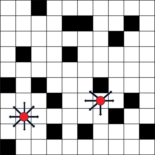
2D Raster Map.
In the grid-based path planning experiments, a path is represented as a sequence of intermediate waypoints. The robot always starts at the fixed start cell (1, 1) and ends at the fixed goal cell (N, N), where N is the grid size (40, 80, or 90). Each candidate solution (individual) is encoded as a vector of length |$N - 2$|, where the j-th element (|$j = 1,\ldots ,\ N - 2$|) specifies the row index of the waypoint in column |$j + 1$| (the first and last columns are fixed to the start and goal rows, respectively). All row indices are constrained to lie on free cells (i.e., cells with |$G( {row,\ col} ) = 0$|); the fitness function evaluates the quality of a candidate path as follows:
Collision penalty: If any intermediate waypoint falls on an obstacle, a large constant penalty |${{C}_{{\rm{collision}}}} = N \times N$| is added for each such collision. This ensures that infeasible paths are strongly discouraged.
Path generation for collision-free candidates: If all waypoints are collision-free, the algorithm constructs a continuous path by connecting consecutive waypoints with straight-line segments. When a segment would cross an obstacle, additional intermediate points are inserted to route around the obstacle while remaining in free cells.
Path smoothing: The continuous path is then passed through a smoothing procedure. This procedure iteratively checks each triple of consecutive path points (|${{p}_{i - 1}},\ {{p}_i},\ {{p}_{i + 1}}$|); if the straight line from |${{p}_{i - 1}}$| to |${{p}_{i + 1}}$| does not intersect any obstacle, the intermediate point |${{p}_i}$| is removed. This reduces the number of turns and produces a shorter, more robot-friendly trajectory.
- Fitness value: For a valid (collision-free) path, the fitness is defined as the total Euclidean length of the smoothed path, with Equation 21:(21)$$\begin{eqnarray} f\left( {{\rm{path}}} \right) = \mathop \sum \limits_{k = 1}^{L - 1} \sqrt {{{{\left( {{{x}_{k + 1}} - {{x}_k}{{)}^2} + ({{y}_{k + 1}} - {{y}_k}} \right)}}^2}}, \end{eqnarray}$$
where (|${{x}_k},\ {{y}_k}$|) are the coordinates of the k-th point in the smoothed path, and L is the number of points. This objective directly minimizes the travel distance. No additional corner cost is imposed because the smoothing process already favors straighter paths.
All compared algorithms (including ESCSA and the 10 baseline algorithms) use the same fitness function and path generation/smoothing routines, ensuring a fair comparison. Especially, for a grid of size |$N \times N$|, the number of intermediate waypoints (i.e., the dimension of the optimization problem) is |$N - 2$|. Thus, the problem dimensionality is 38, 78, and 88 for the 40 × 40, 80 × 80, and 90 × 90 grids, respectively.
5.2.1. 40 × 40 grid environment
In the 40 × 40 grid environment, the starting point is (1, 1) and the endpoint is (40, 40). Simulation experiments were conducted using the ESCSA algorithm alongside 10 comparison algorithms. The resulting paths for selected algorithms are visualized in Figure 16, and the quantitative results are summarized in Table 22.
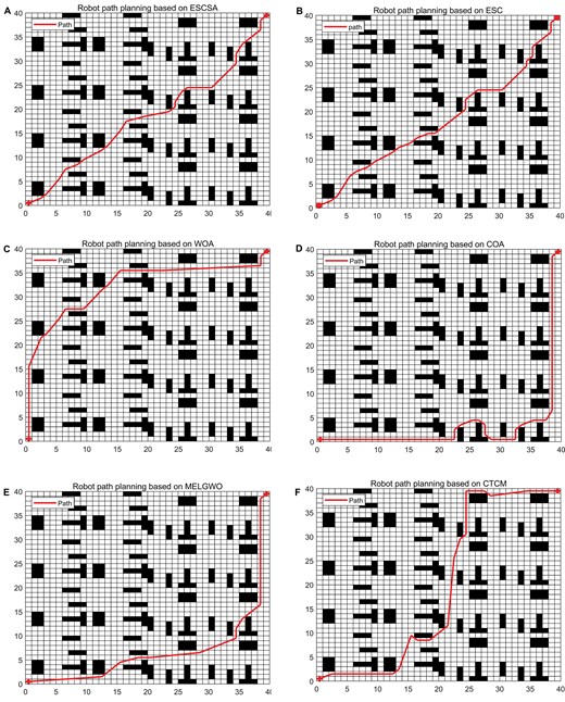
40 × 40 grid map planning paths. (A) ESCSA. (B) ESC. (C) WOA. (D) COA. (E) MELGWO. (F) CTCM.
The simulation results indicate that, compared to the ESC algorithm, the proposed ESCSA algorithm only slightly underperforms it in the “minimum value” metric among the five key indicators. Among all algorithms included in the comparison, ESCSA achieves the best overall performance across the mean, maximum, and median metrics, only slightly underperforming ESC in the minimum metric (by 0.23) and CTCM in the standard deviation (by 0.539). In the Friedman ranking, ESCSA ranked first, ESC second, MELGWO third, GGO fourth, WOA fifth, and HLOA sixth. The specific rankings are shown in Table 22. The Wilcoxon rank-sum test was used to assess significant differences between each algorithm and ESCSA. Except for ESC, all algorithms in the table showed significant differences (p < 0.05) and inferior performance compared to ESCSA. Although ESCSA outperformed ESC, the difference was not statistically significant. Furthermore, Figure 16 demonstrates that the paths planned by the ESCSA algorithm, in terms of both smoothness and the number of path turning points, outperformed the other ten comparison algorithms, yielding competitive results.
40 × 40 grid map simulation results.
| Algorithm | Mean | Min | Max | Median | Std | Friedman Ranking | Wilcoxon |
|---|---|---|---|---|---|---|---|
| WOA | 6.864E + 01 | 6.106E + 01 | 7.668E + 01 | 6.912E + 01 | 4.020E + 00 | 5 | (+) |
| COA | 7.901E + 01 | 6.241E + 01 | 8.324E + 01 | 8.078E + 01 | 5.014E + 00 | 10 | (+) |
| HHO | 7.470E + 01 | 7.025E + 01 | 7.943E + 01 | 7.413E + 01 | 2.221E + 00 | 9 | (+) |
| MELGWO | 6.470E + 01 | 5.826E + 01 | 7.154E + 01 | 6.500E + 01 | 3.006E + 00 | 3 | (+) |
| HO | 6.995E + 01 | 6.662E + 01 | 7.323E + 01 | 7.004E + 01 | 1.692E + 00 | 7 | (+) |
| FGO | 9.868E + 01 | 7.998E + 01 | 1.146E + 02 | 9.974E + 01 | 8.392E + 00 | 11 | (+) |
| HLOA | 6.896E + 01 | 6.378E + 01 | 7.245E + 01 | 7.031E + 01 | 2.631E + 00 | 6 | (+) |
| GGO | 6.821E + 01 | 6.446E + 01 | 8.148E + 01 | 6.759E + 01 | 3.181E + 00 | 4 | (+) |
| CTCM | 7.094E + 01 | 6.745E + 01 | 7.376E + 01 | 7.098E + 01 | 1.287E + 00 | 8 | (+) |
| ESC | 6.058E + 01 | 5.630E + 01 | 6.654E + 01 | 6.055E + 01 | 2.646E + 00 | 2 | (=) |
| ESCSA | 5.942E + 01 | 5.643E + 01 | 6.335E + 01 | 5.964E + 01 | 1.826E + 00 | 1 | \ |
Note: Bold values indicate the best result.
5.2.2. 80 × 80 and 90 × 90 grid environments
In an 80 × 80 grid environment, the starting point was set to (1, 1), with endpoints at (80, 80) and (90, 90). Simulation experiments were conducted using the ESCSA algorithm alongside 10 comparison algorithms. Simulation results are shown in Figures 17 and 18. Data comparisons for the 11 algorithms are presented in Tables 23 and 24.
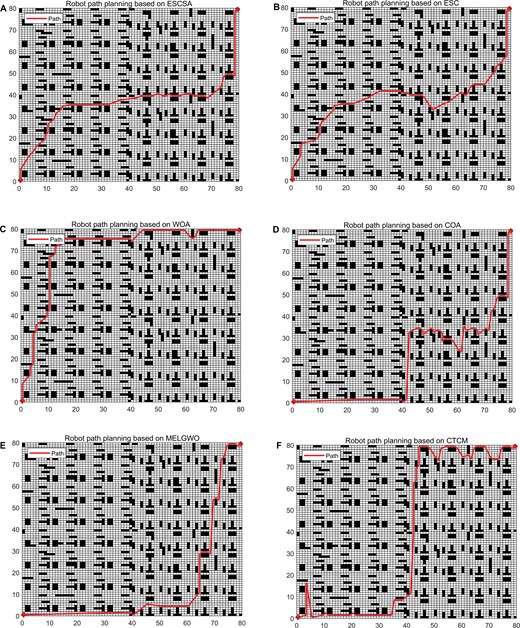
80 × 80 grid map planning paths. (A) ESCSA. (B) ESC. (C) WOA. (D) COA. (E) MELGWO. (F) CTCM.
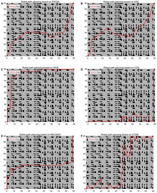
90 × 90 grid map planning paths. (A) ESCSA. (B) ESC. (C) WOA. (D) COA. (E) MELGWO. (F) CTCM.
The simulation results demonstrate that in an 80 × 80 grid environment, the proposed ESCSA algorithm exhibits significant advantages across multiple key performance metrics. Compared to ESC, ESCSA outperforms it across all five key metrics. The mean value most effectively reflects the overall performance advantage: ESCSA achieves 1.431E + 02, while ESC reaches 1.501E + 02, representing an approximately 5% improvement over ESC. Among all compared algorithms, only the standard deviation metric did not yield the best result for ESCSA (7.782E + 00). However, its value was within 3 points of HLOA (5.416E + 00), which achieved the best standard deviation. This fully demonstrates the excellence and exceptional stability of the ESCSA algorithm. In the Friedman ranking, ESCSA ranked first, ESC second, MELGWO third, WOA fourth, HLOA fifth, and HO sixth, as detailed in Table 23. The Wilcoxon rank-sum test confirms that ESCSA’s performance is statistically superior (|$p\ \,\lt\, \ 0.05$|) to that of all other algorithms, including ESC, in these more complex environments. This outcome reinforces ESCSA’s superiority, confirming its numerical advantage over other comparison algorithms while also establishing its statistically significant dominance.
80 × 80 grid map simulation results.
| Algorithm | Mean | Min | Max | Median | Std | Friedman Ranking | Wilcoxon |
|---|---|---|---|---|---|---|---|
| WOA | 1.546E + 02 | 1.369E + 02 | 1.873E + 02 | 1.538E + 02 | 1.037E + 01 | 4 | (+) |
| COA | 1.794E + 02 | 1.662E + 02 | 1.958E + 02 | 1.759E + 02 | 8.992E + 00 | 9 | (+) |
| HHO | 1.690E + 02 | 1.586E + 02 | 1.880E + 02 | 1.676E + 02 | 6.193E + 00 | 8 | (+) |
| MELGWO | 1.531E + 02 | 1.386E + 02 | 1.662E + 02 | 1.522E + 02 | 7.592E + 00 | 3 | (+) |
| HO | 1.581E + 02 | 1.506E + 02 | 1.680E + 02 | 1.561E + 02 | 5.143E + 00 | 6 | (+) |
| FGO | 3.180E + 02 | 2.674E + 02 | 3.647E + 02 | 3.171E + 02 | 2.434E + 01 | 11 | (+) |
| HLOA | 1.565E + 02 | 1.480E + 02 | 1.680E + 02 | 1.547E + 02 | 5.416E + 00 | 5 | (+) |
| GGO | 1.659E + 02 | 1.531E + 02 | 2.183E + 02 | 1.640E + 02 | 1.158E + 01 | 7 | (+) |
| CTCM | 2.072E + 02 | 1.721E + 02 | 2.433E + 02 | 2.092E + 02 | 1.805E + 01 | 10 | (+) |
| ESC | 1.511E + 02 | 1.378E + 02 | 1.728E + 02 | 1.495E + 02 | 1.105E + 01 | 2 | (+) |
| ESCSA | 1.436E + 02 | 1.287E + 02 | 1.610E + 02 | 1.417E + 02 | 7.782E + 00 | 1 | \ |
Note: Bold values indicate the best result.
The 90 × 90 grid environment slightly increases map complexity compared to the 80 × 80 grid environment. Statistical comparisons of algorithmic performance show that results in the 90 × 90 grid environment are similar to those in the 80 × 80 environment, and that Friedman rankings remain consistent across environments. Compared to the 80 × 80 grid environment, MELGWO dropped from third to fifth, while HLOA moved up from fifth to third. The remaining rankings remain unchanged. The Wilcoxon rank-sum test results align with those from the 80 × 80 grid environment, further validating ESCSA’s consistent advantage in path planning in complex environments.
90 × 90 grid map simulation results.
| Algorithm | Mean | Min | Max | Median | Std | Friedman ranking | Wilcoxon |
|---|---|---|---|---|---|---|---|
| WOA | 1.772E + 02 | 1.559E + 02 | 2.234E + 02 | 1.716E + 02 | 1.661E + 01 | 4 | (+) |
| COA | 2.274E + 02 | 2.020E + 02 | 2.561E + 02 | 2.266E + 02 | 1.395E + 01 | 9 | (+) |
| HHO | 2.257E + 02 | 1.904E + 02 | 2.539E + 02 | 2.282E + 02 | 1.126E + 01 | 8 | (+) |
| MELGWO | 1.803E + 02 | 1.622E + 02 | 2.192E + 02 | 1.732E + 02 | 1.725E + 01 | 5 | (+) |
| HO | 1.796E + 02 | 1.700E + 02 | 1.941E + 02 | 1.788E + 02 | 7.478E + 00 | 6 | (+) |
| FGO | 3.834E + 02 | 2.956E + 02 | 4.446E + 02 | 3.861E + 02 | 3.257E + 01 | 11 | (+) |
| HLOA | 1.762E + 02 | 1.670E + 02 | 2.015E + 02 | 1.758E + 02 | 6.556E + 00 | 3 | (+) |
| GGO | 2.089E + 02 | 1.909E + 02 | 2.707E + 02 | 2.027E + 02 | 1.902E + 01 | 7 | (+) |
| CTCM | 2.699E + 02 | 2.240E + 02 | 3.195E + 02 | 2.648E + 02 | 2.366E + 01 | 10 | (+) |
| ESC | 1.710E + 02 | 1.489E + 02 | 1.997E + 02 | 1.701E + 02 | 1.041E + 01 | 2 | (+) |
| ESCSA | 1.614E + 02 | 1.470E + 02 | 1.857E + 02 | 1.599E + 02 | 1.002E + 01 | 1 | \ |
Note: Bold values indicate the best result.
Combining experimental results across three grid environments, the ESCSA algorithm demonstrates comprehensive, stable, and superior performance. In the 40 × 40 environment, ESCSA achieved the highest overall ranking, though its advantage over ESC was not statistically significant. As environmental complexity increased in the 80 × 80 and 90 × 90 grids, ESCSA’s superiority became decisive, significantly outperforming all competitors, including ESC. This demonstrates ESCSA’s enhanced capability for solving complex path-planning problems.
5.2.3. Effect size analysis for practical significance
To complement the statistical significance tests (Wilcoxon rank sum) reported in Tables 22–24, the practical relevance of the performance differences is further quantified using standardized effect size measures. Following recent recommendations in the metaheuristic literature (Arcuri & Briand, 2014; Ismail & Omran, 2026), Cliff’s δ (non-parametric, robust to outliers) and Cohen’s d (parametric, standardized mean difference) are adopted. For completeness, the relative improvement percentage (RIP) is also reported, which provides an intuitive engineering interpretation.
Let |${\rm{X}} = \{ {{{x}_1},{{x}_2},\ldots ,{{x}_n}} \}$| denotes the set of path lengths obtained by ESCSA over |$n = 30$| independent runs, and |${\rm{Y}} = \{ {{{y}_1},{{y}_2},\ldots ,{{y}_n}} \}$| denotes the corresponding set from a competing algorithm.
- Cliff’s δ with Equation 22:(22)$$\begin{eqnarray} \delta = \frac{{\# ({{x}_i} \,\gt\, {{y}_j}) - \# ({{x}_i} \,\lt\, {{y}_j})}}{{{{n}^2}}}, \end{eqnarray}$$
where |$\# ({{x}_i} \,\gt\, {{y}_j})$| counts the number of pairs |$( {i{\rm{,}}j} )$| with |${{x}_i} \,\gt\, {{y}_j}$|, and |$\# ({{x}_i} \,\lt\, {{y}_j})$| counts the number of pairs with |${{x}_i} \,\lt\, {{y}_j}$| (ties are ignored); the comparisons are made over all |$n \times n$| pairs. A positive δ indicates that ESCSA tends to outperform the competitor. Magnitude interpretation: |$\mid \delta \mid \,\lt\, 0.147$| negligible, |$0.147 \le \mid \delta \mid \,\lt\, 0.33$| small, |$0.33 \le \mid \delta \mid \,\lt\, 0.474$| medium, |$\mid \delta \mid \ge 0.474$| large.
- Cohen’s d with Equation 23:(23)$$\begin{eqnarray} d = \frac{\bar{Y} - \bar{X}}{{\sqrt {\frac{{s_X^2 + s_Y^2}}{2}} }}, \end{eqnarray}$$
where |$\bar{ X}$|and |$\bar{Y}$| are their respective sample means. |$s_X^2$| and |$s_Y^2$| are their sample variances. A positive d indicates that ESCSA achieves a lower (better) mean path length. For Cohen’s d, |$\mid d\mid \ge 0.2$|, |$0.5$|, and |$0.8$| indicate small, medium, and large effects, respectively.
- Relative improvement percentage (RIP) with Equation 24:(24)$$\begin{eqnarray} {\rm{RIP}}\left( {\rm{\% }} \right) = \frac{\bar{X}-\bar{Y}}{\bar{X}} \times 100{\rm{\%}}. \end{eqnarray}$$
A negative value indicates ESCSA outperforms the competitor.
Effect size analysis (Cliff’s δ, Cohen’s d, RIP) and Wilcoxon significance for path planning experiments.
| Algorithm | Map | Cliff’s δ | Effect strength | Cohen’s d | RIP (%) | Wilcoxon (vs ESCSA) |
|---|---|---|---|---|---|---|
| ESC | 40 × 40 | 0.33 | Medium | 0.39 | –0.51 | (=) p = 0.480 |
| 80 × 80 | 0.59 | Large | 0.77 | –5.17 | (+) p = 0.002 | |
| 90 × 90 | 0.64 | Large | 0.83 | –5.46 | (+) p = 0.003 | |
| MELGWO | 40 × 40 | 0.67 | Large | 1.13 | –8.90 | (+) |
| 80 × 80 | 0.69 | Large | 1.14 | –6.63 | (+) | |
| 90 × 90 | 0.72 | Large | 1.10 | –10.81 | (+) | |
| WOA | 40 × 40 | 0.76 | Large | 2.24 | –14.77 | (+) |
| 80 × 80 | 0.72 | Large | 1.03 | –7.75 | (+) | |
| 90 × 90 | 0.73 | Large | 1.06 | –10.86 | (+) | |
| HLOA | 40 × 40 | 0.75 | Large | 2.53 | –16.32 | (+) |
| 80 × 80 | 0.76 | Large | 1.62 | –9.28 | (+) | |
| 90 × 90 | 0.72 | Large | 1.40 | –9.37 | (+) | |
| HO | 40 × 40 | 0.81 | Large | 2.75 | –17.89 | (+) |
| 80 × 80 | 0.78 | Large | 1.77 | –10.01 | (+) | |
| 90 × 90 | 0.77 | Large | 1.66 | –11.52 | (+) | |
| CTCM | 40 × 40 | 0.83 | Large | 2.96 | –19.32 | (+) |
| 80 × 80 | 0.95 | Large | 3.70 | –44.21 | (+) | |
| 90 × 90 | 0.97 | Large | 4.71 | –64.60 | (+) | |
| HHO | 40 × 40 | 0.88 | Large | 3.17 | –24.87 | (+) |
| 80 × 80 | 0.88 | Large | 2.67 | –18.79 | (+) | |
| 90 × 90 | 0.93 | Large | 4.56 | –38.99 | (+) | |
| GGO | 40 × 40 | 0.77 | Large | 2.00 | –13.53 | (+) |
| 80 × 80 | 0.83 | Large | 1.59 | –15.45 | (+) | |
| 90 × 90 | 0.90 | Large | 2.67 | –30.39 | (+) | |
| COA | 40 × 40 | 0.93 | Large | 4.19 | –33.53 | (+) |
| 80 × 80 | 0.91 | Large | 2.98 | –25.80 | (+) | |
| 90 × 90 | 0.93 | Large | 4.05 | –40.46 | (+) | |
| FGO | 40 × 40 | 0.96 | Large | 5.60 | –67.90 | (+) |
| 80 × 80 | 0.99 | Large | 7.15 | –122.17 | (+) | |
| 90 × 90 | 0.99 | Large | 6.52 | –135.37 | (+) |
Note: Wilcoxon significance marks: (+) ESCSA significantly better (p < 0.05); (=) no significant difference (p ≥ 0.05). In the last column of the table, the p-values for the other algorithms are all less than 0.001, so they are not specifically labeled.
Table 25 summarizes the effect size metrics for all competing algorithms across the three grid environments (40 × 40, 80 × 80, 90 × 90). The corresponding Wilcoxon significance marks (from Tables 22–24) are also included for reference. In the 40 × 40 grid, ESCSA exhibits a medium positive effect against ESC (Cliff’s δ = 0.33, Cohen’s d = 0.39), and a large positive effect against all other algorithms (δ ≥ 0.67). The relative improvement over ESC is only 0.51% and not statistically significant (p = 0.48), confirming that ESC and ESCSA perform nearly equivalently in this small map. As the grid size increases to 80 × 80 and 90 × 90, the advantage of ESCSA becomes consistently large (δ ≥ 0.59, d ≥ 0.77) against every competitor, including ESC. The relative improvements over ESC reach 5.17% (80 × 80) and 5.46% (90 × 90), and the Wilcoxon tests become significant (p < 0.01). This demonstrates that the enhancements introduced in ESCSA are particularly beneficial in larger, more complex environments.
Across all three maps, ESCSA shows overwhelmingly large effects (δ > 0.9, d > 3.0) against CTCM, COA, HHO, GGO, and FGO. These effect sizes confirm that the observed gains are practically substantial and not merely artifacts of statistical testing.
6. Conclusions and future works
Building upon the Escape (ESC) algorithm, this paper proposes a multi-strategy enhanced variant, termed ESCSA, which incorporates three key improvements: dynamic mask probability adjustment staged as 0.6 → 0.5 → 0.4, stagnation detection with SA local search triggered after |$T/25$| consecutive generations without significant relative improvement, and a worst-elimination strategy that injects |$N/6$| new individuals every |$T/10$| generations. The effectiveness of each strategy is validated through ablation experiments, diversity analysis, and exploration–exploitation balance analysis.
To evaluate the algorithm’s performance, ESCSA is compared against 10 state-of-the-art algorithms. On the CEC 2017 benchmark suite, ESCSA achieves the highest Friedman rankings across all dimensions. In three engineering design problems—speed reducer design, multi-disc clutch brake design, and rolling element bearing design—ESCSA ranks second, third, and first. In robot path planning across 40 × 40, 80 × 80, and 90 × 90 static grid environments, ESCSA consistently generates superior paths.
Despite its strong overall performance, ESCSA has several limitations that suggest promising directions for future research. First, the SA component relies on fixed parameters rather than problem-adaptive control; future work will introduce adaptive mechanisms to accommodate diverse problem characteristics better. Second, the current path planning study is limited to static environments; the comparisons are restricted to metaheuristic algorithms; and path quality could be further improved. Future work will deepen the application of ESCSA to robot path planning. Specific directions include algorithmic refinements tailored to this domain, path quality optimization, extension to dynamic environments, and hardware deployment on embedded navigation systems with real-world experimental validation. Third, the simple penalty function used for constraint handling, while effective for the problems tested, may produce infeasible intermediate solutions; more sophisticated constraint-handling techniques will be explored. Fourth, statistical rigor could be further enhanced through power analysis, confidence intervals, and multiple-comparison corrections, which are planned for future studies.
Conflicts of interest
The authors declare that they have no known competing financial interests or personal relationships that could have appeared to influence the work reported in this paper.
Author contributions
Ming Wang: Conceptualization, Writing—original draft, Software, Formal analysis, Visualization. Qipeng Chen: Conceptualization, Methodology, Writing—Review & Editing, Revise, Funding acquisition, Supervision. Silei Fan: Software, Validation. Ning Yu: Software, Visualization. Junqiang Zheng: Writing—Review & Editing, Supervision.
Funding
This work was supported by the Guizhou Provincial Basic Research Program (Natural Science) (Grant No. Qiankehejichu-ZK [2023] General 014; Grant No. MS〔2025〕087), the Growth Project for Young Scientific and Technological Talents in General Colleges and Universities of Guizhou Province (Grant No. Qianjiaoji [2022]306), and the Introducing Talents to Initiate Funded Research Projects of Guiyang University(Grant No. GYU-KY-[2026]).
Data availability
All data generated or analysed during this study are included in this manuscript. Additional datasets supporting the conclusions of this study are available from the corresponding author upon reasonable request.
Acknowledgments
The authors thank those people or institutions that have helped us in the preparation of the manuscript.


