


Abstract
This study introduces a novel non-systematic logical structure, termed B-type Random 2-Satisfiability, which incorporates non-redundant first- and second-order clauses, as well as redundant second-order clauses. The proposed logical rule is implemented in the discrete Hopfield neural network using the Wan Abdullah method, with the corresponding cost function minimized through an exhaustive search algorithm to reduce the inconsistency of the logical rules. The inclusion of redundant literals is intended to enhance the capacity of the model to extract overlapping knowledge. Additionally, the performance of B-type Random 2-Satisfiability with varying clause proportions in the discrete Hopfield neural network is evaluated using various metrics, including learning error, retrieval error, weight error, energy analysis, and similarity analysis. Experimental results indicate that the model demonstrates superior efficiency in synaptic weight management and offers a broader solution space when the number of the three types of clauses is selected randomly.
A B-type Random 2-Satisfiability (BRAN2SAT) logic is proposed, which is composed of both redundant and non-redundant literals.
The BRAN2SAT logic is embedded into a discrete Hopfield neural network using the WA method to enhance the interpretability of the network.
The performance of the proposed model is evaluated using various metrics.
A superior performance of BRAN2SAT was confirmed by the results.
1 Introduction
Artificial neural networks (ANNs) are mathematical models inspired by the perceptual processing of the human brain. Composed of interconnected neurons, ANNs adjust synaptic weights in response to external inputs, enabling the generation of accurate outputs for specific tasks (Rosenblatt 1958). Nowadays, ANNs have numerous applications, such as in natural language processing (Raza et al. 2024), autonomous driving (Xu et al. 2024), medical image processing (Lee et al. 2023; Azad et al. 2024), financial forecasting (Mousapour Mamoudan et al. 2023; Lee & Kang 2023), and smart manufacturing (Sakkaravarthi et al. 2024; Farahani et al. 2025). One of the earliest ANNs was the Hopfield neural network (HNN) proposed by Hopfield and Tank (Hopfield 1982). This single-layer feedback network lacks hidden layers and features neurons that form loops, allowing outputs to feed back into the input layer. The Discrete hopfield neural network (DHNN), a specific form of HNN, utilizes discrete binary states for neurons and features bidirectional connections through synaptic weights. It is trained with the Hebbian learning rule (Hopfield & Tank 1985), where neurons are iteratively updated until convergence to a near-optimal state. The asynchronous updating process ensures DHNN minimizes an energy function, leading to a stable state suitable for real-world problems (Ma et al. 2023; Yu et al. 2024; Wang et al. 2024a; Deng et al. 2024). However, as the number of neurons increases, the DHNN faces challenges such as local minima and limited storage capacity. Therefore, the structure of DHNN must be optimized and improved. To address the storage capacity limitations of conventional DHNN (approximately
Recent studies have proposed various non-systemic logics to address these limitations. These logics are composed of clauses that are randomly arranged in different orders, offering greater flexibility than system logic. This flexibility enables non-systemic logic to generate a wider diversity of neuron states, enhancing its adaptability to a wide range of real-world problems. Sathasivam et al. (2020) proposed Random k-Satisfiability (RAN2SAT), combining first- and second-order clauses. Although the quality of neuron states declines as the number of neurons increases, RAN2SAT exhibits greater variations in synaptic weights. Building on this idea, Zamri et al. (2022) proposed a new non-systematic logical rule, weighted Random 2-Satisfiability (
Maximum satisfiability (MAXSAT) is a variant of logical rules that is inherently unsatisfiable. According to Prugel-Bennett & Tayarani-Najaran (2011), MAXSAT aims to maximize the number of satisfiable clauses, the outcome of MAXSAT logic is consistently False. Kasihmuddin et al. (2018) first introduced non-satisfiability logic into DHNN through maximum 2-satisfiability (MAX2SAT), where only satisfiable clauses are considered in the cost function, as synaptic weights for non-satisfiable clauses are set to zero. This MAX2SAT approach, utilizing exhaustive search (ES), reportedly achieves global minimum energy for smaller neuron sets. Building on this, Someetheram et al. (2022) proposed a new non-satisfiability logic, Random maximum 2-satisfiability (RM2SAT), which combines MAX2SAT and Random 2-Satisfiability. RM2SAT is embedded in DHNN, employing the Election Algorithm during the learning phase to find a consistent interpretation that minimizes the cost function and achieves optimal performance in both learning and testing. While MAXSAT has been successfully applied in DHNN, no existing literature has explored the implementation of satisfiability logic with redundant literals in DHNN. Therefore, it is necessary to consider introducing redundant literals in satisfiability logic. On the one hand, logical rules with redundant literals can represent
As a follow-up to the previously mentioned literature review, it is worthwhile to investigate the following research questions:
What alternative representations of non-systematic logic can effectively simplify the structure of the DHNN by introducing redundant and non-redundant literals?
What alternative representations of non-systematic logic can precisely adjust synaptic weights through redundant literals, thereby effectively modelling neuron connections in the DHNN?
What experimental design and performance metrics are most suitable for validating the effectiveness of embedding non-systematic logical rules with redundant literals into the DHNN during the learning and retrieval phases?
To answer these questions, B-type Random 2-Satisfiability (BRAN2SAT) is proposed by incorporating redundant second-order clauses, as well as non-redundant second- and first-order clauses. The inclusion of redundant second-order clauses enables more diverse connections with fewer neurons in the DHNN and facilitates control over neuron state updates. This work represents the first application of logical rules with redundant literals in DHNN, demonstrating their potential to enhance network performance. The contributions of this study are as follows:
To propose a novel non-systematic logical rule termed BRAN2SAT. This logic consists of redundant second-order clauses combined with non-redundant first- and second-order clauses. This combination preserves the fault tolerance of redundant clauses and reflects the simplicity and efficiency of non-redundant clauses, which achieves equilibrium between logical complexity and reasoning efficiency.
To embed the proposed BRAN2SAT into the DHNN, each literal is mapped to the corresponding neuron in the network, forming the DHNN–BR2SAT model. The inconsistencies in BRAN2SAT are then minimized, and the correct synaptic weights of the DHNN are determined by comparing the associated cost function with the energy function. The influence of BRAN2SAT is reflected in the behaviour of the DHNN–BR2SAT through the synaptic weights.
To conduct extensive experiments to demonstrate the effectiveness of DHNN–BR2SAT. DHNN–BR2SAT is evaluated by considering different clause orders. The performance of the learning and retrieval phases of DHNN–BR2SAT is comprehensively evaluated in terms of the performance metrics of learning error, synaptic weight error, energy distribution, retrieval error, total variation, and similarity metrics to justify the behaviour of the proposed BRAN2SAT.
The rest of the study is structured as follows. Section 2 provides the motivation. Section 3 presents the overview structure of the novel BRAN2SAT. Section 4 explains the implementation of BRAN2SAT in DHNN. Section 5 displays the experimental setup and performance evaluation metrics employed in the whole simulation experiment. Section 6 explains the results, discusses the behaviour of DHNN combined with BRAN2SAT, and addresses the limitations of the model. Finally, Section 7 presents conclusions and future work.
2 Motivation
2.1 The satisfiability logic in the DHNN lacks redundant literals
A significant limitation of DHNN lies in their tendency to become trapped in local minima during energy descent, which hinders the ability of the network to recall stored patterns accurately. Embedding logical rules within DHNN enhances interpretability by guiding neuron update paths. Moreover, the final neuron states of the improved DHNN model offer potential solutions for practical optimization problems. Various types of logical rules have been successfully incorporated into DHNN, including systematic logical rules (Kasihmuddin et al. 2019; Mansor et al. 2017), non-systematic logical rules (Sathasivam et al. 2020), and hybrid logical rules (Guo et al. 2022; Gao et al. 2022). However, these rules are based on non-redundant literals, where each literal appears only once in the logical rules. Since each literal represents a neuron that connects to others as well as to itself, when literals appear only once, the associated neurons exhibit similar synaptic weights, lacking sufficient variability. This can lead to overfitting during the DHNN retrieval phase. To address this issue, the embedding of MAXSAT with two redundant variables of opposing values in DHNN achieves optimal performance in learning and retrieval phases (Kasihmuddin et al. 2018; Someetheram et al. 2022). However, the logic constrains the values and number of redundant variables, limiting their flexibility in regulating synaptic weights. To address these limitations, we propose a satisfiability logic that incorporates redundant literals. This is achieved by randomly generating redundant second-order clauses alongside non-redundant first- and second-order clauses, providing DHNN with more flexible logical rules. This approach provides a novel method for modelling in real-world applications.
2.2 Limited storage capacity of DHNN
The storage capacity of DHNN is relatively limited. Theoretically, the maximum capacity is approximately 15% of the total number of neurons
3 B-type Random 2-Satisfiability
BRAN2SAT is a non-systematic satisfiability logical rule with redundant literals, represented in conjunctive normal form (CNF). The logical structure comprises clauses containing two redundant literals and clauses with at most two non-redundant random literals. Literals are combined using the OR operator (
A set of
- A set of
- The formulation for Redundancy 2-satisfiability is presented as follows (Liberatore 2008):where(3)
- The formulation for Random 2-Satisfiability is given as:the clause of(6)
- The general formulation of
The four different examples for
According to Equations 10–13, the bipolar value for each literal of the CNF takes either 1 or −1, representing TRUE and FALSE, respectively (Sathasivam 2010). The logical formula is satisfied (i.e.
4 BRAN2SAT in the discrete Hopfield neural network
4.1 Learning phase
The DHNN is a fully interconnected feedback network consisting of a single layer of binary neurons. The neuron state is typically represented by a bipolar value of +1 or −1. The neuron update formula is as follows (Hopfield 1982):
from Equation 14,
where
where
where
4.2 Retrieval phase
During the retrieval phase, the neuron states are updated asynchronously. This iterative updating process is governed by Equations 18–20, as provided below:
where the local field
When the DHNN reaches a stable state, the energy function converges to the nearest local minimum. The Lyapunov energy function
where
To determine whether the final neuron state corresponds to the global minimum, the following formula is applied:
where
The stable state of a neural network refers to the condition in which, after a certain point in time, the neuron states no longer change, i.e.
Let
A stable state exists in the DHNN only if Theorem 4.1 is satisfied. Under this condition, the DHNN evolves in the direction of decreasing energy until a stable state is reached. The following provides proof that the energy function decreases monotonically.
The Lyapunov energy function for neuron
The change in energy from time
The energy change from
From Equation 18, we obtain
It follows that the DHNN evolves in the direction of Lyapunov energy function minimization.
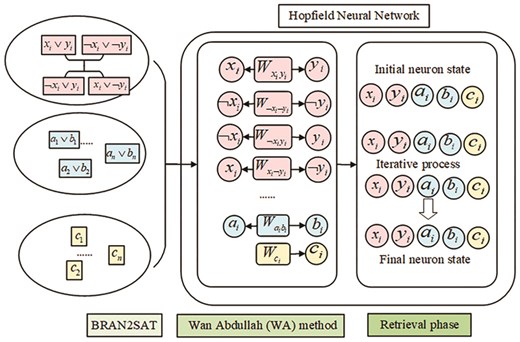
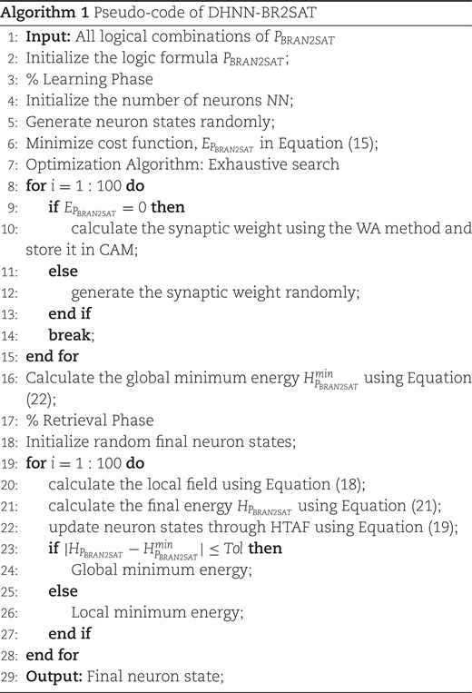
Figure 1 presents the schematic diagram of DHNN–BR2SAT. The model incorporates non-redundant first-, second-, and redundant second-order clauses. Algorithm 1 outlines the pseudo-code of DHNN–BR2SAT with an ES algorithm in the learning phase.
Schematic diagram of DHNN–BR2SAT.
5 Experimental setup
This section evaluates the impact of varying numbers of clauses at different orders on the behaviour of DHNN–BR2SAT through simulation experiments. The evaluation is conducted in three aspects: the learning phase, the retrieval phase, and both total variation and the similarity index. A comprehensive analysis is provided on how different logical orders affect BRAN2SAT performance, along with an evaluation of parameter perturbation.
The experiment was conducted in a Windows 11 Home Edition environment with an i5-1035G4 1.5GHz CPU and 8 GB RAM. MATLAB R2016b was used as the development tool. The detailed parameter settings for the algorithm are provided in Table 1.
Parameters for the proposed DHNN–BR2SAT.
| Parameter explanation | Parameter value |
|---|---|
| Number of neurons ( | |
| Number of neuron combinations ( | 100 (Zamri et al. 2020) |
| Number of learning trials ( | 100 |
| Current number of learning trials ( | |
| Initialization of neuron states in the learning phase | Random |
| Threshold ( | 0 (Zamri et al. 2022) |
| Relaxation rate ( | |
| Number of testing trials ( | 100 (Zamri et al. 2020) |
| Initialization of neuron states in the testing phase | Random |
| Tolerance value ( | 0.001 (Sathasivam 2010) |
| Activation function | HTAF |
| Type of selection | Random search |
To evaluate the efficiency of DHNN–BR2SAT, this section examines the performance of the model across five aspects: learning error analysis and weight analysis during the learning phase, energy analysis, and global solution analysis during the retrieval phase, and similarity index analysis. Tables 2–4 present the parameters associated with all evaluation metrics.
List of parameters in the learning phase.
| Parameter | Remarks |
|---|---|
| Maximum fitness achieved | |
| Current fitness achieved | |
| Synaptic weight obtained by WA method | |
| Current synaptic weight | |
| Number of weights at a time | |
| Parameter | Remarks |
|---|---|
| Maximum fitness achieved | |
| Current fitness achieved | |
| Synaptic weight obtained by WA method | |
| Current synaptic weight | |
| Number of weights at a time | |
List of parameters in the retrieval phase.
| Parameter | Remarks |
|---|---|
| Minimum energy value | |
| Final energy | |
| Number of global minimum solutions | |
| Number of local minimum solutions | |
| Number of testing trials | |
| Parameter | Remarks |
|---|---|
| Minimum energy value | |
| Final energy | |
| Number of global minimum solutions | |
| Number of local minimum solutions | |
| Number of testing trials | |
Variable specification for similarity index.
| Variable | ||
|---|---|---|
| 1 | 1 | |
| 1 | −1 | |
| −1 | 1 | |
| −1 | −1 |
| Variable | ||
|---|---|---|
| 1 | 1 | |
| 1 | −1 | |
| −1 | 1 | |
| −1 | −1 |
Variable specification for similarity index.
| Variable | ||
|---|---|---|
| 1 | 1 | |
| 1 | −1 | |
| −1 | 1 | |
| −1 | −1 |
| Variable | ||
|---|---|---|
| 1 | 1 | |
| 1 | −1 | |
| −1 | 1 | |
| −1 | −1 |
While many performance measures have been proposed and applied to evaluate the accuracy of DHNN, no single metric has been universally established as a standard benchmark. This lack of consensus complicates the comparison of different network models. Consequently, various metrics must be employed for performance evaluation, and it is important to observe whether these metrics provide a consistent performance ranking across different DHNNs. Among these, the mean absolute error (MAE, Zheng et al. 2023) is one of the most direct measures of prediction error. It represents the average of the absolute differences between predicted and actual values, with smaller MAE values indicating better model performance. As a linear metric, MAE assigns equal weight to all individual errors, thereby providing a clear representation of the overall prediction error. In contrast, the root mean squared error (RMSE, Fan et al. 2021) is a fundamental statistical indicator for assessing model performance. By squaring errors before averaging, RMSE assigns greater weight to larger errors. Consequently, RMSE is particularly effective in evaluating the performance of the model when handling extreme data. Compared to MAE, RMSE is more sensitive to larger extreme errors. The mean absolute percentage error (Wang et al. 2021), which expresses errors as percentages, provides improved interpretability. It is especially suitable for evaluating the relative accuracy of model predictions.
During the learning phase, error is measured using
The computation of these three equations primarily involves the maximum fitness and the fitness of the current iteration. In this context, fitness is defined as the number of satisfied clauses in the logical formula. Since achieving optimal synaptic weights requires maximizing the adaptation value based on the given logical rules, the ability to obtain these optimal weights reflects the performance of the learning outcomes of the DHNN–BR2SAT model. To evaluate this,
where
During the retrieval phase, the retrieval efficiency of DHNN–BR2SAT is evaluated by measuring the energy error of the retrieval process using
where
Finally, the quality of each final neuron state is assessed using the similarity index based on the global minimum of the final neuron states. The similarity index reflects the generalization ability of the DHNN–BR2SAT model (Kasihmuddin et al. 2019). The ideal neuron state
where
The value of
where
To provide readers with a clearer understanding of the model, the flowchart in Figure 2 illustrates the overall experimental steps of DHNN–BR2SAT. During the learning phase, the ES algorithm (Schuurmans & Southey 2001) is employed to achieve a consistent interpretation of
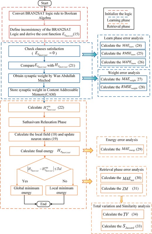
Flowchart of DHNN–BR2SAT.
6 Results and discussion
The purpose of this section is to analyse the effect of the number of redundant second-order clauses
Different cases for the BR2SAT model.
| Case | Model | Proportion |
|---|---|---|
| Case I | BRAN2SAT | |
| Case II | BRAN2SAT. | |
| Case III | BRAN2SAT |
| Case | Model | Proportion |
|---|---|---|
| Case I | BRAN2SAT | |
| Case II | BRAN2SAT. | |
| Case III | BRAN2SAT |
Different cases for the BR2SAT model.
| Case | Model | Proportion |
|---|---|---|
| Case I | BRAN2SAT | |
| Case II | BRAN2SAT. | |
| Case III | BRAN2SAT |
| Case | Model | Proportion |
|---|---|---|
| Case I | BRAN2SAT | |
| Case II | BRAN2SAT. | |
| Case III | BRAN2SAT |
Table 5 presents three different cases for the BRAN2SAT. In Case I, the number of clauses for all three types is generated randomly. In Case II, the proportion of redundant second-order clauses (
6.1 Learning phase
The goal of this phase is to evaluate the learning capability of BRAN2SAT with varying clause proportions within the DHNN framework. During the learning process, these models are embedded into DHNN, and an ES algorithm (Schuurmans & Southey 2001) is employed to achieve a consistent interpretation of BRAN2SAT, thereby establishing the correct synaptic weights for DHNN. Figures 3–5 and Tables 6–8 present the results for
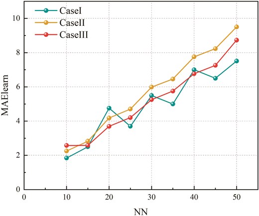
Comparison of
| NN | Case I | Case II | Case III |
|---|---|---|---|
| 10 | 1.8438 | 2.2548 | 2.5785 |
| 15 | 2.5026 | 2.8258 | 2.5823 |
| 20 | 4.7599 | 4.1811 | 3.6932 |
| 25 | 3.6980 | 4.7052 | 4.2056 |
| 30 | 5.4970 | 5.9893 | 5.2526 |
| 35 | 4.9980 | 6.4575 | 5.7542 |
| 40 | 7.0016 | 7.7565 | 6.7696 |
| 45 | 6.5021 | 8.2334 | 7.2596 |
| 50 | 7.5108 | 9.5030 | 8.7298 |
| Best | 1.8438 | 2.2548 | 2.5785 |
| Worst | 7.5108 | 9.5030 | 8.7298 |
| Avg. | 4.9238 | 5.7674 | 5.2028 |
| Avg rank | 1.4444 | 2.7778 | 1.7778 |
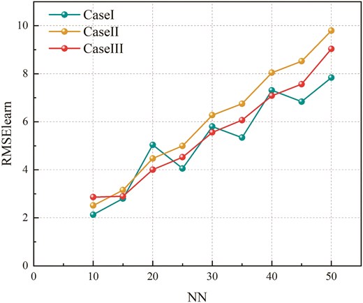
Comparison of
| NN | Case I | Case II | Case III |
|---|---|---|---|
| 10 | 2.1325 | 2.5138 | 2.8634 |
| 15 | 2.8037 | 3.1551 | 2.8990 |
| 20 | 5.0393 | 4.4737 | 4.0061 |
| 25 | 4.0555 | 4.9960 | 4.5252 |
| 30 | 5.8030 | 6.2739 | 5.5597 |
| 35 | 5.3398 | 6.7499 | 6.0670 |
| 40 | 7.3122 | 8.0417 | 7.0842 |
| 45 | 6.8389 | 8.5233 | 7.5660 |
| 50 | 7.8369 | 9.7908 | 9.0329 |
| Best | 2.1325 | 2.5138 | 2.8634 |
| Worst | 7.8369 | 9.7908 | 9.0329 |
| Avg. | 5.2402 | 6.0576 | 5.5115 |
| Avg rank | 1.4444 | 2.7778 | 1.7778 |
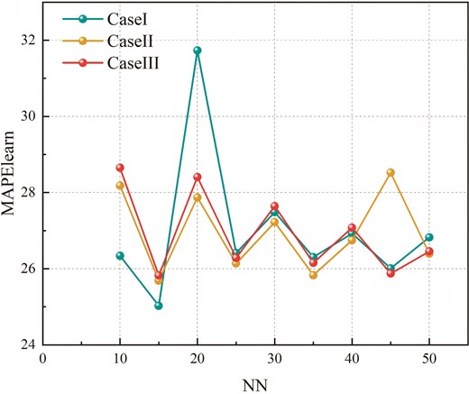
Comparison of
| NN | Case I | Case II | Case III |
|---|---|---|---|
| 10 | 26.3399 | 28.1845 | 28.6499 |
| 15 | 25.0258 | 25.6889 | 25.8234 |
| 20 | 31.7327 | 27.8742 | 28.4091 |
| 25 | 26.4140 | 26.1402 | 26.2851 |
| 30 | 27.4852 | 27.2243 | 27.6451 |
| 35 | 26.3054 | 25.8300 | 26.1555 |
| 40 | 26.9291 | 26.7467 | 27.0784 |
| 45 | 26.0082 | 28.5233 | 25.8750 |
| 50 | 26.8244 | 26.3972 | 26.4538 |
| Best | 25.0258 | 25.6889 | 25.8234 |
| Worst | 31.7327 | 28.5233 | 28.6499 |
| Avg. | 27.0072 | 26.9566 | 26.9306 |
Friedman rank tests are conducted on
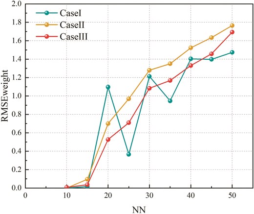
Figures 6 and 7 and Tables 9 and 10 illustrate the
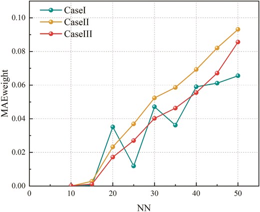
Comparison of
| NN | Case I | Case II | Case III |
|---|---|---|---|
| 10 | 0.0000 | 0.0000 | 0.0002 |
| 15 | 0.0005 | 0.0028 | 0.0011 |
| 20 | 0.0351 | 0.0233 | 0.0172 |
| 25 | 0.0119 | 0.0369 | 0.0271 |
| 30 | 0.0471 | 0.0534 | 0.0402 |
| 35 | 0.0362 | 0.0586 | 0.0463 |
| 40 | 0.0590 | 0.0693 | 0.0555 |
| 45 | 0.0612 | 0.0821 | 0.0671 |
| 50 | 0.0656 | 0.0931 | 0.0856 |
| Best | 0.0000 | 0.0000 | 0.000186 |
| Worst | 0.0656 | 0.0931 | 0.0856 |
| Avg. | 4.9238 | 5.7674 | 5.2028 |
| Avg rank | 1.5000 | 2.7222 | 1.7778 |
Comparison of
| NN | Case I | Case II | Case III |
|---|---|---|---|
| 10 | 0.0000 | 0.0000 | 0.0079 |
| 15 | 0.0161 | 0.0959 | 0.0362 |
| 20 | 1.0967 | 0.6998 | 0.5267 |
| 25 | 0.3659 | 0.9696 | 0.7095 |
| 30 | 1.2127 | 1.2797 | 1.0839 |
| 35 | 0.9469 | 1.3505 | 1.1678 |
| 40 | 1.4036 | 1.5234 | 1.3303 |
| 45 | 1.3979 | 1.6341 | 1.4572 |
| 50 | 1.4736 | 1.7652 | 1.6931 |
| Best | 0.0000 | 0.0000 | 0.0079385 |
| Worst | 1.4736 | 1.7652 | 1.6931 |
| Avg. | 0.8793 | 1.0354 | 0.8903 |
| Avg rank | 1.5000 | 2.7222 | 1.7778 |
Friedman rank tests are conducted on
6.2 Retrieval phase
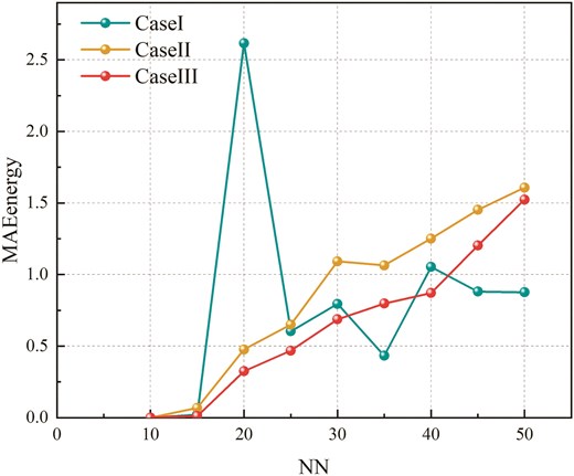
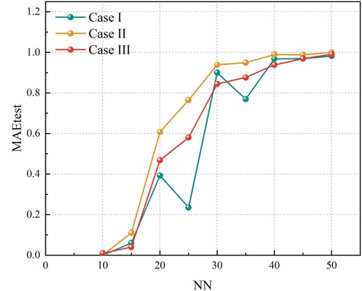
After the DHNN–BR2SAT completes the retrieval of logical consistency during the learning phase, optimal synaptic weights are obtained using the WA method (Abdullah 1992) and stored in the CAM. The model then enters the retrieval phase, where its task is to restore random input neuron states to their stored states. The network automatically adjusts the neuron states based on the input until it reaches a stable state. However, due to the tendency of DHNN to generate repetitive states, output overfitting can occur. Therefore, it is necessary to evaluate the performance of the retrieval phase of DHNN–BR2SAT by assessing energy error, retrieval error, and the quality of global minima (Zamri et al. 2022). Figures 8–10 and Tables 11–13 present the
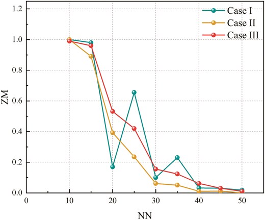
Comparison of
| NN | Case I | Case II | Case III |
|---|---|---|---|
| 10 | 1.0000 | 1.0000 | 0.9900 |
| 15 | 0.9800 | 0.8905 | 0.9600 |
| 20 | 0.1700 | 0.3928 | 0.5317 |
| 25 | 0.6549 | 0.2352 | 0.4200 |
| 30 | 0.1002 | 0.0617 | 0.1557 |
| 35 | 0.2306 | 0.0509 | 0.1239 |
| 40 | 0.0324 | 0.0109 | 0.0619 |
| 45 | 0.0307 | 0.0117 | 0.0307 |
| 50 | 0.018 | 0.0004 | 0.0101 |
| Best | 1.0000 | 1.0000 | 0.9900 |
| Worst | 0.0180 | 0.0004 | 0.0101 |
| Avg. | 0.3574 | 0.2949 | 0.3649 |
| Avg rank | 1.5556 | 2.7222 | 1.7222 |
Comparison of
| NN | Case I | Case II | Case III |
|---|---|---|---|
| 10 | 0.0000 | 0.0000 | 0.0012 |
| 15 | 0.0216 | 0.0683 | 0.0119 |
| 20 | 2.6168 | 0.4771 | 0.3247 |
| 25 | 0.6036 | 0.6510 | 0.4685 |
| 30 | 0.7955 | 1.0925 | 0.6876 |
| 35 | 0.4334 | 1.0642 | 0.7973 |
| 40 | 1.0538 | 1.2515 | 0.8717 |
| 45 | 0.8815 | 1.4521 | 1.2029 |
| 50 | 0.8761 | 1.6077 | 1.5236 |
| Best | 0.0000 | 0.0000 | 0.0012 |
| Worst | 2.6168 | 1.6077 | 1.5236 |
| Avg. | 0.8091 | 0.8516 | 0.6544 |
| Avg rank | 1.7222 | 2.7222 | 1.5556 |
Comparison of
| NN | Case I | Case II | Case III |
|---|---|---|---|
| 10 | 0.0000 | 0.0000 | 0.0100 |
| 15 | 0.0200 | 0.1095 | 0.0400 |
| 20 | 0.8300 | 0.6072 | 0.4683 |
| 25 | 0.3451 | 0.7648 | 0.5800 |
| 30 | 0.8998 | 0.9383 | 0.8443 |
| 35 | 0.7694 | 0.9491 | 0.8761 |
| 40 | 0.9676 | 0.9891 | 0.9381 |
| 45 | 0.9693 | 0.9883 | 0.9693 |
| 50 | 0.982 | 0.9996 | 0.9899 |
| Best | 0.0000 | 0.0000 | 0.0100 |
| Worst | 0.9820 | 0.9996 | 0.9899 |
| Avg. | 0.6426 | 0.7051 | 0.6351 |
| Avg rank | 1.5556 | 2.7222 | 1.7222 |
Further examination of
Friedman rank tests are conducted on
6.3 Total variation and similarity analysis
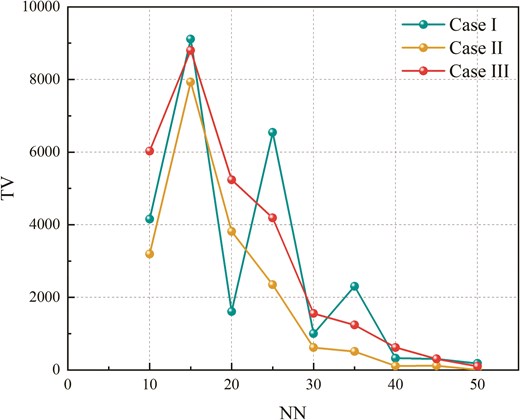
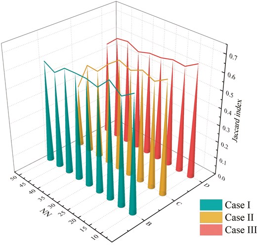
Previous metrics primarily assessed the quantity of DHNN–BR2SAT neuron states, but evaluating the quality of final neuron states is equally essential. This study uses the
S
Comparison of
| NN | Case I | Case II | Case III |
|---|---|---|---|
| 10 | 4153 | 3191 | 6030 |
| 15 | 9114 | 7931 | 8804 |
| 20 | 1610 | 3818 | 5238 |
| 25 | 6542 | 2350 | 4188 |
| 30 | 1002 | 617 | 1556 |
| 35 | 2306 | 509 | 1239 |
| 40 | 324 | 109 | 619 |
| 45 | 307 | 117 | 307 |
| 50 | 180 | 4 | 101 |
| Best | 9114 | 7931 | 8804 |
| Worst | 180 | 4 | 101 |
| Avg. | 2837.6000 | 2071.8000 | 3120.2000 |
| Avg rank | 1.6111 | 2.8889 | 1.5000 |
Comparison of
| NN | Case I | Case II | Case III |
|---|---|---|---|
| 10 | 0.6689 | 0.6571 | 0.6583 |
| 15 | 0.6225 | 0.6152 | 0.6157 |
| 20 | 0.6735 | 0.6437 | 0.6226 |
| 25 | 0.6045 | 0.6132 | 0.6049 |
| 30 | 0.6194 | 0.6393 | 0.6023 |
| 35 | 0.6180 | 0.5878 | 0.5827 |
| 40 | 0.6136 | 0.5182 | 0.6142 |
| 45 | 0.5607 | 0.5227 | 0.6052 |
| 50 | 0.5943 | 0.3643 | 0.5454 |
| Best | 0.5607 | 0.3643 | 0.5454 |
| Worst | 0.6735 | 0.6571 | 0.6583 |
| Avg. | 0.6195 | 0.5735 | 0.6057 |
| Avg rank | 2.4444 | 1.6667 | 1.8889 |
Friedman rank tests are conducted on
6.4 Qualitative analysis of DHNN–BR2SAT
Table 16 presents a qualitative analysis of the DHNN–BR2SAT model under different clause proportions. Based on prior results, it is inferred that Case I achieves optimal performance in both the learning and retrieval stages. Notably, ‘
Qualitative analysis of different DHNN–BR2SAT models.
| NN | Case I | Case II | Case III |
|---|---|---|---|
| NN | Case I | Case II | Case III |
|---|---|---|---|
Qualitative analysis of different DHNN–BR2SAT models.
| NN | Case I | Case II | Case III |
|---|---|---|---|
| NN | Case I | Case II | Case III |
|---|---|---|---|
6.5 The limitation of DHNN–BR2SAT
Through the above analysis, we have gained a comprehensive understanding of the distributions of learning error, synaptic weight error, energy, final solutions, neuron variations, and similarity indices, which has allowed for a systematic evaluation of the overall behaviour of DHNN–BR2SAT. The results indicate that embedding BRAN2SAT within DHNN facilitates obtaining ideal global minima and achieving diverse neuron states. However, based on the no free lunch theorem (Wolpert & Macready 1997), we conclude that no single model is optimal for all scenarios, as each model produces unique outcomes. This study is limited by computational time. The presence of redundant variables doubles the number of clauses, making it challenging for the model to find the correct interpretation during the learning phase. With larger
7 Conclusion
This study introduces a novel logical rule, termed BRAN2SAT, consisting of redundant second-order clauses and non-redundant first- and second-order clauses. The logical rule is implemented into DHNN by minimizing the cost function of the network, forming DHNN–BR2SAT. During the learning phase, the optimal synaptic weights are computed by comparing the cost function with the energy function. In the retrieval phase, the network achieves a stable state by updating fewer neurons. The effectiveness of the DHNN–BR2SAT model is evaluated by varying the proportions of different clause orders, with performance evaluated using various metrics during both the learning and retrieval phases. Experimental results indicate that when the numbers of the three types of clauses are randomly selected, the DHNN–BR2SAT model achieves optimal performance. Notably, this is the first attempt to implement logic containing redundant literals into DHNN, highlighting the potential of this approach to improve model performance when dealing with overlapping data.
Future directions. Metaheuristic algorithms are employed to optimize the retrieval phase, facilitating the generation of a more diverse final solution. Furthermore, the DHNN–BR2SAT model offers a novel approach to logic mining, with potential applications in practical problems such as sentiment analysis, industrial data classification, and financial investment forecasting. The DHNN–BR2SAT model represents a significant advancement in logic mining, filling the gap in extracting overlapping knowledge, and offering substantial potential for applications in various domains.
Conflicts of Interest
The authors declare that they have no known competing financial interests or personal relationships that could have appeared to influence the work reported in this paper.
Author Contributions
Binbin Yang: Methodology, Writing – original draft, Writing – review & editing. Guoxiang Li: Project administration, Data curation. Adila Aida Azahar: Writing – review & editing, Data curation. Mohd Shareduwan Mohd Kasihmuddin: Supervision, Methodology. Yuan Gao: Methodology, Data curation. Suad Abdeen: Writing – review & editing, Methodology. Baorong Yu: Visualization, Writing - review & editing.
Funding
The authors are grateful for the financial support from the National Natural Science Foundation of China (no. 62162006). Additionally, we acknowledge the support by Guangxi Key Laboratory of Big Data in Finance and Economics Project Fund, Guangxi First-class Discipline statistics Construction Project Fund and Guangxi University Young and Middle-aged Teachers’ Research Capacity Enhancement Project (nos 2021KY0907, 2021KY0378, and 2023KY1293) and Guangxi Key Laboratory of Seaward Economic Intelligent System Analysis and Decision-making (no. 2024C013).
Data Availability
No data were used for the research described in the article.
Acknowledgments
The authors would like to thank the anonymous referees for their valuable comments and suggestions.
References
Author notes
These two authors contributed equally to this work.
