


Abstract
In many practical and academic contexts, the demand for dynamically expanding data attributes in machine learning models has become increasingly prominent. As data evolves due to continuous collection and new discoveries, models often need to incorporate new feature dimensions without requiring complete retraining. Incremental Attribute Learning (IAL) is designed to address this challenge by progressively integrating new features while preserving the model’s performance on previously learned data. Our method combines an innovative embedding layer algorithm to handle dynamically changing input dimensions and a knowledge distillation strategy to retain essential information from prior model states. The redesigned loss function utilizes soft labels generated from earlier outputs, minimizing the divergence between the new model’s predictions and the original model’s behavior. This approach ensures stable performance on previously learned attributes while effectively incorporating new features. Extensive experiments across 11 tabular datasets, covering binary classification, multi-class classification, and regression tasks, indicate that our approach surpasses traditional incremental attribute learning methods and conventional retraining in terms of accuracy and efficiency. Compared to existing incremental attribute learning models, our model requires only a fraction of the training time and achieves a relative improvement of 7.97% in classification tasks. Furthermore, our approach exhibits minimal forgetfulness of old format data, with a forgetting rate of ∼1% per increment stage, while maintaining strong performance on new format data. In conclusion, this research presents a novel approach to IAL that effectively combines knowledge distillation and a specialized feature transformation layer. Given that the current model is primarily focused on tabular data, future research should prioritize extending this framework to more complex data types and optimizing memory efficiency. Additionally, refining soft label selection and exploring more efficient embedding strategies is expected to improve the adaptability and scalability of IAL in broader applications.
Reevaluated incremental attribute learning with complex data.
Introduced a feature transformation module to manage the unpredictability of input dimensions.
Introduced distillation algorithms to solve catastrophic forgetting.
Improve performance on new data with minimal forgetfulness on old data.
Experiments conducted on datasets from 11 different fields demonstrate the versatility.
1. Introduction
Neural networks can be used to learn nonlinear mappings between the input space and the output space with a set of parameters. During the traditional learning phase, the networks are basically assumed to exist in a static environment, the dimension of the input space is fixed; the training process of the model is an iteration over the entirety of the dataset.
However, as shown in Fig. 1, in practical applications, both the dataset and the network often need to be dynamically updated. We need to learn from new data as they become available, and continuously update its model parameters in response to newly arrived samples incrementally (Gepperth & Hammer, 2016; Fang & Liu, 2021). This approach is particularly useful in scenarios where data continuously arrive from a data stream and there is a need to adapt to changing environments (Lemzin, 2023).

Comparing general incremental learning with IAL.
Current mainstream research on incremental learning primarily addresses areas such as task-incremental, domain-incremental, and class-incremental learning (van de Ven et al., 2022). In these incremental approaches, although the nature of the data (tasks, domains, classes) may vary, the fundamental structure (e.g., input dimensions) remains consistent. Unlike these general incremental learning methods, which maintain a consistent input structure, incremental attribute learning (IAL) requires the model to accommodate new features, potentially altering the input dimensions. As shown in Fig. 1, this approach emphasizes adapting to new attributes or features, as effectively utilizing all features plays a crucial role in determining the upper bound of model performance (Lee, 2023).
In practical applications of models, there are many scenarios suitable for IAL. After deploying a model, the dataset may continuously update, and new feature dimensions may be added. This can occur due to new data sources, additional sensors, different sampling rates, or other external factors. For example, as shown in Fig. 2, Xu et al. (2020) noted that some features in e-commerce recommendation system models can only be observed after a user clicks on an item and cannot be observed during the initial model training stage. Sometimes, models are required to extract features directly from unprocessed data dynamically. This extraction process, facilitated by specific algorithms or procedural steps, might result in the emergence of novel feature dimensions. In such scenarios, the dimensionality and distinct characteristics of the forthcoming features remain entirely unknown before their emergence, necessitating that the model can accommodate these novel feature dimensions.
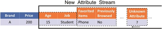
Incremental Attribute Integration in E-commerce Data Streams
For example, an e-commerce recommendation system may initially only include product information. After the platform goes live, user information can be incrementally added. As users interact with the system, their behavior data are collected. In the future, additional useful features may be integrated into the recommendation system. This process is iterative and progressive. Initially, the developers of the recommendation system may not be aware of which information will become new features in the future.
To address this issue, Guan & Li (2001) first proposed a method that utilizes neural networks, referred to as “Incremental Learning in terms of Input Attributes” (ILIA), to train separate sub-networks for each input attribute. Numerous existing studies have also endeavored to integrate IAL with techniques such as feature selection, k-nearest neighbor, and others, aiming to tackle specific challenges like object detection (Wang et al., 2018) and credit card fraud detection (Sadreddin & Sadaoui, 2022). However, despite the significant advancements made by neural networks in recent years, there is still very little work that proposes new networks different from ILIA, exploring new foundational models and training paradigms in the field of IAL.
In this work, we introduce a novel paradigm for IAL, leveraging methodologies inspired by self-distillation and cross-modal distillation. By redesigning the loss function and embedding layer algorithm specifically for incremental learning, this paradigm effectively tackles two major challenges: the catastrophic forgetting problem in the incremental process and the unpredictability of input dimensions. We constructed 11 tabular datasets with different tasks, including binary classification, multi-class classification, and regression, and conducted tests on these datasets. Through extensive testing, we found that our method outperforms both retraining a new model and using the original model on the incremental datasets while maintaining consistency with the output of the original model. This method comprehensively surpasses the currently used ILIA algorithm in terms of both time and performance. The algorithm source code is publicly available at https://github.com/kuirh/IAL-KD.
Compared to existing works, to the best of our knowledge, we are the first to redesign a deep neural network specifically for the IAL problem. Our work’s characteristics are summarized as follows:
We have reevaluated the task of IAL and expanded the scope of attribute increments to more complex tabular data formats using deep learning techniques.
We have designed a feature transformation module and distillation algorithms for IAL, addressing the challenges of catastrophic forgetting and the unpredictability of input dimensions for incremental learning across different input formats.
Through experiments on 11 dataIAL models, our model requires only a fraction of the training time needed by current methods. It also achieves a relative improvement of 7.97% in classification tasks over the existing IAL method. Our approach not only maintains superior performance on new format data but also exhibits minimal forgetfulness of previously learned formats.
2. Related work
2.1 Incremental learning
Incremental learning is a machine learning paradigm where the model is trained continuously as new data become available, rather than training on a fixed dataset all at once (Gepperth & Hammer, 2016).
The existing methods in incremental learning can be mainly divided into three categories. The first category focuses on dynamically expanding the network structure to accommodate new tasks during the learning process (Rusu et al., 2016; Li et al., 2019; Peng et al., 2023). For example, Rusu et al. (2016) add new neural network columns for each new task while preserving and leveraging previously learned features via lateral connections. However, for long-term incremental learning, the linear growth of parameters makes continuously expanding the network structure impractical.
The second category involves replaying previous tasks’ data stored in a memory to mitigate forgetting. Recent studies have explored different approaches to exemplar replay, such as storing class centroids as prototypes and augmenting them with Gaussian noise to create synthetic data for replay (Lin et al., 2022; Zhang & Gu, 2023).
The third category is regularization. One form of regularization involves constraining model parameters to prevent drastic changes during training. Techniques like elastic weight consolidation (EWC) add a penalty to the loss function based on the importance of the weights to previous tasks (Hyder et al., 2022; Gok et al., 2023; Thakur et al., 2022). Another form is knowledge distillation (KD), which was first introduced in Li & Hoiem (2017) and subsequently applied and extended more broadly. For instance, it has been combined with representation learning in Rebuffi et al. (2017), linked with example selection in Kang et al. (2022), and utilized for automatically selecting the hyperparameters for the extent of model updates in Liu et al. (2023). The core of this technique lies in intuitively reducing the forgetting of old class knowledge by ensuring the consistency of outputs between the new and old models on given data.
Due to the effectiveness of distillation-based methods, this paper attempts to extend the distillation-based approach from other incremental learning domains to IAL.
2.2 Incremental attribute learning
The concept of IAL was first proposed by Guan & Li (2001), who used neural networks to train sub-networks for each input attribute separately and then combined them as the final solution. As Fig. 3 shows, this approach avoids redesigning the entire network and enables incremental learning of new attributes.
Current approaches to IAL: the ILIA network.
In recent years, there have been advancements in combining IAL with feature preprocessing techniques such as feature extraction, selection, and ordering (Gepperth & Hammer, 2016; Wang et al., 2016). These techniques have shown improved classification performance. Gepperth & Hammer (2016) and Wang et al. (2015) provided mathematical analysis on why IAL can outperform conventional batch training methods and proved the importance of feature ordering for IAL’s performance gain. Sadreddin & Sadaoui (2021) further enhanced the process by introducing a dynamic neural network construction that adapts to the inclusion of new feature groups. Additionally, the integration of IAL with algorithms like k-nearest neighbors has resulted in fast and effective pattern classification (Wang et al., 2018). Silvestrin et al. (2023) propose a transfer learning algorithm for linear regression that combines historical data with newly collected data, which have different input dimensions.
In terms of specific applications, Wang et al. (2014) proposed a time feature extraction method to address the characteristics of time series data. This method combines original features with temporal state differences to create new second-order features as part of the input for the IAL system. This approach applies IAL to time series classification problems and explores its application in time series data such as electroencephalogram-based eye state recognition. Sadreddin & Sadaoui (2021) introduced a novel incremental learning method for credit card fraud detection. This method not only adapts to new patterns and changes in data streams but also improves model performance and training efficiency while protecting user privacy.
2.3 Knowledge distillation
KD has become a popular technique for transferring knowledge from one model to another (Hinton et al., 2015).
In recent years, numerous advancements in distillation techniques, such as self-distillation and multi-step distillation, have emerged. These methods involve a model distilling knowledge from itself over different training iterations or through a sequential distillation process, where intermediate models act as teachers for subsequent student models. Gou et al. (2023) demonstrated that multi-stage learning with stage-wise distillation is more effective than a single transfer. Zhang et al. (2021) and Xu et al. (2022) showed that a model can learn from its own predictions and use this knowledge to improve its performance.
Recent work has leveraged these distillation techniques to address the issue of forgetting in incremental learning, enabling machine learning models to learn continuously and adaptively without losing previous knowledge. For instance, Yun et al. (2021) demonstrated the potential of correct KD, addressing long-sequence effectiveness degradation in task incremental learning, particularly in 3D object detection, and achieving near upper-bound performance. Dong et al. (2021) expanded on these concepts by introducing an exemplar relation distillation framework for few-shot class incremental learning, balancing the preservation of old knowledge with adaptation to new knowledge. Furthermore, Michieli & Zanuttigh (2021) applied KD to semantic segmentation for incremental learning, proposing methodologies that maintain accuracy on previously learned classes without the need to store images from earlier training stages. Additionally, Liu et al. (2024) and Sun et al. (2024) explored the application of distillation techniques to train a continually learning text-to-image mapping model capable of handling different types of tasks. Their work demonstrates the extensive potential of combining distillation methods with incremental learning techniques across diverse application scenarios.
3. Methodology
This section introduces a novel method called IAL based on KD (IAL-KD). By integrating IAL into the training process, IAL-KD significantly enhances both accuracy and efficiency. In contrast to traditional methods that do not employ IAL, IAL-KD not only improves the precision of the model but also reduces the training time required.
3.1 Problem definition
Our focus is on the training process, while the inference process is performed directly using the latest model |$M_t$| without requiring any additional operations. Drawing on previous research achievements, we define IAL as a process involving the progressive introduction of training data. This process implies that the dimensions of input data available for model learning continually expand at each incremental stage. We concentrate on supervised learning problems, where at each incremental step |$T = \lbrace 1, 2, \ldots , t\rbrace$|, the model is provided with a set of N manually annotated training samples, where N denotes the number of samples. These training samples are denoted as |$D^t = \lbrace X^{1:t}, Y\rbrace = \lbrace x^{1:t}_i, y_i\rbrace _{i=1}^N$|. Here, |$X^{1:t}$| represents the inputs after adding the newly introduced attributes at stage t in incremental learning, while Y represents the true labels that remain unchanged over time.
At the incremental learning process at step t, the model |$M^t$| is updated using the data |$D^t$| following an incremental learning method. In each learning phase, the model may receive |$m^t$| numerical features |$X^t_{\text{num}} \in \mathbb {R}^{m^t}$| and |$c^t$| categorical features |$X^t_{\text{cat}_i}$| with |$k^t_i$| categories each. Our model takes one-hot encoded versions of categorical features as input. That is, if a categorical feature has c categories, then |$X^t_{\text{cat}_i} \in \lbrace 0, 1\rbrace ^{k_i^t}$|.
For each increment of data samples, the input data are represented as |$X^t = \lbrace X^t_{\text{num}}, X^t_{\text{cat}_1}, \ldots , X^t_{\text{cat}_{c^t}}\rbrace$|. Therefore, the incremental dimension of |$X^t$| is |$\left(m^t + \sum _{i=1}^{c^t} k_i^t\right)$|. The entire input sample |$X^{1:t} = \cup _{i=1}^t X^i$|, which includes all the dimensions the model has learned, has a dimensionality of |$l^t= \sum _{j=1}^t \left(m^j + \sum _{i=1}^{c^t} k_i^t\right)$|, along with their corresponding labels Y.
A neural network learner at an incremental stage t, denoted by |$M^t(\cdot )$|, involves a feature transformation module layer |$h(\cdot )$|, C building blocks |$\lbrace f_{c}(\cdot ) ; c=1, 2, \dots , C \rbrace$|, and a task layer |$g(\cdot )$|, which is expressed as
Our primary goal is to optimize the following objective function to ensure that the model performs better after receiving new attributes: |$\min _{M^t} \left[ L(M^t(X^{1:t}), Y) \right]$|. At the same time, we aim to maintain compatibility with the original input format, considering that not all data may have received the new attributes. Therefore, we also optimize the performance on previous input stages: |$\min _{M^t} \sum _{p=1}^{t-1} \left[ L(M^t(X^{1:p}), Y) \right]$|.
The key symbols used to describe our framework are summarized in Table 1 for clarity.
Symbol definitions.
| Symbol | Definition |
|---|---|
| t | Incremental learning stage |
| |$M_t$| | Model at stage t |
| |$D^{1:t}$| | Incremental dataset at stage t |
| |$X^{1:t}$| | Input data after t incremental stages |
| |$X^{t}$| | Newly added incremental attributes at stage t |
| |$l^{t}$| | Dimension of input data after t incremental stages |
| Y | Set of true labels |
| |$\hat{Y}^{t}$| | Predicted labels at stage t |
| |$Y^{t}_\text{soft}$| | Soft labels generated by the output at stage t |
| |$V^t$| | Intermediate representation in the model at stage t |
| |$\tau$| | Temperature controlling the distillation process |
| |$\lambda$| | Weight of the distillation loss |
| |$\alpha$| | Base of the loss decay factor |
3.2 Proposed method
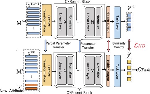
In this work, we propose an incremental learning framework as shown in Fig. 4, which is applicable in scenarios where data are continuously available and the network is capable of lifelong learning. The figure illustrates an example of incremental learning with a single data sample.
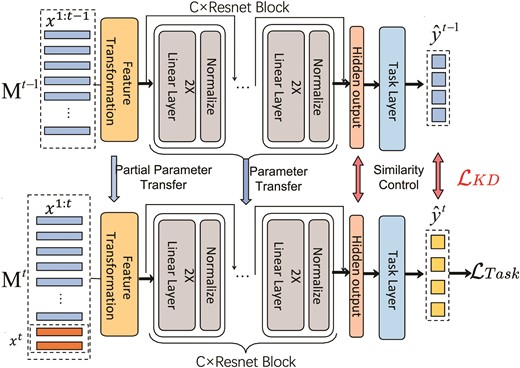
Our IAL-KD method.
3.2.1 Backbone network
We have developed a cross-stage distillation framework by drawing inspiration from KD. This framework is primarily based on the following considerations:
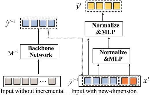
Model |$M_t$| primarily consists of the following components. The transformation module layer |$h^t(\cdot )$| performs feature mapping, where the input |$X^{1:t} \in \mathbb {R}^{l^t}$| varies with stage t, while the output dimension remains fixed at |$\mathbb {R}^{d1}$|. Unlike a regular fully connected layer, which produces an output |$y \in \mathbb {R}^{d1}$| based on |$y = Wx + b$|, this mapping clearly cannot accommodate the variability in the dimension of x. Therefore, for the feature transformation layer, we propose |$y = W^{\prime }x + b$|. We will utilize the feature transformation layer from the previous teacher model and update it incrementally. We calculate the average value of each row of the weight matrix and add this average value vector |$\bar{w} = \frac{1}{l^{t-1}} \sum _{i=1}^{l^{t-1}} W_{:,i}$| as a new column to W. Then, we apply the normalization coefficient |$\text{normt} = \frac{l^{t-1}}{l^t}$|, forming a new weight matrix: |$W^{\prime } = [W \, |\, \bar{w}] \times \text{normt}$|.
In this way, we achieve the following: for the original input features, we continue to use the original linear transformation for initialization, but with rescaling. For the new input features, we initialize the mapping based on the mean of the previous mappings, thereby effectively inheriting the original information, as shown in Fig. 5.
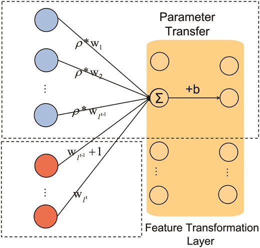
Feature transformation module.
We use ResNet as building blocks |$f_c(x) = x + \operatorname{Drop}(\operatorname{Linear}(\operatorname{Drop}(\operatorname{ReLU}(\operatorname{Linear}(\operatorname{Norm}(x))))))$| due to its demonstrated competitive performance, simplicity, and effectiveness as a baseline for tabular deep learning in previous works (Gorishniy et al., 2021).
The task layer |$g(\cdot )$| maps the embedding vector |$V^t$| given by the last building block to a vector |$\hat{Y}^{t}$| corresponding to the dimensions of Y.
3.2.2 Distillation method
By controlling the distillation loss during the incremental stage t, we ensure that it does not diverge from the previous stage |$M_{t-1}$|. This guarantees that the new incremental model can effectively utilize the feature extraction capabilities of the preceding stage model and facilitates rapid model convergence.
For multi-class classification tasks, we generate soft labels that represent class probabilities as distributions instead of hard labels (e.g., 0 or 1). This method smooths the probability distribution and incorporates additional information, such as model uncertainty and class similarity.
Using the soft labels from the previous stage model |$M^{t-1}$|, the model at stage t can learn more comprehensively from its own outputs. This approach surpasses the limitations of relying solely on hard labels, allowing the model to gain a deeper understanding and effectively improve its performance.
The formula for generating soft labels is as follows. |$\tau$| is the hyperparameter temperature that controls the distillation process.
For regression and binary classification tasks, we utilize the intermediate representations V from the last hidden layer before the task layer |$g(\cdot )$|, similar to the concept of soft labels. These representations offer a more informative foundation for learning, capturing subtle patterns in the data. Using these intermediate features, the incremental model can effectively grasp the underlying data patterns, thus improving its performance.
To facilitate KD, we employ a distillation loss function, denoted as |$L_{KD}$|, which transfers knowledge from a teacher model to a student model, thereby enhancing the performance of the student model. The distillation loss function is designed to measure the divergence between the softened outputs of the teacher and student models. The formula for the distillation loss is as follows:
Here, |$Y^{t}_\text{soft}$| and |$Y^{t-1}_\text{soft}$| represent the soft labels generated by the student model at stage t and the teacher model at stage |$t-1$| for classification tasks. Using the Kullback–Leibler divergence |$L_{\text{KL}}$|, we measure the difference between these two probability distributions. This approach allows the student model to learn not only the final decision but also the distribution of predictions, providing richer information and leading to better generalization. Similarly, for regression tasks, |$V^{t}$| and |$V^{t-1}$| represent the intermediate representations from the last hidden layer before the classifier in the student and teacher models. Using the mean squared error (MSE) loss to measure the differences between these representations, we ensure that the knowledge transfer is effective, as the student model retains and refines the patterns learned by the teacher model.
3.3 Practical loss function
Our goal is to enhance the representational capacity of the new model based on the old one and improve its classification performance on the target task. To achieve this, we design a comprehensive loss function that includes both task-specific loss and distillation loss. The task-specific loss varies according to the type of task. For regression tasks, we use the MSE loss, and for classification tasks, we utilize the cross-entropy loss. This is denoted as |$L_{\text{Task}}$|:
By combining the task-specific loss |$L_{\text{Task}}$| and the distillation loss |$L_{KD}$|, our comprehensive loss function ensures that the new model not only learns effectively from the true task labels but also benefits from the knowledge distilled from the previous model. This approach leads to improved performance and faster convergence of the incremental model.
Cho & Hariharan (2019) suggested that the impact of distillation is not always positive. While KD can aid the student model’s learning process in the early stages of network training, it may hinder further learning in the later stages. To mitigate this issue, we employ a loss decay strategy called Early Decay Teacher (Zhou et al., 2020), which gradually decreases the weight of the distillation loss during training. This approach allows the student model to find its own optimization space. Specifically, we replace the distillation loss weight |$\lambda$| with |$\lambda \times \alpha ^{n_e}$|, where |$n_e$| represents the n-th epoch in the training process.The final loss function is
4. Experiments
This section compares our algorithm with previous methods on 11 different datasets and analyzes the results of ablation studies. Additionally, it investigates the principles underlying the effectiveness of our model.
4.1 Scope of the comparison
In our work, we focus on validating the effectiveness and generality of the proposed feature incremental learning through distillation, aiming to establish it as a universal paradigm.
We accomplish this by conducting experiments on multiple datasets across different deep learning tasks, including multi-class classification, binary classification, regression, and ranking.
We will attempt to demonstrate the superiority of our method by comparing performance metrics, training time, and space requirements with two other approaches that do not employ incremental learning: using the old model directly and retraining the model from scratch.
We will validate the persistence and usability of our method in practical application scenarios by conducting multiple rounds of incremental learning. We will assess the consistency of the output results and evaluate the method’s performance.
We will explore the performance of old data formats on a new model and compare its performance with the previous incremental attribute algorithm. Additionally, we will evaluate the model’s performance maintenance based on the forgetting rate (FR).
We conduct extensive ablation studies to investigate the effectiveness of each module, including replacing or removing components and verifying the robustness of distillation-related hyperparameters. We perform thorough comparative experiments to demonstrate the effectiveness of our method, including comparisons with the specially designed neural network “ILIA” method and other regularization methods that do not use distillation, such as those using the Fisher Information Matrix (FIM).
4.2 Dataset and data preprocessing
We refer to the methodology described in Gorishniy et al. (2021) for constructing the datasets. We use an extensive collection of 11 public datasets. Each dataset is meticulously divided into train-validation-test splits to ensure consistent use across all algorithms. These datasets encompass various problem types, including single-classification, multi-classification, and regression. They cover a wide range of domains, including California Housing (Kelley Pace & Barry, 1997) for real estate data, Adult (Kohavi, 1996) for income estimation, Helena (Guyon et al., 2019) and Jannis (Guyon et al., 2019)) for anonymized datasets, Higgs Small (Baldi et al., 2014) for simulated physical particles (using the version with 98K samples from the OpenML repository), ALOI (Geusebroek et al., 2005) for images, Epsilon (Everingham et al., ????) for simulated physics experiments, Year for audio features, Covertype (Blackard & Dean, 2000) for forest characteristics, and Yahoo (Chapelle & Chang, 2011) and Microsoft (Qin & Liu, 2013) for search queries. For ranking problems such as Microsoft and Yahoo, we adopt the pointwise approach to learning-to-rank and treat them as regression problems. Details of the datasets can be found in Table 2.
Dataset information.
| Name | Objects | Num | Cat | Task type |
|---|---|---|---|---|
| Cal Housing | 20640 | 8 | 0 | Regression |
| Adult | 48842 | 6 | 8 | Binclass |
| Helena | 65196 | 27 | 0 | Multiclass |
| Jannis | 83733 | 54 | 0 | Multiclass |
| Higgs Small | 98050 | 28 | 0 | Binclass |
| ALOI | 107000 | 128 | 0 | Multiclass |
| Epsilon | 500000 | 2000 | 0 | Binclass |
| Year | 516345 | 90 | 0 | Regression |
| Covtype | 581012 | 54 | 0 | Multiclass |
| Yahoo | 709877 | 699 | 0 | Regression |
| Microsoft | 1207192 | 136 | 0 | Regression |
4.3 Evaluation metrics
In the domain of neural network learning, diverse metrics of performance are employed to assess distinct categories of problems. For instances of regression problems, such as California Housing, Year, Yahoo, and Microsoft, where the task lies in forecasting continuous values (e.g., housing prices, temperatures), and our primary focus is on quantifying the level of dissimilarity between the predicted and actual values, the evaluation metric employed is root mean square error (RMSE).
For classification problems such as Adult, Helena, Jannis, ALOI, Epsilon, and Covertype, where the model must predict discrete categories (e.g., spam or not, disease diagnosis), our primary concern is the proportion of correctly classified samples. Therefore, the evaluation metric employed is accuracy. Additionally, we have uploaded precision, recall, and F1-score metrics from the training process to the code repository to provide a comprehensive assessment of the model’s performance.
The FR is a metric used to evaluate the degradation in a model’s performance after it has been updated with new data. It is particularly relevant in incremental learning scenarios where the model must adapt to new information without losing the knowledge it has already acquired. The FR is calculated as the difference between the model’s performance before and after the update, normalized by the initial performance. A high FR indicates significant performance loss, while a low rate suggests the model retains its knowledge effectively. The FR is calculated as
where |$P_{\text{before}}$| represents the performance metric before the update, and |$P_{\text{after}}$| represents the performance metric after the update. P are designed so that higher values indicate better performance (accuracy for classification or negative RMSE for regression, for consistency).
By measuring the similarity between the model’s outputs before and after learning new tasks or data, |$\hat{Y}^{t-1}$| (before) and |$\hat{Y}^{t}$| (after), we can evaluate how well the model is incrementally incorporating new knowledge. High similarity may suggest that the model is effectively building upon its previous understanding. Maintaining high consistency across the incremental learning process can potentially reduce forgetting in continual learning scenarios (Bhat et al., 2022).
Similarity, which ranges from 0 to 1, is based on the Euclidean distance between the model’s outputs. To ensure the outputs are comparable and scaled between 0 and 1, we normalize the outputs |$\hat{Y}^{t}$| and |$\hat{Y}^{t-1}$|. This normalization process adjusts the magnitude of the vectors, placing them on a common scale. The similarity can be computed using the following formula:
4.4 Implementation details
4.4.1 Data preprocessing
The preprocessing of data is a critical step in our IAL-KD framework. It involves generating the incremental dataset |$D^{1:t}$|, which is used to update the model at each stage of incremental learning. Due to the lack of readily available datasets specifically designed for IAL tasks, we simulate the scenario where attributes are introduced incrementally by adopting a strategy that involves masking out columns from conventional datasets. The process is as follows:
Initially, we randomly remove columns from the dataset to create a version without incremental attributes. This represents the initial state of the dataset at the beginning of the learning process, where the model is trained on a fixed set of attributes.
At each subsequent stage |$t = 2, 3, \ldots , T$|, new data are incrementally added to the dataset. Formally, this is represented as |$D^{1:t} = D^{1:t-1} \cup D^{t}$|, where |$D^{t}$| includes the columns that were previously masked. This step-by-step reintroduction of columns simulates the addition of new attributes.
These preprocessing steps, including the removal and reintroduction of columns, are completely invisible to the model. By employing this strategy, we ensure that the model is exposed to an incremental learning environment, enabling it to progressively learn and adapt to new attributes.
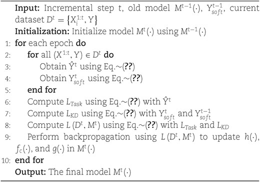
4.4.2 Algorithm
The following pseudocode describes the algorithm for performing a single data increment, which is fundamental to incremental attribute algorithms. Using classification tasks as an example, we start by feeding data into the existing model and calculating the soft labels according to equation (2). During the next training session, these soft labels are compared with those produced by forward propagation of the new format data in the new model, serving as the distillation loss. This distillation loss is combined with the task loss, which arises from the forward propagation of the new format data, to compute the overall loss for backpropagation. For regression tasks, we replace the task loss function accordingly and use the features V before entering the classification layer instead of soft labels. If multiple increments are needed, the algorithm shown in Algorithm 1 should be executed multiple times.
Train the model for time step t
4.4.3 Benchmark setting
To evaluate the effectiveness of our IAL-KD approach, we have established a comprehensive benchmarking framework. This setup allows us to systematically compare different models and methodologies, providing a fair and thorough assessment. By comparing direct retraining and incremental learning without distillation, we can accurately measure the benefits of our approach in terms of knowledge retention, performance improvement, and training efficiency. The training and inference of our deep learning models were executed on a high-performance server equipped with NVIDIA 3090 GPU.
Old model: We first train a model on the old dataset, which does not include the new incremental attributes. This model serves as the knowledge source for the distillation process in our IAL approach.
Retraining: We retrain a model from scratch on the combined dataset, which includes both the initial data and the new incremental data. This model serves as a baseline to compare the performance of our IAL method.
ILIA model (Guan & Li, 2001): The ILIA network architecture is implemented through a modular design. Each module in the network is dedicated to learning a specific subset of input features. As new data become available, additional modules are introduced to handle these new features, while existing modules continue to operate on the previously learned features.
IAL with EWC: We use EWC to preserve important information from previous stages of training. EWC employs the FIM to estimate the importance of model parameters for previously learned tasks and incorporates a regularization term in the loss function to penalize changes to these important parameters. This approach helps maintain the model’s performance on earlier tasks while learning new attributes (Gepperth & Wiech, 2019).
IAL with KD: Our IAL-KD model is updated incrementally with each new dataset. The model leverages the KD process to transfer knowledge from the old model, ensuring that the new model retains the knowledge acquired from previous data.
4.4.4 Model hyperparameters configuration
The hyperparameters for our IAL-KD model are carefully selected to optimize performance and facilitate efficient learning. The configuration is based on the ResNet architecture, with specific parameters detailed below:
Feature transformation module: The feature transformation function |$g(\cdot )$| maps input X of various dimensions to a uniform dimension of 348.
Backbone Resnet configuration: The building blocks |$f_c$| consist of an eight-layer ResNet. The hidden layer dimension in the residual block is set to 339, which determines the size of the fully connected layer within the residual block. The training batch size is set to 512, while the evaluation batch size is 128. The learning rate is initialized at 0.001, and the model is trained for 50 epochs. The optimizer used is AdamW, which combines the benefits of Adam and weight decay. Early stopping is implemented with a patience of 12 epochs, selecting the best-performing model on the validation set as the final test model.
Distillation: A temperature of 3 is used in the distillation process to control the softness of the softmax output. The learning rate decay factor (|$\alpha$|) is set to 0.9, and the distillation loss weight decay factor (|$\alpha _{\text{decay}}$|) is set to 0.95. These decay factors are used to gradually reduce the influence of the teacher model as the student model becomes more confident.
5. Results
This section presents the experimental results of our IAL approach using KD. The performance of our method is compared with direct retraining and incremental learning without distillation on a variety of datasets. The datasets include both classification and regression tasks, ensuring a comprehensive evaluation of our proposed method.
5.1 Main results
We conducted a comparative analysis within the context of a single incremental stage to assess whether our IAL-KD model has advantages in terms of time and performance compared to training a new model from scratch. Additionally, we examined whether the introduction of new data features in the IAL-KD model |$M^t$| leads to better performance compared to the old model |$M^{t-1}$|, which only utilizes the original data features. Using the 11 datasets mentioned earlier, we carried out 30 to 100 repeated incremental experiments on each dataset, varying the number according to the complexity involved. We averaged the results of these experiments and detailed the comparative outcomes in Table 3.
Benchmark scores on 11 different datasets.
| Our IAL-KD | IAL-KD (early stop) | Old Model | Retraining | |||||||||
|---|---|---|---|---|---|---|---|---|---|---|---|---|
| Classification | Epoch | Time(s) | Accuracy | Epoch | Time(s) | Accuracy | Epoch | Time(s) | Accuracy | Epoch | Time(s) | Accuracy |
| Adult | 25.55 | 35.41 | 85.53% | 5 | 10.18 | 85.54%† | 24.14 | 33.84 | 85.01% | 23.64 | 32.35 | 85.51% |
| Higgs Small | 21.19 | 88.59 | 72.09%† | 5 | 30.24 | 71.75% | 32.94 | 90.15 | 71.84% | 30.42 | 95.53 | 71.97% |
| EPSILON | 24.27 | 326.08 | 89.45% | 5 | 73.90 | 89.46%† | 26.52 | 338.43 | 89.45% | 27.23 | 335.55 | 89.45% |
| Helena | 19.66 | 23.23 | 37.48% | 5 | 5.78 | 37.34% | 27.59 | 35.55 | 37.49%† | 22.91 | 36.97 | 36.28% |
| Jannis | 59.14 | 67.11 | 71.74%† | 5 | 8.77 | 70.64% | 60.45 | 63.37 | 71.55% | 60.41 | 62.40 | 71.62% |
| ALOI | 22.25 | 195.38 | 96.03% | 5 | 57.76 | 96.62%† | 43.16 | 357.17 | 94.29% | 43.49 | 384.29 | 94.96% |
| Covtype | 121.24 | 2429 | 96.30%† | 5 | 227.70 | 90.08% | 122.56 | 2402 | 96.23% | 122.42 | 2433 | 96.29% |
| CLS_AVG | 41.9 | 452.11 | 78.37%† | 5 | 59.19 | 77.35% | 48.19 | 474.36 | 77.98% | 47.22 | 482.87 | 78.01% |
| Regression | Epoch | Time(s) | RMSE | Epoch | Time(s) | RMSE | Epoch | Time(s) | RMSE | Epoch | Time(s) | RMSE |
| Cal Housing | 35.0 | 18.97 | 0.5512† | 5 | 4.02 | 0.6485 | 34.10 | 18.11 | 0.5829 | 32.90 | 18.32 | 0.5557 |
| YEAR | 21.53 | 237.07 | 8.84 | 5 | 60.20 | 8.78† | 29.97 | 292.97 | 8.89 | 29.07 | 286.64 | 8.86 |
| Yahoo | 21.45 | 1042.06 | 0.7673 | 5 | 353.63 | 0.7715 | 29.69 | 1417.76 | 0.7672 | 30.93 | 1378.10 | 0.7672† |
| Microsoft | 27.43 | 1238.79 | 0.7581† | 5 | 317.42 | 0.7610 | 34.27 | 1324.55 | 0.7584 | 33.71 | 1399.40 | 0.7585 |
| REG_AVG | 26.35 | 634.22 | 2.7292† | 5 | 183.82 | 2.7402 | 32.01 | 763.35 | 2.7496 | 31.65 | 770.62 | 2.7354 |
† is the best-performing model
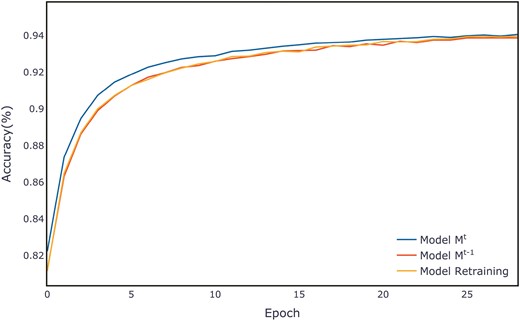
Using the ALOI dataset as an example, Fig. 6 displays the average accuracy per epoch on the validation set for three models on the ALOI dataset. Our proposed IAL-KD model begins with strong performance and rapidly converges to achieve a high level of accuracy. The training processes for all other datasets are illustrated in Figs A1–A11 in Appendix A. A detailed discussion of the performance across all datasets will be provided in the discussion section.

Average evaluation per epoch on the ALOI validation set.
Figure 7 shows the evaluation metrics on the test set for three models after multiple training sessions. Compared to the retrained model and the old model, the new model demonstrates a more concentrated distribution, maintaining a smaller range at higher evaluation metrics. The distribution of evaluation metric scores during the training process for each dataset can be found in Appendix B, in Figs B1–B11.
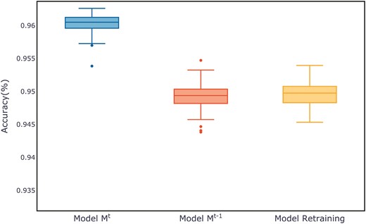
Comparison of evaluation metrics on the ALOI test set.
We also compared our method with the previously proposed incremental algorithm, ILIA. As shown in Table 4, the ILIA algorithm fails to meet task requirements on complex, large-scale datasets, showing a significant decline in performance and a decreased ability to process original data formats, resulting in a high FR according to equation (6). In contrast, our model achieved an average accuracy improvement from 69.32 to 75.39% in classification tasks, representing a 7.97% relative performance increase, all while reducing training time.
Comparison with existing IAL methods.
| Our IAL-KD | ILIA | |||||
|---|---|---|---|---|---|---|
| Time(s) | FR | Accuary | Time(s) | FR | Accuary | |
| Helena | 23.23 | 0.41% | 37.48%† | 203.60 | 11.74% | 33.09% |
| Jannis | 67.11 | 0.35% | 71.74%† | 465.97 | 7.10% | 66.47% |
| ALOI | 195.38 | -0.92% | 96.03%† | 325.81 | 8.61% | 86.17% |
| Covtype | 2429 | -0.68% | 96.30%† | 29940 | 2.87% | 93.54% |
| Average | 678.68 | -0.21% | 75.39%† | 7733.85 | 7.58% | 69.82% |
† is the best-performing model
To further investigate, we conducted multiple incremental experiments to assess whether the performance of older data formats deteriorates under the new model in a multi-increment scenario. As shown in Table 5, we performed a five-stage incremental experiment. Then, based on equation (7), we calculated the FRs for each stage. Without specifically learning the old format data, our model still maintained good classification performance and a low FR on the old data format, with each FR being around 1%. In many datasets, there was even a negative FR (the old format data performed even better on the new model).
FRs by data format across five stages.
| Dataset | Stage1 | Stage2 | Stage3 | Stage4 | Stage5 |
|---|---|---|---|---|---|
| Adult | 0.70% | 1.23% | 0.28% | 0.03% | 0.03% |
| Higgs Small | 1.77% | 6.56% | 0.76% | 0.28% | 2.11% |
| Helena | 0.41% | 5.66% | 5.87% | |$-$|0.14% | |$-$|0.06% |
| Jannis | 0.35% | 1.38% | 0.69% | 0.08% | 1.71% |
| ALOI | |$-$|0.92% | |$-$|1.27% | |$-$|0.71% | |$-$|0.95% | |$-$|0.86% |
| Covtype | |$-$|0.68% | 1.38% | 0.69% | 0.08% | 1.71% |
| Cal Housing | 4.83% | 2.40% | 10.31% | 8.02% | 1.13% |
| YEAR | |$-$|0.54% | 0.60% | |$-$|0.15% | |$-$|0.69% | 0.48% |
| Yahoo | 0.23% | 0.48% | 0.33% | 0.66% | 0.43% |
| Microsoft | 1.49% | |$-$|0.35% | |$-$|0.06% | 1.84% | |$-$|0.06% |
| Average | 0.764% | 1.807% | 1.801% | 0.921% | 0.662% |
5.2 Ablation study
To assess the individual contributions of the feature transformation module and the distillation module in the IAL model design, we conducted an ablation study. We replaced the feature transformation module with a standard fully connected layer to determine its impact on output consistency between the teacher and student models. Additionally, we investigated two approaches regarding regularization: one without using the distillation loss, and the other using the Fisher matrix for EWC regularization in an incremental method. We compared various aspects, including the number of parameters, training time, and evaluation metrics, to understand the role of each component in the model’s performance.
Table 6 presents the results of the ablation study conducted on our proposed model. Our model, which integrates both a feature transformation layer and a distillation method, achieved superior performance across most datasets, except for the Helena and California housing datasets. Modifying either the feature transformation layer or the distillation method resulted in a noticeable decline in overall model performance. Notably, the Helena and California housing datasets are the smallest and simplest among those tested, likely explaining the minimal performance differences observed between the various models. The model utilizing EWC regularization ranked just below our model in performance, indicating the benefits of regularization. However, despite the performance enhancement shown in the table, the EWC method increased the training time by ∼15% compared to the distillation method. These findings underscore the positive impact of both the feature transformation module and the distillation loss function on the model’s performance metrics.
Results of ablation study on proposed model.
| Feature | |$\checkmark$| | |$\times$| | |$\checkmark$| | |$\checkmark$| |
|---|---|---|---|---|
| Transformation | ||||
| Regularization | KD | KD | |$\times$| | EWC |
| Method | ||||
| Adult | 85.53% | 85.49% | 85.42% | 85.58%† |
| Higgs Small | 72.09%† | 72.07% | 71.58% | 71.85% |
| Helena | 37.48% | 37.73%† | 37.10% | 37.38% |
| Jannis | 71.74%† | 71.35% | 70.79% | 71.50% |
| ALOI | 96.03%† | 94.79% | 95.04% | 95.78% |
| Covtype | 96.30%† | 95.69% | 95.36% | 96.10% |
| CLS_AVG | 76.53%† | 76.19% | 75.88% | 76.36% |
| Cal Housing | 0.5512 | 0.5438 | 0.5374† | 0.5488 |
| YEAR | 8.8363† | 8.8660 | 8.8681 | 8.8484 |
| Yahoo | 0.7673† | 0.7675 | 0.7682 | 0.7677 |
| Microsoft | 0.7581† | 0.7584 | 0.7584 | 0.7582 |
| REG_AVG | 2.7282† | 2.7339 | 2.7330 | 2.7307 |
† is the best-performing model
When we revisit the training curve of ALOI without employing the feature transformation layer method in Fig. 8, it is observed that, in comparison to the original Fig. 6, the model has lost its capability for rapid convergence. This demonstrates the effectiveness of the feature transformation layer we proposed.
Model without feature transformation module: average evaluation per epoch on the ALOI validation set.
To further explore the impact of hyperparameter selection on our model’s performance, we conducted additional ablation experiments focusing on key hyperparameters: the temperature |$\tau$| and the learning rate decay factor |$\alpha$|, to find the best combination that maximizes the performance of the student model. Specifically, we selected temperatures |$\tau$| of 2, 3, 5 and different learning rate decay factors |$\alpha$| of 0.9, 0.95, and 0.98. The experimental results are shown in the Table 7 below:
Impact of temperature and learning rate decay on model performance.
| |$\boldsymbol{\tau }$| | |$\boldsymbol{\alpha }$| | Accuracy | FR |
|---|---|---|---|
| 1 | 0.9 | 37.23% | 1.39% |
| 1 | 0.95 | 36.73% | 0.40% |
| 1 | 0.98 | 36.16% | 0.32% |
| 3 | 0.9 | 37.50% | 1.66% |
| 3 | 0.95 | 37.48% | 0.41% |
| 3 | 0.98 | 37.02% | 0.43% |
| 5 | 0.9 | 37.81% | 2.38% |
| 5 | 0.95 | 36.64% | 1.27% |
| 5 | 0.98 | 37.22% | 0.86% |
The results indicate a clear trend regarding the influence of temperature (|$\tau$|) and the learning rate decay factor (|$\alpha$|) on model performance and FR. Lower values of |$\tau$| lead to a decline in performance, as seen with |$\tau = 1$|. When |$\tau$| is set to 3 or 5, the performance differences are minimal, but higher values are associated with an increase in the FR. For the learning rate decay factor |$\alpha$|, both excessively high and low values result in performance degradation, with lower values leading to higher FRs.
The optimal performance is achieved when |$\tau$| = 3 and |$\alpha$| = 0.95, resulting in favorable evaluation metrics and a low FR. Although the choice of hyperparameters does impact performance, the model generally outperforms the retraining baseline (accuracy 36.28%) across most hyperparameter settings.
6. Discussion
A paramount challenge in the realm of incremental learning is the integration of new knowledge without compromising the retention of previously acquired information. This study introduced a novel paradigm leveraging self-distillation and cross-modal distillation strategies to address this challenge. The redesign of the loss function and embedding layer algorithm specifically for incremental learning has proven effective in mitigating catastrophic forgetting. It has also enhanced the model’s adaptability to the unpredictability of input dimensions, thereby preserving the consistency of the model’s output across different stages of incremental learning.
Our proposed method employs both the old model and datasets in their original formats, subtly incorporating the nuanced transfer of knowledge enabled by KD (Hinton et al., 2015). This approach highlights the effectiveness of learning from an existing model to enhance a new one. Given the successful extraction of knowledge from the old model using KD, it is unsurprising that our model demonstrates commendable results. Unlike other forms of incremental learning, IAL faces the challenge of inconsistent input data formats. To address this, we introduced a feature transformation module. As detailed in Appendix A, except for the Adult dataset, our method’s ability to achieve high accuracy from the very first epoch is attributed to the successful “inheritance” of input from the existing model. Additionally, we observed that the model quickly reaches a peak performance higher than other models, and then starts to decline, indicating that the model trains faster and reaches the optimal point earlier. The Adult dataset did not demonstrate the characteristic of accelerated convergence in the first epoch, likely because the task is relatively simple, causing all models to converge within just one epoch.
Traditional methods often struggle with balancing new knowledge integration and old information retention. The integration of KD in our methodology allows for a more nuanced transfer and retention of information, ensuring model robustness and consistency across incremental updates. We addressed the issue of consistency at both the data and model levels, thus our model, compared to ILIA and retraining a model from scratch, demonstrates greater similarity with the old model in the final output layer (Table 8). This similarity between our model’s output and that of the original model indirectly evidences the continuity of our learning process.
Similarity with original model.
| Dataset | Our IAL-KD | Retraining | ILIA |
|---|---|---|---|
| Adult | 54.71% | 19.24% | ‒ |
| Higgs Small | 33.30% | 16.36% | ‒ |
| Cal Housing | 75.86% | 17.48% | ‒ |
| YEAR | 74.44% | 7.35% | ‒ |
| Yahoo | 65.37% | 3.05% | ‒ |
| Microsoft | 68.40% | 1.47% | ‒ |
| Average | 62.01% | 10.83% | ‒ |
| Helena | 65.22% | ‒ | 8.64% |
| Jannis | 59.92% | ‒ | 31.06% |
| ALOI | 69.19% | ‒ | 0.73% |
| Covtype | 59.65% | ‒ | 25.56% |
| Average | 63.50% | ‒ | 16.50% |
Another advantage of our proposed method is its low generalization error. As shown in Appendix B, our model, except for the Epilson and Helena dataset, has a significantly lower likelihood of producing poor evaluation metrics, indicating increased robustness and reliability. This effect is particularly pronounced in multi-class classification tasks. This phenomenon is akin to the self-distillation effect caused by softening hard targets (Pham et al., 2022). The lack of a significant advantage for the Epilson dataset may be attributed to the fact that it is the dataset with the highest number of features (2000 features), as shown in Table 2. Furthermore, these 2000 features have temporal relationships, which means that masking individual features does not significantly impact the model’s performance.
Compared to existing studies such as Lee (2023), which explore static environments for incremental learning, our study introduces a dynamic approach by continuously adapting the model to new data attributes. This represents a significant strength by offering a more flexible solution adaptable to real-world data evolution. However, a potential weakness lies in the increased computational complexity introduced by the KD process. Nonetheless, our tests indicate that the addition of the distillation loss function has a minimal impact on the backpropagation training time, with the average difference per epoch being <10%. Additionally, our method’s faster convergence reduces the required number of epochs, ultimately leading to a decrease in overall training time.
As shown in Table 4, our training time is significantly shorter compared to original IAL methods. As seen in Appendix A.1, our model reaches peak performance earlier and begins overfitting on the validation set. For scenarios requiring shorter training times, training with fewer epochs, as demonstrated in Table 3, can still yield relatively good results. Except for the complex Covtype dataset, rapid training with only five epochs performed well, even achieving the best performance on the datasets with relatively simpler tasks, such as Adult, Epsilon, and ALOI. This improvement is likely due to the reduced number of training epochs, which helps to avoid overfitting.
Regarding model size, the difference between the newly trained model and the previous model is confined to the mapping dimensions of the feature transformation module. This leads to minor variations in parameter size, which are insignificant when considering the overall model size. However, we must point out that to enable the model to effectively learn from the original model and data, additional storage space is required to retain the soft labels or feature vectors from the output layer of the original model. This storage space is closely related to the number of samples N and does not increase with the input feature dimensions. Specifically, the required space is calculated as |$N \times 339 \times 4$| bytes for regression or binary classification, or |$N \times$| the number of output classes |$\times 4$| bytes for multi-class classification. For example, for the Helena dataset, which is 7.7MB, ∼5.11MB of additional storage space is needed.
Despite our method’s superior performance across several datasets, we acknowledge some limitations. Our study primarily focused on tabular data, and the effectiveness and approach of KD on other data types such as images or text might require further exploration and validation. While our findings substantiate the potential of KD in incremental learning, they also underscore the necessity for further exploration into optimizing these models for practical, large-scale applications. Future research should aim to refine distillation and incremental learning processes to minimize computational demands without compromising model performance and to find methods to steadily improve model performance as new attributes are added. In future work, we will explore the possibility of refining and selecting soft labels or intermediate vectors to more effectively learn from the original model.
7. Conclusions
Current incremental learning techniques face significant challenges in adapting to new attributes without losing proficiency in previously learned information, especially when dealing with heterogeneously structured, variably dimensioned data. Our IAL-KD approach effectively tackles the issue of catastrophic forgetting by incorporating a KD method, ensuring that the model retains its ability to generalize from previously learned data while integrating new attributes. Additionally, our proposed embedding layer algorithm is specifically designed to handle the variability of input features, further enhancing the model’s adaptability.
We validated our method across 11 tabular datasets, encompassing binary classification, multi-class classification, and regression tasks. The experimental results demonstrated that our model outperforms traditional incremental learning methods and conventional retraining techniques, achieving a 7.97% improvement in classification tasks compared to existing methods (Gepperth & Hammer, 2016), while requiring significantly less training time. This efficiency is achieved without compromising the model’s performance on new data formats or forgetting old data. The FR on old data is ∼1% per incremental iteration. Furthermore, ablation experiments confirmed the effectiveness of our proposed modules.
This research extends existing distillation-based incremental learning methods into the realm of IAL, thus offering a promising pathway to enhance model adaptability and longevity.
In conclusion, our work demonstrates that KD can significantly enhance IAL systems, providing a viable solution to the challenges of adapting to new attributes while retaining previously learned information. This paves the way for the development of more adaptive and efficient machine learning models capable of handling dynamic data environments.
Conflict of interest statement
The authors declared no potential conflicts of interest with respect to the research, authorship, and/or publication of this article.
Author contributions
Zhejun Kuang (Conceptualization, Writing – review & editing, Data curation), Jingrui Wang (Writing – original draft, Software), Dawen Sun (Supervision, Funding acquisition), Jian Zhao (Resources, Validation), Lijuan Shi (Project administration), Xingbo Xiong (Investigation)
Acknowledgement
This work is supported by the Natural Science Foundation of Jilin Province (20210101477JC), the Education Department of Jilin Province (JJKH20230680KJ), and the Department of Science and Technology of Jilin Province (YDZJ202303CGZH010)
The author(s) declare that generative AI tools, GPT-4, have been used solely for translation assistance, copy editing, and grammar enhancement in this work. The author(s) have carefully reviewed and edited the content after utilizing these tools, and take full responsibility for the final content of the publication.
References
A Appendix
A.1 Experiments A
This appendix presents the complete experimental results of the average evaluation per epoch on the validation set. (Note that due to the varying number of epochs required for each training run, some sessions may have terminated early, resulting in fewer samples and greater fluctuations in the latter epochs.)
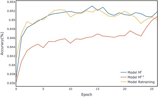
Average evaluation per epoch on the Adult validation set.
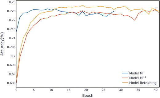
Average evaluation per epoch on the Higgs small validation set.
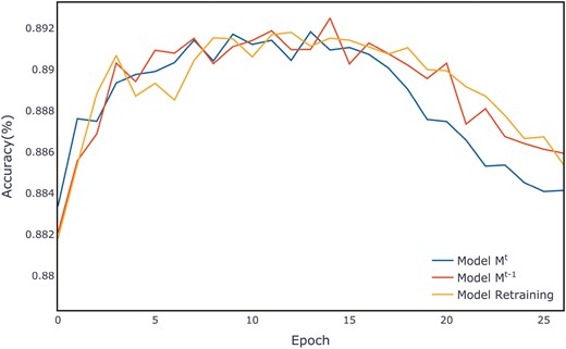
Average evaluation per epoch on the Epsilon validation set.
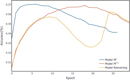
Average evaluation per epoch on the Helena validation set.

Average evaluation per epoch on the Jannis validation set.
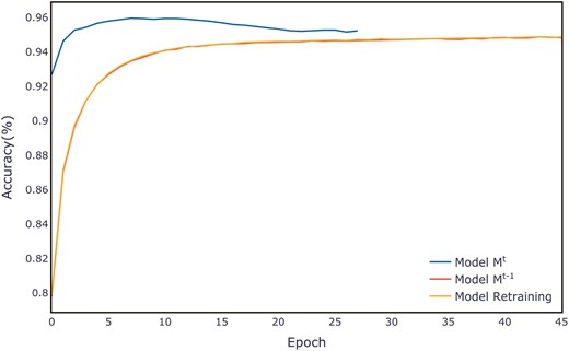
Average evaluation per epoch on the ALOI validation set.
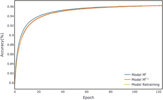
Average evaluation per epoch on the Covtype validation set.
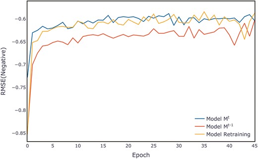
Average evaluation per epoch on the California housing validation set.
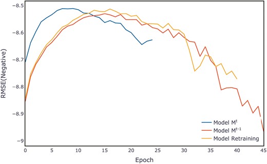
Average evaluation per epoch on the YEAR validation set.

Average evaluation per epoch on the Yahoo validation set.
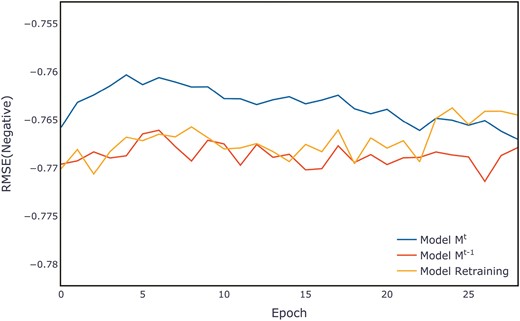
Average evaluation per epoch on the Microsoft validation set.
A.2 Experiments B
This appendix is the complete experimental result of the comparison of evaluation metrics on the test set
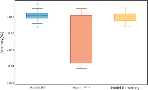
Comparison of evaluation metrics on the Adult test set.
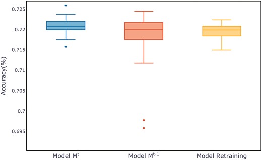
Comparison of evaluation metrics on the Higgs small test set.
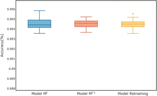
Comparison of evaluation metrics on the Epsilon test set.
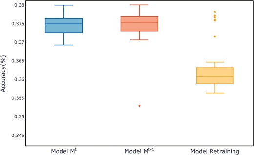
Comparison of evaluation metrics on the Helena test set.
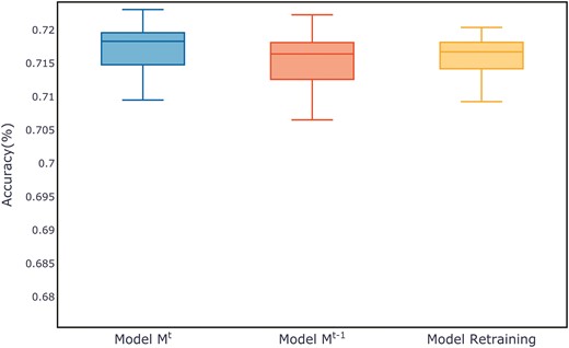
Comparison of evaluation metrics on the Jannis test set.

Comparison of evaluation metrics on the ALOI test set.
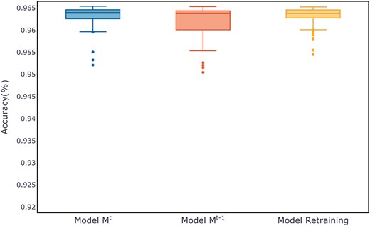
Comparison of evaluation metrics on the Covtype test set.
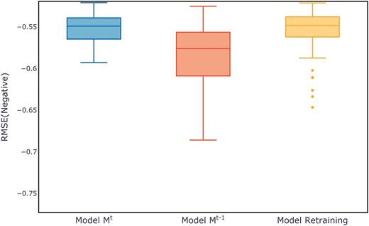
Comparison of evaluation metrics on the California housing test set.
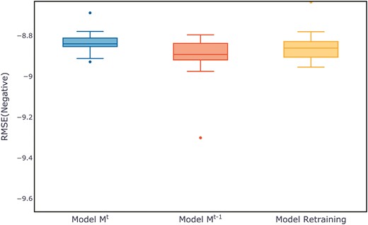
Comparison of evaluation metrics on the YEAR test set.
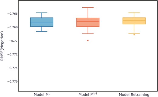
Comparison of evaluation metrics on the Yahoo test set.
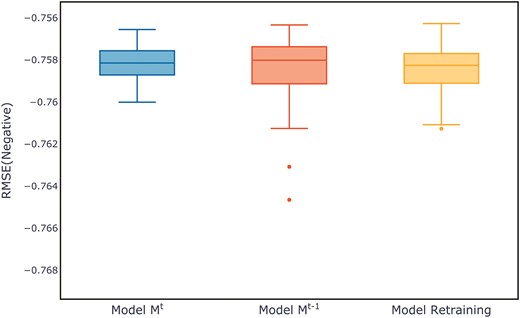
Comparison of evaluation metrics on the Microsoft test set.
