


Abstract
The goal of this research is to provide a novel conceptual base for ternary hybridity nanofluids that will improve heat transmission. This model illustrates how to produce heat conduction that is superior to the hybridity nanofluid. The ternary hybridity nanofluid is made by suspending three distinct kinds of nanostructures (TiO2, Al2O3, and SiO2) in ethylene glycol with varying physical and chemical linkages. The combination of these nanoparticles aids in the decomposition of hazardous compounds, environment cleansing, and the cooling of other equipment. This article describes the ternary hybrid nanofluids such as the conductivity of thermal and electrical, specific heat capacitance, viscosity, and density. The ordinary differential equations for the liquid and temperature are solved utilizing the Keller box method (KBM). The main finding discovered that the tri-hybrid nanofluid transferred more heat compared to the hybrid nanofluid. The velocity and temperature field diminishes for these ranges of parameters: |$0 \le \gamma \le 2$| (velocity slip|$\gamma $|) and |$0 \le {\gamma _1} \le 2\,\,$| (temperature slip |${\gamma _1}).\,\,$| The Darcy–Forchheimer |$Fr$| ranges between |$0.5 \le Fr \le 1.4$| diminishes the fluid velocity. The fluid moving subjected to a rotating cone has various applications in engineering like cone clutch, steam generators, loudspeaker cooling, lubricating grease for seals, hydrology, geosciences, etc.
Ternary hybridity Casson nanofluid non-Darcian flow and heat transfer with thermal radiation is evaluated.
Ternary hybridity nanofluid is made by suspending three distinct kinds of nanostructures (TiO2, Al2O3, and SiO2) in water.
Keller box method as numerical technique is used.
Tri-hybrid nanofluid is transferred more heat compared to the hybrid nanofluid.
Nomenclature
- |$Re$|
Reynolds number
- |${T_w}$|
Wall temperature (K)
- |${\lambda _1}$|
Porosity parameter
- |$Ec$|
Eckert number
- |$N{u_x}$|
Nusselt number
- |$Pr$|
Prandtl number
- |$Fr$|
Darcy–Forchheimer parameter
- |$\lambda $|
Buoyancy ratio parameter (N)
- |${\rho _{hnf}}$|
Hybrid nanofluid density |$\left( {\frac{{kg}}{{{m^3}}}} \right)$|
- |${C_p}$|
Specific heat at constant pressure |$\left( {\frac{j}{{kg - k}}} \right)$|
- |${\sigma ^{\rm{*}}}$|
Stefan-Boltzmann constant |$\left( {\frac{W}{{{m^2}{K^4}}}} \right)$|
- |${\gamma _1}$|
Temperature slip (K)
- |${T_\infty }$|
Ambient temperature (K)
- |$\beta $|
Fluid parameter (Pa.s)
- |$Gr$|
Grashof number
- |$C{f_x}$|
Skin friction
- |$Rd$|
Radiation parameter |$\left( {\frac{W}{{{m^3}}}} \right)$|
- |$qr$|
Radiative heat flux |$\left( {\frac{W}{{{m^2}}}} \right)$|
- |$\gamma $|
Velocity slip |$( {\frac{m}{s}} )$|
- |${\alpha _{hnf}}$|
Hybrid nanofluid thermal diffusivity |$\left( {\frac{{{m^2}}}{s}} \right)$|
- |${k_{hnf}}$|
Thermal conductivity |$\left( {\frac{W}{{m - k}}} \right)$|
- |${\kappa ^{\rm{*}}}$|
Absorption coefficient |$\left( {\frac{{{m^2}}}{{mol}}} \right)$|
Abbreviations
- PDEs
Partial differential equations
- KBM
Keller box method
- EG
Ethylene glycol
- HVAC
Heating ventilation air conditioning
- NPs
Nanoparticles
- EMHD
Electro magnetohydrodynamics
- MHD
Magneto hydrodynamics
- ODEs
Ordinary differential equations
- BVPs
Boundary value problems
- PC
Personal computer
1. Introduction
The process of transferring thermal energy from a higher temperature to a lower temperature in the same system is recognized as heat transfer. Temperature is the measurement of the hotness level of the system or object in the same region, where a higher temperature indicates that this system or object is hotter than the ambient system or another closer object. Moreover, temperature also indicates the thermal energy level of the system or object, where thermal energy is related to internal energy. The methods of transferring thermal energy are conduction, convection, or radiation. Conduction occurs in the conducting medium, where heat is transferred between in-contact neighboring molecules. Convection occurs when a density gradient exists in fluids, such as liquids and gases. Besides, radiation is contradictory compared to conduction: It is a process in which heat is propagated through electromagnetic waves, and the involved systems or objects do not need to contact each other. The applications which employed heat transfer are electronic device cooling (Gururatana, 2012), steam-electric power generation (Raptis et al., 2020), heating, ventilation, and air conditioning (HVAC) systems (Colangelo et al., 2021), biomedical simulation (Šterk & Trobec, 2005), etc.
Hybrid nanoparticles are made from the slightest exact nanometer sizes. This nanoparticle is then submerged into the liquid to form a nanofluid. However, using more than one nanoparticle will increase the fluid's thermal properties, and it is known as a hybrid nanofluid (Mehryan et al., 2019). Crossbreednanoliquids are prepared by dissolving particular assortments of NPs in basic liquids and springing up as unused nanotechnology (Sidik et al., 2017). Choi et al made use of nanofluid which labored at the tempo of depth circulation differentiated with unadulterated liquid (Choi & Eastman, 1995). Around that point, nanofluid got to be considered since it gave energizing outcomes to extend warmness circulate execution differentiated with refined liquid (Waini et al., 2020). This examination unfolded a distinctive method for designing frameworks due to the special effects within the wake of using nanofluids. A few exams had been completed and varieties of nanoparticles had been suspended in essential liquids. Nanofluid grows the beat of profundity circulate differentiated with nanofluid and smooth fluid. Peeri et al. (2020) attempted a mix of Multiwall/round silica nanotubes to breed nanostructures and warm execution ask approximately of the surveying nanofluid. Crossover nanoparticles are characterized as nanoparticles made from the slightest exact nanometer sizes. The fluid organized via way of means of the combination nanoparticles is referred to as go-breed nanofluids to lower any mono nanofluid deserts (Eid, 2022). Mixture nanofluids are extraordinarily a hit as a way of cooling while temperatures are excessive and contain several heat frameworks. Blended nanofluids are generally equipped via way of means of dissolving specific varieties of NPs in fundamental liquid and springing up as modern nanotechnology (Xian et al., 2018). Half-breed nanofluid appreciates a few points of interest differentiated from customary collections due to its balanced homes. Theire over-the-top arranged thermophysical and rheological homes cause them to be best for sun-based, completely based quality systems. In this review paper, an overview of sun-powered fueled quality systems is tended to, and from there on, the utilization of hybrid nanofluids in distinctive solar-orientated innovations, mainly daylight primarily based heat, is explored (Akilu et al., 2018). Relationships between nanofluidic systems and ordinary ones have been made to construct an additional significant comprehension of the endowments of utilizing nanofluids. As demonstrated via the assessed examination, the development of the effectiveness of nanofluidic planetary agencies may be credited to the developing heat residences of convective fluids. Furthermore, it tends to be assumed that nanofluids’ component essentially impacts how the systems work reasonably (Manjunatha et al., 2022). Khan et al. (2021b) pondered the dissipation effect and MHD on electrically conducting hybrid fluid moving across a needle. Rana & Gupta (2023) investigated the impact of non-linear mixed convection and Stefan blowing using the response surface method on fluid past a vertical cone. The impact of EHMD and nanoparticles on binary fluid moving subjected to a stratified medium is studied by Dawar et al. (2021). Rana and Gupta (2022a) investigated the impact of hybrid nanoparticles and Hall current effect on fluid flow subjected to a vertical cone and achieved the solution of the proposed model with the utilization of the finite element technique. Bilal et al. (2021) contemplated the performance of hybrid nanoparticles on fluid over a wavy spinning disk. Rana & Khurana (2023a) investigated the stability of a non-Newtonian nanofluid (Al2O3-EG) layer subjected to a chemical reaction, rotation, and magneto-convection. Khan et al. (2022c) investigated the impact of titanium alloy nanoparticles on magnetohydrodynamic flow through the Darcy–Forchheimer medium. Similar work on hybrid nanoparticles is mentioned in Rasool et al. (2022, 2023a, b, c; Li et al., 2023) for readers’ interest.
Tri-hybrid nanoparticles had been focused on with the aid of distinctive researchers. For instance, breed nanofluid appears extra extraordinary warm trade and rheological homes separated with crucial fluids and mono nanofluids (Nazir et al., 2021) study up crucial heat improvement for ternary hybrid nanoparticles while contrasted with the nice and cozy improvement for crossover nanofluid and nanoparticles in complicated liquid over a warmed two-layered outline. They performed in a restrained thing manner to cope with accomplishing mathematical outcomes. Chen et al. (2017) investigated hybrid nanoparticles with graphene oxide/graphene and MoS2/zirconia to describe the tribological and mechanical homes. Zayan et al. (2021) attempted a new triple combination nanostructure thinking about the nice and cozy introduced substances. Shafiq et al. (2021b) focused on Walters’ B fluid in nanoparticles thinking about double definition consisting of stagnation calculation employing a Riga plate. Significant another examination (Swain et al., 2021) tested highlights linked with crossover nanoparticles in the sight of a compound reaction in the direction of an extending floor consisting of slippage constraints. Research (Mebarek-Oudina et al., 2021) did a cherished adaptation outline concerning combination nanoparticles, engaging boundary thinking convection warmth control in a trapezoidal pit. Warke et al. (2022) scientifically inquired about the stagnating figure comportment within the location of warm radiative fluxing via a warmed floor. Dadheech et al. (2020) stuck the results connected with warmth control circulate within the location of crossbreed nanoparticles utilizing the method of passing breed nanoparticles below an appealing boundary. Marzougui et al. (2022) focused on entropy age and depth circulation incorporating nanoparticles in a cowl-pushed hollow space below an appealing subject. Mebarek-Oudina (2019) reproduced convective depth circulation employing a category of nanoparticles of titanium nanofluids utilizing warmth supply terms.
Subsequently, the following studies regarding the ternary combination nanostructures also reported: solar-powered gatherers (Dhif et al., 2021), mixed convection in an upward warmed channel with the aid of titanium nanofluids (Zamzari et al., 2015), the circulation and delineations in non-Newtonian fluid, tallying nanoparticles utilizing a non-Fourier strategy (Li et al., 2021a), Ferro-liquid convection in a warmed channel (Mehrez & Cafsi, 2021), the impacts of warm radiation on the nanofluid along the shape component (Khashi'ie et al., 2021), the impact of various consistency and hybrid nanoparticles on non-Newtonian fluid (Esfe et al., 2021), and hybrid nanofluid flow in a warmed pit through a throbbing channel condition (Mehrez & Cafsi, 2017). Ramesh et al. (2022a) investigated the influence of heat source/sink on ternary nanofluid moving across a slippery surface. The impact of heat source/sink on ternary hybrid nanofluid flow through converging/diverging channel were deeply investigated by Ramesh et al. (2022b). Rana and Gupta (2022b) studied Von Kármán's rotatory dynamics of nanoliquid over a disc with thermal and solute buoyancy forces. For readers’ interest, kindly check these references: Rana et al. (2022), Eswaramoorthi et al. (2023), Kumar et al. (2023), Shakeel et al. (2023), Yaseen et al. (2023), Zeeshan et al. (2023), and Zhang et al. (2023).
It is first-rate that a particular magnificence of contraption, just like a windmill, constantly ready, will pivot whilst the breeze blows, and the more prominent critical the breeze pace, the quicker the insurgency cost could. A vigorous cone turning in a liquid like water ought to involve the draw to disentangle nearby the center of the flip, base to begin with, and best final. What’s more noteworthy, the quicker the flip the more prominent and distinguished the weight is to decipher. What needs to emerge accepting that those partitioned intellects had endeavored to be coupled together? A handful of picks are provided underneath. To begin with, the turning/decoding cone thought did not come from taking note of nature, which has in some instances taken place inside the beyond via the fantastic gadget of improvement. A horn shark egg case induces several unsatisfactory ways for a brief period. It is ordinarily cone molded but after a long term inside the water, the unmistakable turning vane will end up vertical to the cone’s floor and set. Certainly, such an unordinary shape likely happened on purpose. The spiral ridges on the egg casing help it grasp rocky crevices where the mother normally deposits it. “It wedges into a rock really well, so if there’s surge and waves, it won’t move the egg, and it makes it harder for predators,”. Notwithstanding, the aid of using pushing numerous eggs with the assistance of using hand via the water in an aquarium tank, the anticipated response did not emerge. The turn ended unexpectedly after more than one insurgency. Essential to the modern concept may be a simple floor on the cone's side. A transformation of speculation disbursed in a recognizable liquid factors text (Batchelor, 1967) created the outcome. At the factor, whilst a robust chamber pivots at a constant price in a nevertheless liquid, there may be no touch inside the liquid and non-skilled with the aid of using the chamber. That a lot is remarkable without assistance from all and sundry else. In the previous article (Kenyon, 2020) the supposition that became made that there might likewise be no grinding assuming a robust cone pivoted in a liquid. Yet, that expectation need not hassle with to be made, in mild of the truth that it tends to be shown with the aid of using Navier–Stokes conditions in spherical and hole polar instructions (instead of aircraft polar instructions for the pivoting chamber), for the reason that type of the rotational pace element is instantly alongside the cone’s floor ordinary to the circulation bearing (Kundu, 1977). The different pace components observe the chamber’s model. The implementation of the stress pressure at the turning cone’s floor using Bernoulli’s law has been applied to the steady circulation in a close spherical smoothed out encompassing the cone. As a result, this likewise is not a presumption but speculation that as of now has visible more than one utilization (Kenyon, 2019). Also, self-reliant speculation withinside the liquid factors text (Kenyon, 2017) offers comparable effects for the pivoting chamber, for example, the tumble-off tempo of the afflicted pace far from the vigorous body (see condition 1), which other than does not make utilize of Bernoulli’s law, so 2 isolated hypotheses agree with one another. As demonstrated with the help of utilizing Bernoulli’s law the uneasiness is the slightest in which the rate is most critical. Appropriately the uneasiness at the cone’s floor closes the foot is diminished than on the summit. That is the approach with the help of utilizing the concept of elucidation happens.
The movement model of viscoelastic fluids, namely Casson fluid was developed by Casson in 1959. This is a plastic fluid model that shows the properties of shear thinning and viscosity, together with the yield stress. Blood is a perfect example of Casson fluid. A handful of exercises of Casson liquid are nectar, stick, sauce, etc. (Bhatti et al., 2016). The Casson liquid moves on an inclined sheet with the help of utilizing combining the Soret–Dufour impacts as reported by Ali et al. (2018). Khaled et al. (2015) centered on the Casson liquid movement on vertically skewed sheets. The influence of planned response on Casson fluid moves on a slanted plate is investigated by Shamshuddin et al. (2018). The inclination plate which acts as a boundary for the Casson fluid flow is analysed by Vijayaragavan & Kavitha (2018) utilizing the heat source/sink effect. Prasad et al. (2018) looked into the Casson liquid move over a skewed sheet with the assistance of utilizing considering around the entryway current. The skewed Casson liquid moves on a permeable sheet are studied by Jain & Parmar (2018). Sailaja et al. (2018) centered on the Casson liquid move on a vertical sheet with the assistance of utilizing joining the calculated effect. The Casson liquid bounded by a slanted sheet with the help of utilizing considering almost nanoparticles is explored by Ravi et al. (2017). Raju et al. (2017) evaluated the Casson liquid move-on in a vertical bearing inclined sheet. The Casson liquid version is greater affordable with circulatory device propagation. The effect of variable fluid houses in the move discipline is dissected with the aid of using thinking about a convective breaking factor condition. Power, power, and obsession situations are modified into the non-immediately trendy differential shape via right closeness adjustments and are treated efficaciously via the optimal homotopic analysis method (Rashidi et al., 2018). The effect of great limits on dimensionless pace, temperature, and middle are depicted graphically. The Casson fluid version carries zero nanoparticle mass extrude on the breaking factor nearby components of Brownian improvement and thermophoresis to chip away at the improvement of nanoparticles (Abbas et al., 2016). The idea of motile microorganisms is visible as useful for the unfaltering exceptional of the nanoparticles. We noticed that the move fields were painted on because of the development of variable heat conductivity but avoid enlargement in issue thickness and Casson fluid restriction. A boom in issue fluid thickness and Casson liquid restriction overhauls hotness and motile microorganism flow rates but reduces the mass conversion scale. The exposed discernments tune down programs in enrobing approaches for electric-conductive nanomaterials; may be utilized in flight, outstanding protecting delivery situations, polymer looking after, and numerous ventures. Saeed et al. (2022) investigated MHD Casson fluid flows over an expandable surface, and the flow is embedded with a chemical reaction. Thammanna et al. (2017) investigated the influence of MHD and chemical reaction on couple stress Casson fluid moving subjected to an unsteady surface. Ramesh et al. (2016) contemplated Casson fluid moving subjected to an elastic medium accompanied by thermal radiation and stagnation point. Sharma et al. (2023) investigated the impact of nanoparticles on Casson nanofluid with the consideration of water (Newtonian) and Blood as a non-Newtonian base fluid.
The slippery constraint connected to this show has the motion picture shearing strain on the divider relative to the rapidity of the motion picture on the divider (the Navier slippage circumstance) that is routinely carried out to scaled-down or nano-scale liquids. For bounder streams, the no-slip circumstance has been tended to as of late. On the challenge of holding halls, Kay (2013) confirmed movie tiers of a hundred μm, wherein floor effects of the chamber divider would possibly affect the growing movie. We do not know approximately the slip situation being applied for considerable scope liquid rimming streams, but a relative liquid circulation may be located in crafted with the aid of using study or examination of air greased up direction (Barber et al., 2004). The floor-to-quantity percentage activates floor effects overwhelming the movie elements. Khan et al. (2022b) investigated the impact of magnetic field and convective heat transfer on rotating viscoelastic fluid and observed that the velocity field diminishes under magnification in magnetic number. The effect of entropy generation and natural convection on fluid flow under the effect of Caputo hybrid and Atangana Baleanu fractional derivative were investigated in detail by Khan et al. (2021a).
An air greased-up push conserving on for the Navier slip situation is brought with the aid of using Bailey et al. (2015) wherein the important thing obstacles are tantamount to the tiny liquid thickness and the intermolecular remove. Constrained circumstances for circulation in a significantly sheared bearing chamber usually include the commonly stated no-slip restriction situation, applied from as quickly as 1738 with the aid of using Bernoulli for the liquid robust connection factor (Lauga et al., 2006). An incomplete slip restriction situation became an early notion with the aid of using Navier as indicated with the aid of using Neto et al. (2005) wherein a fluid would possibly slip throughout a robust floor whilst experiencing a contradicting pressure comparative with the robust velocity occurring from contact. This midway slip is for the maximum element characterized with the aid of using a slip period, extensively stated in comparing the slip of fluid on the robust floor. Additionally, there may be limited circumstances of stale layer and total slip for perfection (Eijkel, 2007). The slip circumstance is exceptionally connected to floor treatment alternatives at the strong floor for a fragmentary slip imprisonment circumstance, which is investigated by Choi et al. (2003). It is observed that a hydrophobic floor brought longer slippery lengths than a hydrophilic floor for water, up to three |$\mu \mathrm{ m}$|. Progress examinations on hydrophilic and hydrophobic plates had been made by Cottin-Bizonne et al. (2002), in the conditions that hydrophilic surfaces utilize the no-slippery circumstance and hydrophobic plates had higher slip lengths than a few μm. In this study, speculating nano-air wallets would conceivably hydrophobic plates had higher slippery lengths than a few μm. Khan et al. (2022a) scrutinized the effect of velocity slip and entropy generation on magnetized Casson fluid. A charming recommendation for the slippery limitation circumstance is in the water-fueled breaking of shale, wherein Javadpour et al. (2015) studied the slippery lengths in scaled-down nano streams for homegrown pores of a shale system. The significance of slip in shale nanopores and water-fueled splitting is also being reported. Referring to Hu and Granick’s study, liquid slip influences shear costs, and floor influences act as tribology strategies for nanometer motion picture thicknesses (Hu & Granick, 1998). The Navier slippage adaptation is characterized as a consistent slippage version, with an immediate connection among the extraneous shear price and the factor of interplay velocity contrasts, wherein the slip period is going approximately because of the regular proportionality. The true situation nonetheless cannot appear to be shown for all programs due to the intricacy related to character effects, for example, floor harshness of the relationship factor or the wettability of the floor. Uddin et al. (2023) investigated the effect of second-order slip and bioconvection on micropolar fluid flow subjected to a vertical cone through porous media. Shah et al. (2023) scrutinized the effect of MHD and free convection on viscous fluid flow through parallel vertical plates. Souayeh et al. (2019) probed the influence of Titanium alloy and ferromagnetic nanoparticles on dusty liquid flowing subjected to a slippery surface embedded with thermal radiation effect.
The flow rate and pressure are linearly related to each other and applicable in the case of |$Re < 1$| and low-velocity situations. Forchheimer resolved this issue by taking the quadratic power of a velocity term later called the Darcy–Forchheimer flow term. The Darcy–Forchheimer phenomenon is utilized where the velocity of the fluid is high enough and |$Re > 1$|. Alharbi et al. (2022) studied the model of a Darcy ternary hybrid nanofluid over an expandable cylinder. Micropolar fluid subjected to a porous stretchable sheet and thermal radiation is scrutinized by Bilal et al. (2022). Díaz Palencia (2022) solved the mathematical model of MHD Darcy–Forchheimer fluid flow. Ullah et al. (2022) evaluated the entropy generation of a hybrid nanofluid through a Darcy–Forchheimer medium. Muhammad et al. (2022) studied the hybrid nanofluid flow passing through a Darcy porous medium. Darcy–Forchheimer fluid flow subjected to a stretching rotating inclined disk was reported by Adnan et al. (2022). MHD hybrid nanofluid flow through the Forchheimer medium with the implementation of thermal conductivity was reported by Shafiq et al. (2021a). Rasool et al. (2021) implemented the Darcy–Forchheimer relation on magnetically driven Jeffrey fluid subjected to an elastic surface. The Casson–Carreau nanofluid model embedded with an active energy phenomenon is developed by Ali et al. (2020).
1.1 Motivation
The hybrid nanofluid flows over a rotating cone with the inclusion of various effects has been investigated by many researchers as shown in the literature review section. There is still a gap available in the literature on a fluid bounded by a rotating cone with the consideration of various effects. The article fills the gap with the consideration of trihybrid nanomolecules on the fluid moving subjected to a slippery rotating cone never investigated before. This study describes how fluid behaves by adding tri-hybrid nanoparticles subjected to a slippage plate with the insertion of the Darcy effect has been deeply investigated in this study.
1.2 Novelty
The novelty behind the present research is given below.
The effect of ternary hybrid nanoparticles on the fluid moving over a rotating cone is not investigated yet in the available literature.
Darcy–Forchheimer and porosity effects have not been taken simultaneously in order to study the fluid flow behavior over the rotating cone.
In the instance of liquid flowing via a cone, the Maxwell rapidity slip and Smoluchowski temperature slippage boundary constraints have not been considered in the previous study.
2. Mathematical Formulation
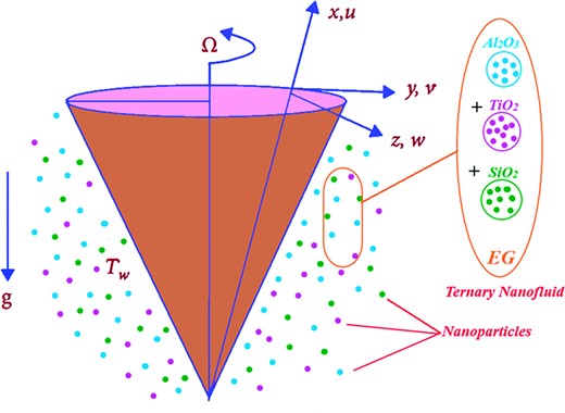
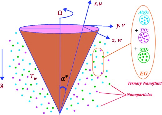
Figure 1 shows the modelling of a mixed convective Casson fluid embedded with ternary hybrid nanoparticles using ethylene glycol as the base fluid past a porous vertical cone. Darcy–Forchheimer is considered to study fluid behavior. The cone is moving subjected to an angle |$\Omega$| and the buoyancy-driven effect is mentioned by |$\text {g}$|. Because of the buoyancy-driven mixed convection effect used in the momentum equation, Boussinesq’s approximation is used, and free convection flow is considered in the present model. Rosseland radiative heat flow is considered, and the medium is optically thick and porous. At the exact location of the sheet, the Maxwell rapidity slippage and Smoluchowski temperature slippage are regarded as boundary constraints. The parameters |${U}_w$| and |${U}_\infty $| depicts the stretching velocity and ambient velocity. The temperature at the wall and ambient temperature are represented by |${T}_w$|,|${T}_\infty $|. Further, it is assumed that |${T}_w > {T}_\infty $|. The gravitational acceleration is directed normally to the cone position and the cone half angle is |$\alpha^* $|. The related profiles (velocity and temperature) are different at any location, for example: at the sheet or any point in the fluid. Meanwhile, Darcy’s law is valid where the velocity of the fluid is low and |$Re < 1$|. In the case of Darcy’s law viscous forces dominate inertial forces. Forchheimer extended the Darcy law by taking the square term and applicable where fluid flow and pressure are in a non-linear relationship. Darcy–Forchheimer term where the velocity of the fluid is high and |$Re > 1$|, and it is included in the momentum equation. The pertinent effects like density, specific heat, and thermal conductivity of ternary hybrid nanofluid are manifested by the symbols |$\ {\rho }_{Thnf}$|, |${(\rho {C}_p)}_{Thnf}$|, and |${k}_{Thnf}$|.
Flow diagram.
Limitations of the present model
Mixed convective Casson fluid is considered.
Cone is rotating with a rotating angle |${\rm{\Omega }}.$|
Agglomerative nanoparticles like ternary, di-hybrid, and mono are considered for heat transfer analysis.
Maxwell velocity and Smoluchowski slip conditions are considered at the surface of the cone.
The continuity equation is automatically satisfied. The governing modeled equations in terms of continuity, momentum, and temperature equations (Li et al., 2021b; Mogharrebi et al., 2021) together with the related boundary conditions are mentioned underneath:
where |$F = \frac{{{C}_b}}{{\sqrt {{K}^*} }}$|. The thermophysical properties of ternary hybrid nanofluid are (Ramesh et al., 2016; Thammanna et al., 2017)
Thermophysical properties of Al2O3, TiO2, and SiO2 nanoparticles and EG basefluid are presented in Table 1.
Thermophysical properties.
| Properties | Ethylene Glycol (EG) | Al2O3 | TiO2 | SiO2 |
|---|---|---|---|---|
| |$\rho $| | 1115 | 6310 | 4250 | 2270 |
| |${C_p}$| | 4179 | 773 | 690 | 765 |
| k | 0.253 | 32.9 | 8.953 | 1.4013 |
| Properties | Ethylene Glycol (EG) | Al2O3 | TiO2 | SiO2 |
|---|---|---|---|---|
| |$\rho $| | 1115 | 6310 | 4250 | 2270 |
| |${C_p}$| | 4179 | 773 | 690 | 765 |
| k | 0.253 | 32.9 | 8.953 | 1.4013 |
The expression regarding Rosseland approximation is
whereas |${\sigma }^{\rm{*}}$| and |${\kappa }^{\rm{*}}$| relatively depicts Boltzmann constant and absorption coefficient, respectively.
3. Solution Methodology
The appropriate conversions are presented below (Raju et al., 2017; Ravi et al., 2017; Sailaja et al., 2018)
The above conversion will transform (2–6) as below (Neto et al., 2005; Eijkel, 2007):
In (9–12), the occurring dimensionless parameters are expressed as
The local Skin friction coefficient and Nusselt number are given by (Neto et al., 2005; Eijkel, 2007)
whereas the shear stresses |${\tau }_{xz}$|, |${\tau }_{yz}$|, wall heat flux |${q}_w$| are premeditated by
The dimensionless form of surface drag is expressed in (15–16), whereas the Nusselt number is in (17; Cottin-Bizonne et al., 2002; Choi et al., 2003; Neto et al., 2005; Eijkel, 2007; Javadpour et al., 2015; Kenyon, 2017; Khan et al., 2022c),
whereas |${A}_1$|, |${A}_2$|, |${A}_3$| are given by (Ramesh et al., 2016; Thammanna et al., 2017),
The comparison of skin friction coefficient values with Chamkha & Al-Mudhaf (2005) and Malik et al. (2016) for diverse values of buoyancy parameter |$\lambda $| is tabulated in Table 2. Table 3 displayed the comparison analysis of the obtained results with Saleem and Nadeem (2015) in the case of heat transfer Nusselt number by keeping |$Pr$| fixed and varying |$\lambda $|. From comparison analysis, as shown in Tables 2 and 3 the obtained results are quite satisfactory and the proposed numerical scheme is quite reliable.
Comparison in the case of Nusselt number with Saleem and Nadeem (2015).
| Parameters | Saleem and Nadeem (2015) | Present | |
|---|---|---|---|
| |$Pr$| | |$\lambda $| | |$N{u_x}$| | |$N{u_x}$| |
| 0.7 | 0.0 | 0.4299 | 0.4280 |
| 0.7 | 1.0 | 0.6121 | 0.6519 |
| 0.7 | 10 | 1.3992 | 0.3989 |
| Parameters | Saleem and Nadeem (2015) | Present | |
|---|---|---|---|
| |$Pr$| | |$\lambda $| | |$N{u_x}$| | |$N{u_x}$| |
| 0.7 | 0.0 | 0.4299 | 0.4280 |
| 0.7 | 1.0 | 0.6121 | 0.6519 |
| 0.7 | 10 | 1.3992 | 0.3989 |
4. KBM: Second Order Convergent
When outcomes obtained from any method are closer to real-life situations as well as approximately near to exact solutions obtained with some limitations, that method is considered as most efficient.
There are four steps involved in the KBM to obtain the solution of an equation. These factors are mentioned below:
Transform the system of equations into a first-order system.
Convert the first-order system of equations into difference equations utilizing central differences.
Linearize the system of equations and arrange them in matrix-vector form.
At the end solve that linear system of equations with the block-tridiagonal elimination method.
The Keller box method (KBM; Keller, 1971) is one of the favoured analytical schemes utilized in solutions of BVPs. This approach is still one of the most powerful, adaptable, and accurate finite-difference methods used in current viscous fluid dynamics simulations. This numerical scheme is unconditionally stable and provides a second-order convergence criterion. Crucial criteria of KBM were tackled by the Von Neumann process, which gives a certificate for the present numerical study with stabilization of procedure. Numerous published findings have verified the approach, which provides great mesh sensitivity testing to select the optimal grid spacing for computing quickly converging solutions for boundary layers. It also improves viscidity and convergence of numerical solution obtained for Equations (2–5) through the KBM. Grid independence tests were used in this work to validate the correctness of the Keller-box code. Stepwise progress in KBM is described in a flow chart (Fig. 2).
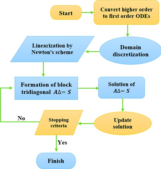
Flow chart illustrating the KBM.
KBM has executed to verdict the solution of exhibited formulas resulting from the rapid convergent. The limited solution of the formulas (9–11), with constraints (12), is created utilizing KBM. The procedure of KBM is identified as follows:
The initial step is alteration all ODEs (9–12) into ODEs of the first order, i.e.,
4.1 Conversion of ODEs
We start by introducing new independent variables:
|$Z{G}_1( {x,\eta } )$|, |$Z{G}_2( {x,\eta } )$|, |$Z{G}_3( {x,\eta } )$|, |$Z{G}_4( {x,\eta } )$|, |$Z{G}_5( {x,\eta } )$|, |$Z{G}_6( {x,\eta } )$|, and |$Z{G}_7( {x,\eta } )$| with |$Z{G}_1 = f$|, |$Z{G}_2 = f^{\prime}$|, |$Z{G}_3 = f^{\prime\prime}$|, |$Z{G}_4 = g$|, |$Z{G}_5 = g^{\prime}$|, |$Z{G}_6 = \theta $|, and |$Z{G}_7 = \theta ^{\prime}$|. Because of this transformation, Equations (9–11) reduce to the following first-order form
4.2 Domain discretization & difference equations
Furthermore, domain discretization in |$x - \eta $| plane is represented in Fig. 3. Because of this mesh, net points are |${\eta }_0 = 0,{\eta }_j = {\eta }_{j - 1} + \delta L,\ \ \ j = 0,1,2,3...,J,{\eta }_J = 1$| where |$\delta L$| is the stepsize.
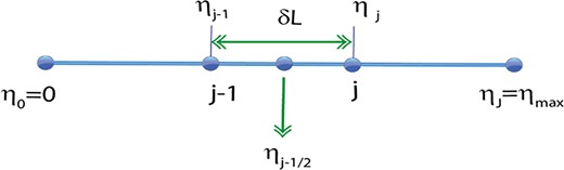
A Keller-box computational cell and grid meshing.
Applying central difference formulation at the midpoint |${\eta }_{j - 1/2}$|
4.3 Newton method
Equations (27–33) are linearized employing Newton’s linearization method
Substitute the expressions obtained in (27–33) and dropping the square and higher powers of |$\delta $|, the following set of equations is achieved:
where
4.4 Block tridiagonal structure
In the end, the above formulas are employed and a bulk tri-diagonal array is obtained as:
where
where the elements defined in Equation (45) are
Now we factorize A as
where
Here A is representing a block matrix having a |$5 \times 5$| size corresponding to a generalized matrix having |$J \times J$| size. While |${\rm{\Delta }}$| and S are representing column-vectors having |$J \times 1$| order. An efficient LU factorization method is employed to obtain the solution of |${\rm{\Delta }}$|. Equation |$R{\rm{\Delta }} = pA{\rm{\Delta }} = S$| is demonstrating the fact that matrix A is acting along with |${\rm{\Delta }}$| to produce S as vector output. After that, R is splinted in lower and upper trigonal matrices, i.e., |$A = LU$| can also be written as |$LU{\rm{\Delta }} = S$|. Consider |$U{\rm{\Delta }} = y$| tends to |$Ly = S$| which helps provide the solution for y. Then calculated y values are added in |$U{\rm{\Delta }} = y$| to obtain solutions of |${\rm{\Delta }}$|. Back-substitution method is employed as it is very easy for obtaining a solution for triangular matrices. The number of mesh points influences the numerical output. After a few trials, a higher number of mesh points are chosen in the η-direction. The maximum value has been set to |${\eta }_{max} = 9$|, which defines an appropriately big number at which the necessary boundary requirements are met. For this flow domain, the max value is set to |${\eta }_{max} = 9$|. Mesh independence is therefore attained in the current computations. The algorithm’s computer software is run on a PC using MATLAB. According to Keller, the approach has great stability, convergence, and consistency. As demonstrated in Table 4, the solution is totally grid independent for all approved selections of the parameters specified in the paper.
Grid independence test for the existing model’s convergent solution for sufficient levels of involved flow restrictions.
| Step size | Grid points | |$- f^{\prime\prime}( 0 )$| | |$- g^{\prime\prime}( 0 )$| | |$- \theta ^{\prime}( 0 )$| |
|---|---|---|---|---|
| 0.1 | 90 | 2.603494 | 1.720234 | 2.002587 |
| 0.02 | 450 | 2.603491 | 1.720146 | 2.002694 |
| 0.01 | 900 | 2.60349 | 1.720143 | 2.002697 |
| 0.006 | 1500 | 2.60349 | 1.720143 | 2.002698 |
| 0.005 | 1800 | 2.60349 | 1.720143 | 2.002698 |
5. Results and Discussions
Symbol ‘|$\beta $|’ depicts the viscosity index of the Casson fluid parameter. Fluid is a shear thickening in the case of |$\beta > 1$|, shear thinning in the case of |$\beta < 1,$| and Newtonian for |$\beta = 1$|. A Casson fluid is the most suitable rheological model for blood and other non-Newtonian fluids. Casson fluids hold yield stress and have great significance in biomechanics and polymer industries. Forchheimer number (|$Fr$|) is used in the case where the change in pressure is directly proportional to the square of the velocity term for the case of fluid flow, as is the case with Forchheimer number (|$Fr$|), and when the high velocity of the fluid flow is necessary, Forchheimer number (|$Fr$|) is used. The porosity of the medium is represented by the dimensionless symbol |${\lambda }_1$|. The capacity of a medium to transport fluid is referred to as the medium’s permeability. Porosity is related to permeability. While a low porosity almost always leads to a low permeability, having a high porosity does not always mean that it will have a high permeability. When the fluid is allowed to flow through a more porous material, the physical environment is improved. The ratio of buoyancy to thermal diffusivity is referred to as the Rayleigh number |$\ \lambda $|. The amount of heat transfer that may be attributed to natural convection processes can be measured with the use of a statistic called the Rayleigh number. If the Rayleigh number is smaller than the critical value, then there is no convective heat transfer, and the predominant mechanism of heat transfer is thermal conduction. When the Rayleigh number reaches a critical value, convection takes over as the dominant mechanism of heat transmission. The thermal representation of the symbol |$Rd$| is utilized in situations in which a high temperature is necessary. In the process of thermal radiation, a heated surface creates radiation that is electromagnetic in all directions. This radiation then travels directly toward the place of absorption at the speed of light without passing via an intermediary medium. It plays a crucial role in the combustion process. The Prandtl number, often known as Pr, is a ratio that shows us how resistant a material is to shear flows. It is calculated by taking the momentum diffusivity and dividing it by the thermal diffusivity. If |$Pr$| is less than one, the thermal boundary layer will be thicker than the momentum boundary layer, while the reverse behavior will be seen if |$Pr$| is more than one. The ratio of the kinetic energy difference to the enthalpy difference is known as the Eckert number (|$Ec$|), and it is used to determine the heat dissipation phenomena. When |$Ec$| is greater than 1, the difference in kinetic energy predominates over the difference in enthalpy. When the kinetic energy is large, the Eckert number rises. This causes the molecules of the fluid to vibrate and collide, which speeds up the rate at which heat is transferred. The velocity and temperature slip conditions are denoted by |$\gamma $| and |${\gamma }_1$|, respectively. Velocity and temperature slip conditions occurred when the velocity and temperature of the sheet and fluid are not the same. The roughness of the sheet and viscosity are the main reasons responsible for the slip phenomenon. Slip boundary conditions can play a significant role in the design and fabrication of nanofluidic devices.
Results of numerical investigation done on two types of fluids, like non-Newtonian Casson ordinary, hybrid as well as ternary hybrid nanofluids, has been analysed. The flow and thermal as well have been plotted accordingly in Figs 4–15. The ranges of dimensionless parameters, |$0.5 \le \beta \le 2,0.5 \le \lambda \le 2$|, |$0.5 \le Fr \le 1.4$|, |$0.5 \le {\lambda }_1 \le 1.4$|, |$39 \le Pr \le 42$|, |$0.5 \le Rd \le 2$|, |$0.1 \le Ec \le 2.5$|, |$0.5 \le \gamma \le 2$|, |$0.5 \le {\gamma }_1 \le 2$|, are used for the case of numerical simulation and displayed numerical outcomes in terms of figures and tables.
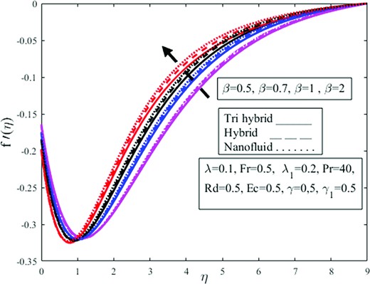
Impact of Casson fluid parameter |$\beta $| on the radial velocity profile |$f^{\prime}( \eta )$|.
Figures 4–15 are constructed to check the impact of the dimensionless governing parameters like fluid parameter |$\ \beta $|, buoyancy ratio parameter |$\ \lambda $|, Darcy–Forchheimer parameter |$Fr$|, porosity parameter |${\lambda }_1$|, radiation parameter |$\ Rd$|, Prandtl number |$\ Pr$|, Eckert number |$\ Ec$|, and velocity slip parameter |$\ \gamma \ $| are elucidated on the dimensionless velocity |$( {f^{\prime}( \eta ),\ g( \eta )} )$| and temperature |$( {\theta ( \eta )} )$| profiles. The solid, solid-dashed, and dotted lines are plotted to examine the effects on ternary hybrid, hybrid, and nanofluid. The influence of the parameter |$\ \beta \ $| upon radial |$\ f^{\prime}( \eta )$| and azimuthal |$g( \eta )$| velocities are captured in Figs 4 and 5. For increasing values of the parameter |$\ \beta $|, the radial velocity appears to be decreasing near the wall but increases as the distance from the wall is increased. The boundary layer thickness is reduced as the parameter |$\ \beta \ $| is increased. Physically the Casson fluid parameter resists the fluid flow, and the boundary layer thickness is reduced. Physically the Casson fluid parameter |$\beta $| determines the fluid viscosity. Physically shear thickening behavior is observed owing to magnification in |$\beta $| which diminishes the fluid velocity. The shear thickening behavior of the fluid resists the fluid motion. Besides, the function of nanoparticles is to enhance the fluid temperature and diminishes the fluid viscosity which amplifies |$\beta $| and lessens the fluid velocity. Upon comparing non-Newtonian Casson fluid to Newtonian fluid, the velocity magnitude is higher. The effects of the parameter |$\ \beta \ $| on the radial velocity are greater for the nanofluid. Besides, the azimuthal velocity in Fig. 5 demonstrates the opposite effects for Casson fluid parameter |$\ \beta \ $| than the radial velocity in Fig. 4. It is observed from Fig. 4 that the fluid is moving away from the wall in the upward direction owing to magnification in Casson fluid parameter |$\beta $| from 0.5 to 2. The thickness of the momentum boundary layer amplifies under magnification in |$\beta $|. The concentration of fluid diminishes under amplification in the volume fraction of nanoparticles. It is observed that the radial velocity amplifies more in the case of nanofluid in contrast to di-hybrid and tri-hybrid nanofluid. Physically an amplification in |$\beta $| and volume fraction of nanoparticles produces extensive heat which is absorbed by the surface of the cone and the radius of the cone surface amplifies fluid moving easily over the surface and radial velocity field amplifies but azimuthal velocity |$g( \eta )$| diminishes on the other hand as shown in Fig. 5. Figure 6 is intended to inspect the |$f^{\prime}( \eta )$| profile against parameter |$\ \lambda .\ $|The higher buoyancy ratio parameter causes a reduction in the radial velocity profile. Bioconvection physically restricts the upward motion of the solid particles that originate in nanofluid for a certain buoyancy effect; however, the fluid meets resistance for higher buoyancy estimations, causing a decrement in fluid velocity. The decrease for the ternary hybrid is prominent. The physical buoyancy ratio parameter is the ratio of the Grashoff number to the square of the Reynolds number. Grashoff number is the ratio of buoyant forces to viscous forces and Reynolds number is the ratio of viscous forces to inertial forces. Physically, it is observed that the viscous forces dominate on the behalf of a magnification in |$\lambda $| which provides resistance to the fluid flow and amplifies the fluid viscosity which diminishes the radial velocity |$f^{\prime}( \eta ).$| It is obvious from the figure that magnification in |$\lambda $| from 0.5 to 2 amplifies viscosity and fluid is approaching the vertical wall and this downward approaching trend is more dominant in the case of ternary fluid in contrast to di-hybrid and mono nanofluid. The |$f^{\prime}( \eta )$| and |$\ g( \eta )$| profiles against parameter |${F}_r$| are encapsulated in Figs 7 and 8. It is evidenced from these figures that the radial velocity near the wall and azimuthal velocity are in a reducing trend for higher estimations of the Darcy–Forchheimer parameter. The rise in the Darcy number amplifies the resistive forces throughout this phase, and as a result, fluid velocities decrease. However, this trend is in the opposite direction for radial velocity when it goes away from the wall. The Darcy–Forchheimer is observed to equally influence the ternary hybrid, hybrid, and nanofluid. Physically Darcy’s law is valid for the case of laminar flow having a low Reynolds number and utilized where the velocity of the fluid is low. Forchheimer modifies the Darcy law by adding the square of the velocity factor known as the Darcy–Forchheimer term and utilized where high velocity is required. It is observed from the figure that the velocity of the fluid is approaching the vertical wall at the start but approaching away from the vertical wall in after upward direction due to amplification in the Forchheimer parameter |${F}_r$| from 0.5 to 1.4. The fluid is moving quickly over the cone which amplifies radial velocity |$f^{\prime}( \eta )$| and azimuthal velocity |$g( \eta )$| acting in the direction of rotation of fluid amplifies due to the fast rotation of the fluid. Ternary hybrid nanofluid amplifies more in contrast to mono and dihybrid nanoparticles owing to magnification in |${F}_r.$| Figures 9 and 10 show the |$f^{\prime}( \eta )$| and |$\ g( \eta )$| profiles versus parameter |${\lambda }_1.\ $| From these figures, the higher estimations of |${\lambda }_1$| causes the radial velocity in Fig. 9 near the wall and the azimuthal velocity |$\ g( \eta )$| in Fig. 10 decreases but increases away from the wall, radial velocity increases. It is well established that the velocity is inversely proportional to the porosity phenomenon. Physically an amplification in the viscosity phenomenon is affected by the positive variation in the porosity parameter and is inversely related to the permeability of the medium which is responsible for a decrement in fluid velocity. Physically, increasing the porosity parameter enhances the resistance of the porous material, causing the velocity components to decrease. The ternary hybrid in the radial velocity profile is greater than others, but there is an opposing behavior in azimuthal velocity. From Fig. 10, it is observed that amplification in nanofluid is more dominant in contrast to ternary as well as di-hybrid nanofluid, but the rotating factor of the fluid diminishes owing to magnification in |${\lambda }_1$| which declines nanofluid more quickly in comparison to dihybrid as well as trihybrid nanofluids as shown in Fig. 10.
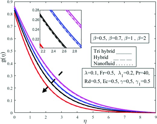
Effect of Casson fluid parameter |$\beta $| on azimuthal velocity profile |$g( \eta ).$|
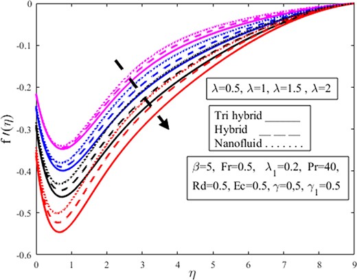
Influence of buoyancy ratio parameter |$\lambda $| on the radial velocity profile |$f^{\prime}( \eta )$|.
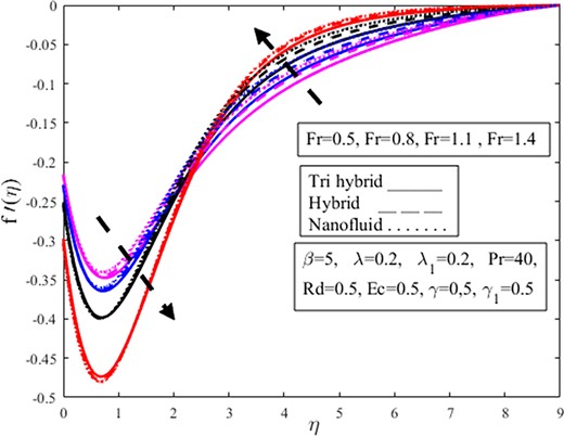
Effect of Forchheimer number |$Fr$| on the radial velocity profile |$f^{\prime}( \eta )$|.
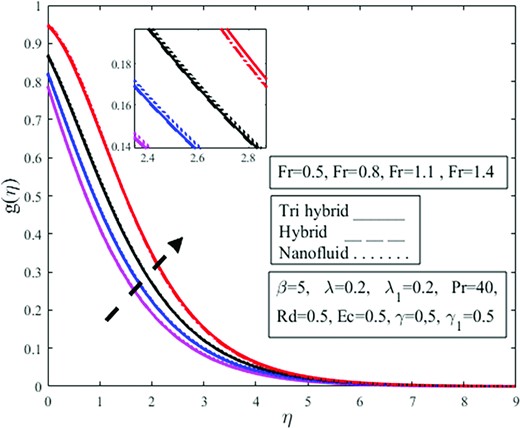
Effect of Forchheimer number |$Fr$| on azimuthal velocity profile |$g( \eta )$|.
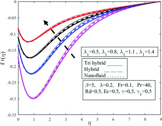
Effect of porosity parameter |${\lambda }_1$| on the radial velocity profile |$f^{\prime}( \eta )$|.
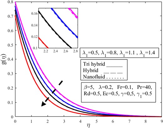
Impact of porosity parameter |${\lambda }_1$| on azimuthal velocity profile |$g( \eta )$|.
The impact of |$Rd$|on |$\theta ( \eta )$| profile is determined in Fig. 11. It appears to rise as |$Rd$| enhances. According to the physical principle, the mean absorption coefficient falls as the radiation parameter upsurges resulting in tremendous heat being produced toward the fluid, resulting in the temperature growing. The growth for the ternary hybrid is on the higher side than that of others. The addition of nanoparticles together with thermal radiation amplifies the fluid temperature. The random collision between particles is due to the magnification in |$Rd$| which amplifies the temperature field. Radiation is one of the modes of heat transfer with the remaining two being conduction and convection. Physically thermal radiation is used where more temperature difference is required having industrial applications in the cleaning of surgical pieces of equipment, combustion reactors, nuclear reactors polymer production, etc. It is well established that the insertion of nanoparticles in the base enhances the thermal conductivity of the fluid. From Fig. 11 it is observed that the temperature field amplifies under amplification in thermal radiation |$Rd$| and fluid is moving away from the vertical wall in the upward direction. It is observed from the figure that temperature amplifies more in the case of tri-hybrid nanoparticles in comparison to di-hybrid and mono nanoparticles. The impression of the parameter |$\ Pr\ $| on the profile |$\ \theta ( \eta )$| are exemplified in Fig. 12. For higher |$Pr$|, the temperature profile appears to be decreasing. The Prandtl number demonstrates the relationship between momentum diffusivity to thermal diffusivity. An enlargement in the Prandtl number implies a reduction in thermal diffusivity. Physically in heat transport phenomena, the parameter |$\ Pr\ $| helps to govern the relative thicknesses of the thermal and momentum boundary layer. The thermal boundary layer thickness is reduced as |$Pr$| rises, causing a drop in the temperature profile. The change in Prandtl is also linked with viscosity change and viscosity is inversely proportional to the temperature. That is why an amplification in viscosity escalates the |$Pr$| and diminishes the temperature field. Also, this drop is on the extreme side of the nanofluid than others. That is why a magnification in |$Pr$| diminishes temperature inside the fluid which diminishes the nanoparticle effect on the fluid flow and this decrement is more dominant in the case of mono nanofluids in contrast to di and ternary hybrid nanofluids. |$Ec\ $| parameter versus |$\theta ( \eta )$| profile is depicted in Fig. 13. The temperature profile is shown to be decreasing. Eckert number relates to the kinematic energy and enthalpy variation of the boundary layer. Increasing the parameter |$\ Ec\ $| causes a substantial decrement in the velocity. A rising |$Ec$| induces a growth for the temperature and momentum, but this deviates from the norm, revealing a monotonous degradation of the wall. However, the overwhelming influence of heat flux boundary conditions and species. Also, the reduction for nanofluid is larger than others. Physically Eckert number is used to assess whether or not the role of momentum energy being converted to thermal energy has a major impact on the flow. In conditions where high speeds are involved, the importance of this impact cannot be overstated. It is well established that amplification in volume fraction of nanoparticles provides resistance to the fluid flow and amplifies phenomenon which diminishes momentum and energy, and this energy is not effectively transformed into heat energy which diminishes temperature phenomenon inside the fluid and abates temperature field |$\theta ( \eta ).$|
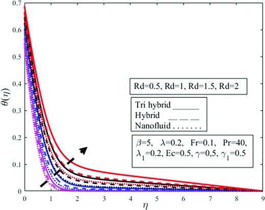
Effect of thermal radiation parameter |$Rd$| on temperature profile |$\theta ( \eta )$|.
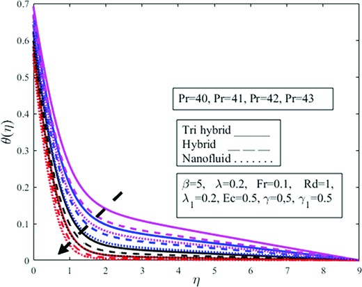
Effect of Prandtl number |$Pr$| on temperature profile |$\theta ( \eta )$|.

Impact of Eckert number |$Ec$| on temperature profile |$\theta ( \eta )$|.
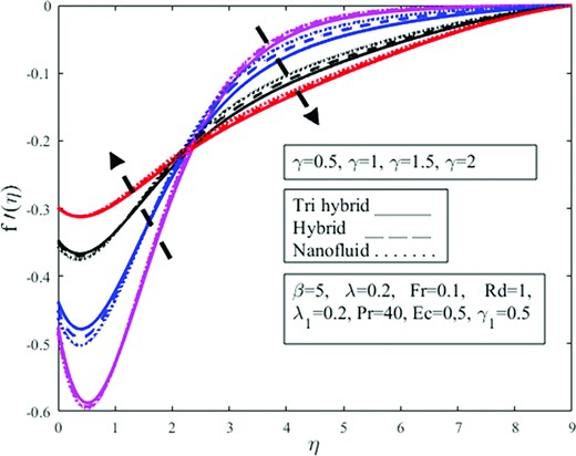
The purpose of Figs 14 and 15 are to see how the parameter |$\ \gamma \ $| influences the dimensionless profiles |$\ f( \eta )$| and |$\ g( \eta )$|. The rising velocity slip parameter |$\gamma $|makes the velocity profiles curve decay. Due to the slippage condition, the velocity of the fluid is not uniform when moving over the slipping surface. Shear thickening behavior is significant when the slip parameter is augmented. Physically fluid flows over a slippery surface and cannot move quickly and becomes more viscous, which causes the velocity to depreciate. When a slip appears, the cone’s velocity is not similar to that of the flow velocity near the cone. The distortion is partially transferred to the fluid, resulting in lower velocity profiles. Fluid is approaching the vertical wall but gradually moving away from the vertical wall in the upward direction as a result of magnification in |$\gamma $| from 0.5 to 2 which amplifies |$f( \eta )$| moreover, shear thickening is observed which depreciates the rotating aspect of the fluid flow and diminishes azimuthal velocity |$g( \eta )$|. The ternary hybrid near the wall is significantly larger than the other, but this pattern goes reversed away from the wall.
Effect of velocity slip condition |$\gamma $| on radial velocity |$f^{\prime}( \eta )$|.
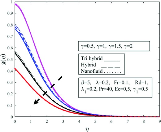
Impact of velocity slip condition |$\gamma $| on azimuthal velocity profile |$g( \eta )$|.
Figure 16 highlights the contour plot for velocity distribution against |$\lambda .$| Enhancing the estimations of |$\lambda $| decelerates the velocity distribution. The behavior of velocity distribution against |$\beta $| is demonstrated in Fig. 17 in the form of a contour plot. The velocity distribution amplifies with the growing estimations of |$\beta .$| The contour characteristics of azimuthal velocity are portrayed in Fig. 18 against |$Fr.$| The azimuthal velocity is a growing function due to higher estimations of |$Fr.$| Figure 19 depicted the contour justifications of azimuthal velocity against |${\lambda }_1.$| One can see that the azimuthal velocity distribution is de-escalating with the climbing estimations of |${\lambda }_1.$| Figure 20 presented the impact of the Eckert number on the temperature profile in the form of a contour graph. The temperature profile is diminished against higher estimations of the Eckert number. The contour influence of the Prandtl number on the temperature profile is shown in Fig. 21. One can notice that the temperature distribution is de-increment with the incrementing estimations of the Prandtl number.
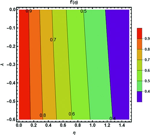
Contour plot of velocity slip parameter |$\lambda $| against radial velocity field.
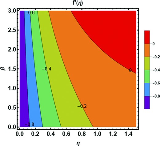
Contour plot of Casson fluid parameter |$\beta $| against radial velocity field.
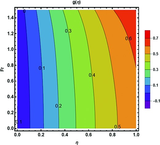
Contour plot of Forchheimer number |$Fr$| against azimuthal velocity field.
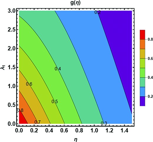
Contour plot of the dimensionless porosity parameter |${\lambda }_1$| against azimuthal velocity field.
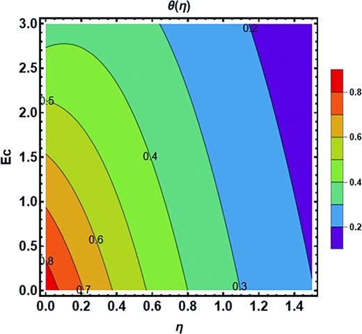
Contour plot of dimensionless Eckert number |$Ec$| against temperature field.
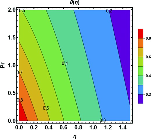
Contour plot of dimensionless Prandtl fluid parameter |$Pr$| against temperature field.
The numerical values of the interesting physical quantities for various ranges of the pertinent parameters are calculated in Table 5. A thorough comparison is constituted for hybrid and ternary hybrid nanofluids. This table reveals that the skin friction coefficients diminish more in the case of trihybrid nanofluids for parameters |$\lambda $|, |$Fr$|, and |${\lambda }_1$| in comparison to a di-hybrid nanofluid. The heat transfer rate amplifies in the case of trihhybrid nanofluid for |$\lambda $|, |$Fr$|, and |${\lambda }_1$| in contrast to a di-hybrid nanofluid. It is noticed that the surface drag diminishes more quickly in the case of tri-hybrid nanofluid for the case of dimensionless parameters |$Pr$|, |$Rd$|, |$Ec$|, |$\gamma $|, and |${\gamma }_1$| in comparison to di-hybrid nanofluid but reverse behavior is reported in the case of heat transfer phenomenon where insertion of tri-hybrid nanoparticles in the base fluid in the case of distinguished sundry parameters |$Pr$|, |$Rd$|, |$Ec$|, |$\gamma $|, and |${\gamma }_1$| amplifies the Nusselt heat transfer phenomenon in contrast to a di-hybrid nanofluid.
The numerical values of the skin friction coefficient and Nusselt number are subjected to the governing parameters.
| Dimensionless parameters | Hybrid nanofluid | Ternary hybrid nanofluid | |||||||||||
|---|---|---|---|---|---|---|---|---|---|---|---|---|---|
| |$\lambda $| | |$Fr$| | |${\lambda _1}$| | |$Pr$| | |$Rd$| | |$Ec$| | |$\gamma $| | |${\gamma _1}$| | |$C{f_x}Re_x^{\frac{1}{2}}$| | |$C{f_y}Re_x^{\frac{1}{2}}$| | |$N{u_x}Re_x^{\frac{{ - 1}}{2}}$| | |$C{f_x}Re_x^{\frac{1}{2}}$| | |$C{f_y}Re_x^{\frac{1}{2}}$| | |$N{u_x}Re_x^{\frac{{ - 1}}{2}}$| |
| 0.1 | 1 | 0.1 | 39 | 0.5 | 1.5 | 0.5 | 0.5 | 1.8356 | 1.4256 | 2.6541 | 1.7857 | 1.4123 | 3.3456 |
| 0.3 | 1.7654 | 1.4132 | 2.6231 | 1.7253 | 1.3901 | 2.8756 | |||||||
| 0.5 | 1.7254 | 1.4098 | 2.6015 | 1.6950 | 1.3804 | 2.7149 | |||||||
| 1.1 | 1.9536 | 1.3205 | 3.8041 | 1.9015 | 1.2711 | 3.9542 | |||||||
| 1.2 | 1.9021 | 1.2651 | 3.8246 | 1.8531 | 1.2021 | 4.0153 | |||||||
| 1.3 | 1.8536 | 1.2031 | 3.8571 | 1.8123 | 1.1736 | 4.6221 | |||||||
| 0.3 | 1.8756 | 1.6173 | 2.9654 | 1.6034 | 1.5023 | 2.7118 | |||||||
| 0.5 | 1.7432 | 1.5059 | 2.6750 | 1.4145 | 1.4131 | 2.4553 | |||||||
| 0.7 | 1.6578 | 1.4157 | 2.3119 | 1.2098 | 1.3756 | 2.1716 | |||||||
| 40 | 1.8115 | 1.4147 | 2.6563 | 1.5013 | 1.3190 | 3.3785 | |||||||
| 41 | 1.9345 | 1.2003 | 2.6756 | 1.7654 | 1.1231 | 3.4498 | |||||||
| 42 | 2.1217 | 1.1963 | 2.7432 | 1.9865 | 1.0123 | 3.6823 | |||||||
| 1 | 1.8154 | 1.6231 | 3.1118 | 1.4201 | 1.3132 | 4.2243 | |||||||
| 1.5 | 1.9235 | 1.5784 | 3.2543 | 1.5024 | 1.2367 | 4.4398 | |||||||
| 2 | 2.0745 | 1.4572 | 3.3953 | 1.6167 | 1.1904 | 4.6541 | |||||||
| 1.7 | 1.8976 | 1.5413 | 2.6534 | 1.5242 | 1.2596 | 3.4546 | |||||||
| 1.9 | 1.7346 | 1.4561 | 2.8756 | 1.4345 | 1.1177 | 3.7851 | |||||||
| 2.1 | 1.6677 | 1.3274 | 3.0315 | 1.3137 | 1.0234 | 4.2468 | |||||||
| 0.7 | 1.9192 | 1.5566 | 3.9933 | 1.8013 | 1.2277 | 2.9186 | |||||||
| 0.9 | 1.7082 | 1.4164 | 3.5254 | 1.6246 | 1.1218 | 2.6324 | |||||||
| 1.1 | 1.5341 | 1.3956 | 2.9197 | 1.4532 | 1.0596 | 2.3115 | |||||||
| 0.7 | 1.7231 | 1.4768 | 2.9897 | 1.6135 | 1.2143 | 3.9765 | |||||||
| 0.9 | 1.6415 | 1.3562 | 2.7215 | 1.5125 | 1.1456 | 3.5274 | |||||||
| 1.1 | 1.5230 | 1.2876 | 2.5246 | 1.4163 | 1.0214 | 3.2143 | |||||||
Table 5 is designed to present the percentage analysis for the case of various sundry parameters in the case of heat transfer Nusselt number. The table represents the difference in the heat transfer rate of ternary hybrid nanofluid minus dihybrid nanofluid by ternary hybrid nanofluid multiplied by a hundred percent. The obtained outcomes are mentioned in Table 6 given below.
Percentage change in heat transfer under magnification in sundry parameters.
| Parameters | Hybrid nanofluid | Tri-hybrid nanofluid | Percentage change | ||||
|---|---|---|---|---|---|---|---|
| |$Pr$| | |$Rd$| | |$Ec$| | |$\gamma $| | |${\gamma _1}$| | |$N{u_x}Re_x^{\frac{{ - 1}}{2}}$| | |$N{u_x}Re_x^{\frac{{ - 1}}{2}}$| | |$\Big| {\frac{{{{( {Nux} )}_{ter}} - {{( {Nux} )}_{hyb}}}}{{{{( {Nux} )}_{ter}}}}} \Big| \times 100\% $| |
| 39 | 0.5 | 1.5 | 0.5 | 0.5 | 2.6541 | 3.3456 | 20.6% |
| 40 | 2.6563 | 3.3785 | 21.3% | ||||
| 41 | 2.6756 | 3.4498 | 23.5% | ||||
| 42 | 2.7432 | 3.6823 | 25.2% | ||||
| 1 | 3.1118 | 4.2243 | 26.2% | ||||
| 1.5 | 3.2543 | 4.4398 | 27.3% | ||||
| 2 | 3.3953 | 4.6541 | 28.4% | ||||
| 1.7 | 2.6534 | 3.4546 | 23.2% | ||||
| 1.9 | 2.8756 | 3.7851 | 24.0% | ||||
| 2.1 | 3.0315 | 4.2468 | 28.6% | ||||
| 0.7 | 3.9933 | 2.9186 | 36.8% | ||||
| 0.9 | 3.5254 | 2.6324 | 25.5% | ||||
| 1.1 | 2.9197 | 2.3115 | 20.2% | ||||
| 0.7 | 2.9897 | 3.9765 | 25.8% | ||||
| 0.9 | 2.7215 | 3.5274 | 22.8% | ||||
| 1.1 | 2.5246 | 3.2143 | 21.4% | ||||
6. Conclusions
A novel mathematical ternary hybrid nanofluid flow model bounded by a porous cone is developed to obtain better heat transfer results, with thermal radiation and viscous dissipation. The flow dynamics are modeled in terms of the non-linear PDEs, and later, a similar solution is obtained through the assistance of KBM. Thus, from comprehensive exploration, the following conclusion is observed. The article is novel in the sense that the effect on ternary hybrid nanofluid moving subjected to a rotating cone having a slippery surface with effects like Maxwell velocity and Smoluchowski temperature slip boundary conditions are not explored yet in the existing literature. Fluid flow over a rotating with porosity and Darcy–Forchheimer effects are various practical industrial applications like cone clutch, cone bottom tanks storing fluid, small cone crushers, air atomizing nozzles, etc. The important outcomes of the present study are enumerated below.
The Casson fluid parameter |$\beta $| magnifies the shear thickening phenomenon which brings about an abatement in the velocity profile |$f^{\prime}( \eta )$|.
Darcy–Forchheimer |$Fr$| effect provides resistance to fluid flow and diminishes |$f^{\prime}( \eta ).$|
Viscosity and temperature are inversely related. An increase in viscosity depreciates the velocity and amplifies the temperature as shown in the obtained results.
Viscosity of fluid amplifies due to the buoyancy effect |$\lambda $| which reduces the fluid flow and diminishes the velocity profile|$\ f^{\prime}( \eta ).$|
The azimuthal velocity |$\ g( \eta )$| is somehow related to the rotating phenomenon. A positive variation in the Casson fluid parameter amplifies fluid viscosity and fluid is unable to rotate easily which diminishes azimuthal velocity |$\ g( \eta )$|. The permeability of fluid decreases due to magnification in |${\lambda }_1$| which provides resistance to fluid flow and rotational effect of the fluid which decreases azimuthal velocity|$\ g( \eta ).$|
The temperature |$\ \theta ( \eta )$| is escalating for the parameter of thermal radiation which is used where a large temperature is required having enormous applications in nuclear reactors, polymer production combustion reactors, etc. A positive variation in |$\ Rd\ $| amplifies the thermal conductivity of fluid which amplifies |$\theta ( \eta ).$|
Physically momentum energy is not converted efficiently into thermal energy because the viscosity of fluid increases owing to an amplification in |$Ec$| which diminishes fluid temperature.
Thermal conductivity amplifies more and the average kinetic energy of molecules inside the fluid amplifies which amplifies the overall temperature of the fluid this change is more dominant in the case of agglomerative tri nanoparticles in comparison to di-hybrid and mono nanoparticles.
The velocity slip parameter decreases the velocity field. Physically the velocity of the fluid and surface are not the same and due to the roughness of the surface, fluid cannot move easily over the surface which diminishes fluid velocity.
The temperature field diminishes owing to magnification in the Smoluchowski temperature slip parameter because the temperature of the fluid and the temperature of the cone surface over which the fluid is moving is not the same which abates the temperature field.
Heat transfer rate amplifies more 26.8% in the case of Eckert number having value |$Ec = 2.1\% $| but diminishes heavily in the slip parameter having value |$\gamma = 0.7$|.
The heat transfer rate diminishes from 25.8% to 21.4% in the case of magnification in the temperature slip parameter |${\gamma }_1 = 0.7$|–1.1.
Nusselt number amplifies by 26.2–28.4% because of magnification in radiation parameter |$Rd = 1$|–2.
It can be said that in the near future, we are currently working on extending the current concept in this study to include the main ideas in the following valuable papers (Aziz et al., 2020; Hussain & Jamshed, 2021; Jamshed et al., 2021a, b, c, d; Wang et al., 2021, 2023a, b, c).
Acknowledgement
The authors extend their appreciation to the Deanship of Scientific Research at King Khalid University for funding this work through large group Research Project under grant number RGP2/251/44.
Data availability
Manuscript has no associated data.
Conflict of interest statement
There is no conflict of interest.
