


Abstract
Genomic information has a limited dimensionality (number of independent chromosome segments [Me]) related to the effective population size. Under the additive model, the persistence of genomic accuracies over generations should be high when the nongenomic information (pedigree and phenotypes) is equivalent to Me animals with high accuracy. The objective of this study was to evaluate the decay in accuracy over time and to compare the magnitude of decay with varying quantities of data and with traits of low and moderate heritability. The dataset included 161,897 phenotypic records for a growth trait (GT) and 27,669 phenotypic records for a fitness trait (FT) related to prolificacy in a population with dimensionality around 5,000. The pedigree included 404,979 animals from 2008 to 2020, of which 55,118 were genotyped. Two single-trait models were used with all ancestral data and sliding subsets of 3-, 2-, and 1-generation intervals. Single-step genomic best linear unbiased prediction (ssGBLUP) was used to compute genomic estimated breeding values (GEBV). Estimated accuracies were calculated by the linear regression (LR) method. The validation population consisted of single generations succeeding the training population and continued forward for all generations available. The average accuracy for the first generation after training with all ancestral data was 0.69 and 0.46 for GT and FT, respectively. The average decay in accuracy from the first generation after training to generation 9 was −0.13 and −0.19 for GT and FT, respectively. The persistence of accuracy improves with more data. Old data have a limited impact on the predictions for young animals for a trait with a large amount of information but a bigger impact for a trait with less information.
Introduction
The addition of genomic information to routine genetic evaluations reduced generation interval and increased the accuracy of genomic estimated breeding value (GEBV), defined as the correlation between true and estimated breeding values (VanRaden et al., 2009). These factors are the main forces driving the increase in the rate of genetic gain over time (VanRaden, 2008; García-Ruiz et al., 2016). Genomic information helps to identify the best young animals accurately even before phenotypes are recorded; therefore, it is of interest to determine the accuracy of GEBV for generations without new data recording and the magnitude of decay of accuracy over time. The selection of novel traits and traits difficult to measure is mainly dependent on the accuracies of GEBV. For example, milking speed and temperament have shown promising genetic progress due to genomics (Chen et al., 2020). Initial studies in genomic selection showed great persistence in the accuracy of genomic predictions over time. The results from the study of Meuwissen et al. (2001) showed marginal decay in accuracy with a decrease from 0.84 to 0.72 over five new generations without phenotypes. This created initial excitement for the potential of selection with genomic information; however, the parameters of the simulated population cannot be compared with present-day commercial livestock populations. In the simulation, there was no selection, and only a few major genes explained the additive genetic variance of the trait. Under strong selection, steep decay in accuracy occurs (Muir, 2007). In small, simulated populations, Muir (2007) found that the accuracy of GEBV decays more rapidly than expected when under strong selection compared with random selection.
We hypothesize that the decay will be minimized even under selection if enough phenotypes and genotypes are available to represent the population structure. The reason is that a limited number of independent chromosome segments (Me) theoretically explain the additive genetic variance in a population (Pocrnic et al., 2016a). Therefore, if enough information exists to precisely estimate the effects of Me, the additive genetic variance can be explained, and accuracies will be adequate and stable over time. The number of Me is dependent on the effective population size (Ne) and genome length (L) (Stam, 1980). Pocrnic et al. (2016a) showed that the optimal amount of Me can be estimated by computing the number of eigenvalues that explain a certain proportion of variation in the genomic relationship matrix (GRM), which is used in genomic best linear unbiased prediction (GBLUP; VanRaden, 2008) and single-step GBLUP (ssGBLUP; Aguilar et al., 2010). This creates a threshold for the amount of information that is nonredundant, that is, information that can increase accuracy, and the amount of which new data no longer increases the accuracy. Hence, the GRM has a limited dimension. Whereas NeL eigenvalues explain most of the information, no new information is added after 4NeL (Stam, 1980; Pocrnic et al., 2016a). Goddard (2009) showed that accuracy is inversely related to Ne. As Ne increases, accuracy decreases. It is estimated that genome lengths for pigs range from 18 to 23 Morgan (Rohrer et al., 1994; Archibald et al., 1995; Marklund et al., 1996; Tortereau et al., 2012), and Ne ranges from 55 to 113 (Welsh et al., 2009; Uimari and Tapio, 2011; Pocrnic et al., 2016b). Pocrnic et al. (2016b) found that 5,000 segments explain approximately 98% of the variation in commercial pig populations. With enough data relative to the independent chromosome segments, high accuracy could be achieved. Additionally, if the segments are well estimated, there should be less decay of predictivity under the additive model even under selection.
The inverse of the GRM can be obtained by recursion on a group of animals (Faux et al., 2012; Misztal et al., 2014), with the optimal group size equal to the dimensionality of the genomic information (Misztal, 2016). The recursion means that the breeding value of any animal can be estimated with near-perfect accuracy from the exact breeding values of 4NeL other animals. Bradford et al. (2017) showed by simulation that the accuracy of GEBV was the same whether the recursion was based on animals from the last generation or a distant generation. Their results suggest that, under the additive model, the persistence of genomic evaluations is very high if the reference population includes 4NeL animals with high accuracy or equivalent.
Although accuracy is dependent on the proportion of variance explained by the eigenvalues of the GRM, the distribution of eigenvalues is not consistent, and a small percentage of the largest eigenvalues explain the majority of the genetic variation (Pocrnic et al., 2019). Additionally, the animals necessary to explain the largest eigenvalues carry almost the same genomic information. Hence, selection by GBLUP-based models occurs on clusters of independent chromosome segments, not individual chromosome segments (Pocrnic et al., 2019). In pig populations, the segments can be well estimated if there are around 5,000 animals available with very high accuracy (e.g., theoretical EBV accuracy based on prediction error variance) or an equivalent number of animals with less accuracy. Despite a large amount of data available, the decay will be more dramatic if genomic selection induces faster epistatic changes (Huang and Mackay, 2016). Epistatic interactions between genes may reduce the value of old data, and epistatic effects may be unstable across populations because of the fluctuation in allele frequencies (Varona et al., 2018).
With the commercial pig production systems and population structure, the Ne and the Me are small. The purpose of this study is to determine how accuracy and the decay in accuracy are affected by the quantity of data available, the heritability of the trait, and removing data from ancestral generations. With genotypes now available for many generations in pigs, reliable predictions for generations without new phenotype recordings may be possible.
Materials and Methods
Animal Care and Use Committee approval was not needed because information was obtained from preexisting databases.
Data
Data for animals born between 2008 and 2020 were provided by Smithfield Premium Genetics (Rose Hill, NC). The population consisted of 273,382 animals, of which 55,118 were genotyped or imputed to the 50k single-nucleotide polymorphism (SNP) panel for autosomal markers only. Quality control removed SNP with minor allele frequency lower than 0.05, SNP and animals with call rates lower than 0.9, SNP with the difference between expected and observed frequency of heterozygous greater than 0.15 (departure from the Hardy–Weinberg equilibrium), and animals with parent-progeny Mendelian conflicts. After quality control, 39,263 SNPs remained for 53,147 genotyped animals.
The dataset consisted of 27,669 records for a repeated fitness trait (FT) related to prolificacy from 13,883 animals and 161,495 records for a single growth trait (GT). The population consisted of 11 generations. Generations were constructed by tracing the population back to the oldest animals with no recorded parents. These animals were considered generation 1, and their progeny, grand-progeny, and great-grand-progeny were placed in generations 2, 3, and 4, respectively, and continued until generation 11. The birth year of the animals without parent records was considered when joining the successions to be more precise and to account for the age variation of animals without parent records. Table 1 presents the number of animals with genotypes, phenotypes, and pedigree per generation.
Number of animals in the pedigree, genotyped animals, and records for GT and FT per generation
| Generation | Pedigree | Genotypes | GT | FT |
|---|---|---|---|---|
| 1 | 758 | 214 | 658 | 1,991 |
| 2 | 12,513 | 384 | 4,767 | 2,098 |
| 3 | 15,190 | 831 | 7,697 | 3,447 |
| 4 | 29,017 | 1,929 | 16,491 | 3,753 |
| 5 | 38,316 | 2,775 | 23,211 | 4,302 |
| 6 | 42,476 | 6,158 | 26,474 | 4,278 |
| 7 | 44,363 | 10,769 | 28,260 | 3,348 |
| 8 | 39,082 | 11,345 | 25,002 | 2,290 |
| 9 | 27,445 | 8,636 | 16,989 | 1,435 |
| 10 | 17,084 | 6,149 | 8,762 | 570 |
| 11 | 7,138 | 3,957 | 3,184 | 157 |
Model and analyses
Variance components were estimated using AIREMLF90 (Misztal et al., 2014) without genomic information. The heritabilities were 0.21 and 0.06 for GT and FT, respectively, with standard errors less than 0.01. GEBVs were computed using ssGBLUP (Aguilar et al., 2010). Two single-trait models were used in the analyses :
where G was constructed using the first method of VanRanden (2008), then 95% of G was blended with 5% of the pedigree relationship matrix for genotyped animals (A22), and finally tuned so that the means of the diagonal and off-diagonal elements were similar to those of A22 (Chen et al., 2011). The allele frequencies used to compute G were calculated based on all genotyped animals in the dataset.
In this study, the accuracy and dispersion of GEBV were estimated with the linear regression (LR) method (Legarra and Reverter, 2018). This method uses two datasets, namely the whole dataset and the partial dataset, hereinafter denoted with the subscripts w and p, respectively. The former contains all the available phenotypes up to a certain time t, whereas the latter contains phenotypes up to a time period before t. The focal individuals, that is, the individuals for whom the accuracy of GEBV will be estimated, are defined as the genotyped animals with phenotypes in the whole dataset but without in the partial dataset.
To investigate the impact of the amount of data on the accuracy of GEBV for focal individuals, GEBV were sequentially estimated by changing the definition of focal individuals and partial datasets using a sliding approach based on generation. Figure 1 shows four definitions of focal groups that included generations 5 to 9, 6 to 9, 7 to 9, and 8 and 9. Accuracy and dispersion were then calculated separately for each generation of focal individuals. Additionally, to investigate the impact of ancestral data, four partial datasets were created for each focal group: 1) the ancestral group: contained all the ancestors of the focal individuals, 2) the 3-generation group: consisted of the ancestors up to the great-grandparents of the focal individuals, 3) the 2-generation group: included the grandparents and parents of the focal individuals, and 4) the 1-generation group: contained only the parents of the focal individuals. A total of 16 different combinations of groups of focal individuals and partial datasets were created (Figure 1).

Scheme for partial datasets and focal animals. The four partial dataset groups include ancestral, 3-, 2-, and 1-generation subsets. In each scenario, the genomic and pedigree information is included for all animals and remains unchanged, but only phenotypes exist for animals in the partial dataset. Generations are not grouped for the focal animals, and accuracies are calculated for each generation separately.
The benchmark for each validation, that is, GEBVw, remained unchanged, whereas GEBVp was updated as the partial datasets were modified. Due to the lack of phenotypes and genotypes in generations 10 and 11, these animals were removed from all analyses as they were incomparable with the other validation generations. Accuracies were estimated for each generation in each set of focal individuals using: (Legarra and Reverter, 2018; Macedo et al., 2020b), where is the average inbreeding coefficient among focal individuals in a specific generation and is the estimated additive genetic variance of the population. Inbreeding coefficients for each animal were calculated with a recursive method based on pedigree using INBUPGF90 (Aguilar and Misztal, 2008). The slope of the regression of on is used to assess the dispersion of partial GEBV and is equal to . The primary purpose of this research was to compare accuracies over time with varying amounts of ancestral data for two traits of differing heritabilities; therefore, other statistical parameters were not used. Accuracy and dispersion are well researched and logical to use as a function over time (Macedo et al., 2020a). Additional statistics proposed by the LR method have not been widely tested as a function of time. Including those values would output uninterpretable comparisons and should be further researched.
Results and Discussion
Figures 2 and 3 show the accuracy for GT and FT over time using the partial datasets belonging to each group. When comparing traits, GT had higher accuracy and less decay in accuracy over time compared with FT. For example, when considering the partial dataset composed of generations 1 to 4 from the ancestral group, the accuracy decreased from 0.55 in generation 5 to 0.42 in generation 9 for GT (Figure 2A), and from 0.46 to 0.22 for FT (Figure 3A), respectively. These results are expected and agree with those from Muir (2007) since GT has higher heritability than FT, and low heritability traits require a large number of records to achieve high accuracy; FT had about one-sixth of the records compared with GT.

Accuracy over time with four partial dataset groups for GT. The partial datasets are updated over time, increasing a generation of data for the ancestral groups (A) and adding a recent generation of data while removing the oldest generation of data for 3-, 2-, and 1- generation subsets (B, C, and D, respectively). Accuracy is calculated for each generation separately, beginning with the first generation following the partial dataset and ending at generation 9.
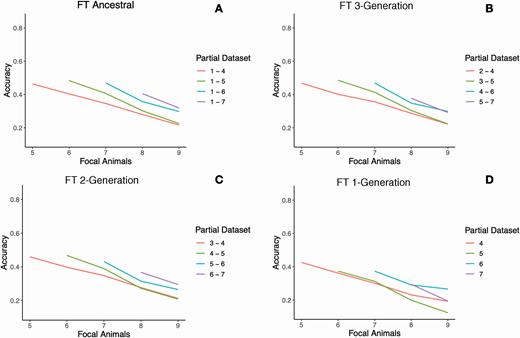
Accuracy over time with four partial dataset groups for FT. The methods are the same as in Figure 2.
Persistence for both traits can be inferred by observing the initial and final accuracy for each line in Figures 2 and 3. The slopes for FT are greater in magnitude than the slopes for GT, meaning that the latter showed more persistence. The differences in persistence between the two traits may be explained by the heritability and the amount of phenotypic information. Roughly, the amount of information in this study can be approximated as accuracies of hypothetical 5,000 (4NeL) sires with as many progeny as the number of animals with records and with progeny equally distributed per sire. For a trait with 32 progeny per sire and heritability of 0.21, the accuracy per sire would be approximately 0.80. For a trait with five progeny per sire and heritability of 0.06, the equivalent accuracy would be only 0.25.
The distance between different lines in Figures 2 and 3 shows the impact that the different sources of information, namely parents, grandparents, etc., have on the estimation of the accuracy of GEBV. This fact can be observed for the focal individuals in generation 8 (Figures 2 and 3). In this case, the purple line includes the parents of the named focal individuals, whereas, for the blue line, the closest generation used to estimate their accuracies was that of their grandparents. When comparing the difference between both lines, it can be deduced that removing the parents drops the accuracy for about 0.11, on average for GT, whereas the average drop for FT was about 0.04. To compare the two traits across time, the average decreases in accuracy for GT (FT) were 16.0% (10.1%) after removing parents and 79.3% (34.4%) after removing three generations (parents, grandparents, and great-grandparents).
The magnitude and slope of the regression of on over time for both traits explain the effect of heritability and quantity of data on GEBV prediction. Regression coefficient less than one indicates that the GEBV of the focal animals are over-dispersed (overestimated) compared with GEBV from the whole dataset. In Figure 4, the partial datasets include generations 1 through 4 for both traits. The partial datasets are not updated over time; therefore, the focal animals become less related to the partial datasets as generations proceed. In relation to animals in generation 4, the GEBV for focal animals were overestimated for progeny, grand-progeny, great-grand-progeny, great-great-grand-progeny, and great-great-great-grand-progeny, which are generations 5, 6, 7, 8, and 9, respectively. Analogously to accuracy, remained greater and more persistent over time for GT than FT. The decreased from 0.84 to 0.66 for GT from generations 5 and 9, respectively. Similarly, it decreased from 0.63 to 0.21 for FT. A steep negative trend for over time indicates that there was not enough information available to predict the amount of dispersion in further generations. The differences in the persistence of accuracy and dispersion confirm that for traits with low heritability, the impact of information from closely related individuals is less than traits with high heritability.

Dispersion trends over time for GT and FT. The partial datasets include ancestral data from generations 1 to 4 and are not updated over time. Each generation beyond generation 4 is a generation of focal animals becoming less related to the partial dataset animals. The slope of the regression of GEBV whole on GEBV partial was used to estimate dispersion. Dispersion was calculated for each generation separately, beginning with generation 5 and ending at generation 9.
Apparently, this is subject to the fact that all chromosome segments are represented in the population (Pocrnic et al., 2016a). Thus, with sufficient genotyped animals, it is expected that chromosome segments would be well represented in the population. Consequently, the gain in accuracy when adding information from individuals more closely related will be minimal if the corresponding trait has low heritability. It is important to highlight that, in this study, the accumulation of ancestors was considered a new source of information, not the addition of progeny of the focal individuals. Logically, the accuracy of GEBV for focal individuals will largely depend on the incorporation of their progeny in the genetic evaluation, regardless of the heritability of the trait and the representation of the chromosome segments in the population.
To maximize the accuracy of genomic predictions, an optimal size of the training population is necessary to capture most of the variation in the population. This optimal subset is theoretically related to a limited dimension of the genomic information. This limited dimension is a function of Ne and L. If ~4NeL largest eigenvalues are contained in the GRM, the Me is likely obtained, and ample information is provided to achieve high accuracies (Pocrnic et al., 2016a). According to Misztal (2016), each independent chromosome segment has an additive effect, and the sum of the effects of the existing chromosome segments in individual animals composes the breeding values. If enough chromosome segment effects are captured in the population, more variation is explained in the population, and thus, it is expected that accuracies will also show more persistence over time.
As explained in a study conducted by Hayes et al. (2009), the accuracy of genomic selection is crucially dependent on the number of phenotypic records available and the heritability of a trait. In their study, approximately 5,000 phenotypes were required to achieve an accuracy of GEBV equal to 0.6 for a trait with a heritability of 0.2 in a population with an Ne of 1,000. In our study, for FT, generations 6 and 7 contained 4,278 and 3,348 records, respectively. Compared with GT that had 26,474 records for generation 6 and 28,260 for generation 7, it can be concluded that FT does not have enough information to achieve an accuracy as high as GT. This can explain the lack of persistency and low accuracy over time when analyzing FT with 1-generation partial datasets. In every analysis for FT and GT, 2 or 3 generations of data seem sufficient enough to reach a comparable maximum accuracy to all ancestral data. As heritability decreases, the number of required phenotypic records to achieve the desired accuracy of GEBV increases (Hayes et al., 2009).
The selection pressure and complexity of a trait significantly affect the accuracy of GEBV over time (Muir, 2007; Gorjanc et al., 2015). In this study, different intensities and types of selection pressure were placed on the two separate traits. GT was heavily selected upon over time, and this trait was directly selected across all generations. FT, however, was only indirectly selected, meaning that the selection pressure on FT depended on the selection pressure of a different trait with a more favorable relationship with preweaning mortality. These differences in selection for both traits can be observed in Figure 5, where the genetic trends of GEBV across generations for both GT and FT are shown. To make both traits comparable, GEBV were standardized. As seen in the trends over time, GT increased at a steadier rate, whereas FT increased less directly, implying less selection. Also, FT is more challenging to select upon and predict its performance since it is a categorical trait, compared with the continuity of GT.

Genetic trends for GT and FT with average standardized GEBV. Generation 1 was excluded from the trend due to the lack of animals with phenotypic records.
One important limitation of this is that the accuracy for generations that were distant from the reference populations was computed for preselected animals, and preselection decreases realized accuracies (Bijma, 2012; Lourenco et al., 2015). Therefore, the future accuracies may be underestimated, although the LR method may partially account for the preselection.
The issue of persistence of GEBV is also important in the dairy industry where young bulls are selected from other young bulls only based on the genomic information. For Holsteins with a large amount of information and the genomic dimensionality of around 15,000 (Pocrnic et al., 2016b), the reliability for production traits two generations ahead of the reference population was 90% of that of one generation ahead (VanRaden et al., 2010). If the persistence of the evaluations is high, the importance of phenotyping may be reduced. However, the persistence is likely to be lower for lower heritability traits, especially with fewer records, keeping phenotyping relevant. Additionally, in the long run, very strong selection and epistatic interactions may possibly reduce the persistence, keeping the need for phenotype recording.
Conclusions
When the reference population is large enough to accurately estimate the effects of the independent chromosome segments, GEBV can be persistent, with minimal decay of accuracy over generations. In such a case, the impact of old data is minimal. The decay is larger with less information, particularly for lower heritability traits, and with necessarily lower selection pressure, the impact of old data is likely larger. It would be desirable to estimate the decay as a function of many parameters analytically; however, the complexity of selection and side effects of faster selection (e.g., Bulmer effect and epistasis) are likely to make such a theory complex.
Abbreviations
- BLUP
best linear unbiased prediction
- EBV
estimated breeding value(s)
- FT
fitness trait
- GEBV
genomic estimated breeding value(s)
- GRM
genomic relationship matrix
- GT
growth trait
- L
genome length
- LR
linear regression, or Legarra–Reverter method
- Me
number of independent chromosome segments
- Ne
effective population size
- SNP
single nucleotide polymorphism
- ssGBLUP
single step genomic best linear unbiased prediction
Acknowledgment
This study was supported by Smithfield Premium Genetics, Rose Hill, NC.
Conflict of interest statement
The authors declare no real or perceived conflicts of interest.
