


Abstract
The introduction of animals from a different environment or population is a common practice in commercial livestock populations. In this study, we modeled the inclusion of a group of external birds into a local broiler chicken population for the purpose of genomic evaluations. The pedigree was composed of 242,413 birds and genotypes were available for 107,216 birds. A five-trait model that included one growth, two yield, and two efficiency traits was used for the analyses. The strategies to model the introduction of external birds were to include a fixed effect representing the origin of parents and to use unknown parent groups (UPG) or metafounders (MF). Genomic estimated breeding values (GEBV) were obtained with single-step GBLUP using the Algorithm for Proven and Young. Bias, dispersion, and accuracy of GEBV for the validation birds, that is, from the most recent generation, were computed. The bias and dispersion were estimated with the linear regression (LR) method,whereas accuracy was estimated by the LR method and predictive ability. When fixed UPG were fit without estimated inbreeding, the model did not converge. In contrast, models with fixed UPG and estimated inbreeding or random UPG converged and resulted in similar GEBV. The inclusion of an extra fixed effect in the model made the GEBV unbiased and reduced the inflation. Genomic predictions with MF were slightly biased and inflated due to the unbalanced number of observations assigned to each metafounder. When combining local and external populations, the greatest accuracy can be obtained by adding an extra fixed effect to account for the origin of parents plus UPG with estimated inbreeding or random UPG. To estimate the accuracy, the LR method is more consistent among scenarios, whereas the predictive ability greatly depends on the model specification.
Introduction
The introduction of animals from a different environment or population is a common practice in some livestock breeding populations (Lo, 1994). This practice is done to increase the genetic performance or to reduce the inbreeding in the current population. The inclusion of external animals should be appropriately accounted for in the genetic evaluation model; otherwise, the estimated breeding values (EBV) or the genomic EBV (i.e., GEBV if genomic information is used) may be not accurately assessed and comparison of birds in the same selection group coming from distinct populations can be compromised. Two issues arise from this topic: first, the methods to include external animals in the evaluation, and second, the comparison between those methods and how to choose the best one.
Nowadays, the most used methods to account for the difference in the origin of the animals in the evaluation are to: 1) include an extra fixed effect in the model, 2) use genetic groups (Quaas, 1988), and 3) use metafounders (MF; Legarra et al., 2015). The addition of an extra fixed effect in the model can be done by fitting a cross-classified effect. This can be interpreted as the inclusion of the mean of each group of animals, for example, one mean per line or origin.
Regarding genetic groups, they are widely used in animal breeding to model the lack of pedigree information. In this setting, animals are assigned to groups according to a specific criterion. Hence, this approach allows to represent the average genetic merit of a group of individuals with missing parents and this is known as unknown parent groups (UPG). The UPG can be easily introduced in genetic evaluations by modifying the inverse of the pedigree relationship matrix (A-1), as proposed by Quaas (1988). To obtain a more accurate estimation of actual relationships, inbreeding could be considered for UPG (VanRaden, 1992). Additionally, UPG can be considered as random effects in the model (Sullivan and Schaeffer, 1994; Legarra et al., 2007; Misztal et al., 2013).
With the advent of genomic information, genetic groups can be used for two purposes: first, to model missing pedigrees as in a pedigree-based evaluation (Misztal et al., 2013), and second, to overcome the incompatibility between the pedigree relationship matrix (A) and the genomic relationship matrix (G) (Vitezica et al., 2011). Both issues can be solved with MF theory (Christensen, 2012; Legarra et al., 2015). The basic difference between MF and UPG is that relationships can exist among MF but not among UPG. MF under single-trait models provided the best results among other methods to model missing pedigrees in simulated datasets (Bradford et al., 2019).
The performance of genetic evaluation models is usually evaluated by cross-validation (Gianola and Schön, 2016). A statistic widely used for this purpose is the predictive ability, which is defined as the correlation between EBV and the phenotypes of the individual adjusted for the fixed effects in the model (Legarra et al., 2008). When divided by the square root of the heritability, the predictive ability gives an estimator of the accuracy of the model. Legarra and Reverter (2018) derived a method called the LR method to obtain estimates of bias, dispersion, accuracy, and other parameters related to the quality of EBV. The statistics from the LR method are easy to obtain and, theoretically, work with any type of model (Legarra and Reverter, 2018). However, since it is a new method, it has not been tested with complex models and large data sets.
The primary objective of this study was to model the inclusion of a group of external birds into a local population using either a fixed effect representing the origin of parents, UPG, or MF. As a secondary goal, we determined whether the predictive ability or LR method gives a more reliable estimation of the accuracy of GEBV.
Materials and Methods
Data
The dataset used in this study was provided by Cobb-Vantress Inc. (Siloam Springs, AR). The traits used in the evaluation were weight (WGT), carcass yield component 1 (CYC1), feed efficiency 1 (FE1), carcass yield component 2 (CYC2), and feed efficiency 2 (FE2). The number of records and genotyped birds per trait and the number of birds used to validate the models (i.e., focal individuals) are presented in Table 1. Genotypes from the 60k single nucleotide polymorphism (SNP) panel were available for 107,216 birds and pedigree information was available for 242,413 birds. About 1% of the birds in the whole pedigree had missing parents. Quality control removed SNP with call rates lower than 0.9, minor allele frequencies lower than 0.05, and heterozygosity deviation greater than 0.15 from the Hardy–Weinberg equilibrium expectation (Wiggans et al., 2009). Markers with unknown position or located on sex chromosomes were also excluded from the analyses. After quality control, 47,952 SNPs were kept for analysis. All birds were classified into two groups according to their origin, that is, local and external individuals. Local individuals belonged to the original Cobb-Vantress Inc. (Siloam Springs, AR) breeding program, and the external individuals belonged to another breeding company and were recently acquired. The number of individuals in each group was 240,929 and 1,484, respectively. The number of animals with missing parents was 2,161 in the first group and 656 in the second group. This classification will be referred to as C1. The birds from the second group of C1 were used as parents and those whose parents were known had records. Based on C1, the birds with both parents known were classified into three groups: 1) with both parents belonging to the original breeding program, 2) with both parents coming from an external population, and 3) with one parent coming from an external population. The number of individuals in each group was 203,759, 18,599, and 16,407, respectively. This second classification will be referred to as C2.
Number of records and number of focal individuals of each trait1
| Trait | Abbreviation | Number of records | Number of focal individuals |
|---|---|---|---|
| Weight | WGT | 74,484 (38,044) | 8,689 (3,030) |
| Carcass yield component 1 | CYC1 | 15,293 (14,928) | 823 (585) |
| Feed efficiency 1 | FE1 | 59,567 (28,478) | 8,917 (3,012) |
| Carcass yield component 2 | CYC2 | 15,208 (14,849) | 820 (584) |
| Feed efficiency 2 | FE2 | 60,126 (28,566) | 8,963 (3,004) |
1The number of genotyped animals is in parenthesis.
The focal individuals used to validate the models were phenotyped individuals from the most recent generation in the pedigree. Table 1 presents the number of focal individuals used for each trait. Hereafter, the subscript w will denote the scenarios when the phenotypes of the focal individuals were used in the evaluation, whereas the subscript p will denote when the phenotypes were not used.
Models
Where y is the vector of phenotypes, b is the vector of fixed effects including generation and sex of the bird, u is the vector of breeding values, p is the vector of permanent environmental effects for WGT, e is the vector of errors, and X, Z, and W are incidence matrices.
Where α is a vector representing the C2 classification, and U is an incidence matrix. For this model, records from animals with missing parents were removed from the analyses.
For both models, it was assumed that , , and , where Ve and Vu are the covariance matrices among traits, and H is defined as in Legarra et al. (2009).
Both models were evaluated without the inclusion of UPG (MREGN and MFIXN), with UPG without estimated inbreeding for UPG (VanRaden, 1992) (MREGUPG/MFIXUPG), with UPG and estimated inbreeding for UPG (MREGUPG_INB/MFIXUPG_INB), with random UPG and estimated inbreeding for UPG (MREGUPG_INB_RAN/ MFIXUPG_INB_RAN), and with MF (MREGMF/MFIXMF). Both UPG and MF were defined by using the C1 classification; hence, only two UPG or MF were used in the analyses. These differences within a model will be referred to as “scenarios.” For example, for MREGMF, the model is MREG, whereas the scenario is with MF.
UPG were defined as in Misztal et al. (2013), where the Quaas-Pollack (QP) transformation (Quaas and Pollak, 1981) is applied to the pedigree relationship matrix (A), the genomic relationship matrix (G), and the pedigree relationship matrix among genotyped animals (A22). Inbreeding coefficients estimated as in Aguilar and Misztal (2008) were used to compute both inverses of A and A22; therefore, inbreeding coefficients were updated when inbreeding for UPG was considered. Inbreeding for UPG was calculated as the average inbreeding of known parents of the same period (t), that is, (VanRaden, 1992).
For MF, their covariance matrix (Γ) was computed by generalized least squares for multiple populations (Legarra et al., 2015; Garcia-Baccino et al., 2017 ) using Gammaf90 from the BLUPF90 software suite (not publicly released). The resulting matrix was . Following the methods in Legarra et al. (2015), the estimated genetic variance was divided by , and the inverse of the numerator relationship matrix was computed using the rules provided in the same study. The variance components used in this study were provided by Cobb-Vantress Inc. (Siloam Springs, AR). Heritability , genetic, and phenotypic correlations for all traits are presented in Table 2.
Heritability (diagonal), genetic correlation (above-diagonal), and phenotypic correlation (below-diagonal) for each trait
| WGT | CYC1 | FE1 | CYC2 | FE2 | |
|---|---|---|---|---|---|
| WGT | 0.16 | 0.17 | 0.18 | 0.08 | −0.09 |
| CYC1 | 0.46 | 0.59 | −0.10 | −0.49 | −0.09 |
| FE1 | 0.01 | −0.04 | 0.36 | 0.07 | 0.87 |
| CYC2 | 0.01 | −0.38 | 0.06 | 0.62 | 0.05 |
| FE2 | −0.37 | −0.12 | 0.73 | 0.01 | 0.24 |
| WGT | CYC1 | FE1 | CYC2 | FE2 | |
|---|---|---|---|---|---|
| WGT | 0.16 | 0.17 | 0.18 | 0.08 | −0.09 |
| CYC1 | 0.46 | 0.59 | −0.10 | −0.49 | −0.09 |
| FE1 | 0.01 | −0.04 | 0.36 | 0.07 | 0.87 |
| CYC2 | 0.01 | −0.38 | 0.06 | 0.62 | 0.05 |
| FE2 | −0.37 | −0.12 | 0.73 | 0.01 | 0.24 |
Estimation of the model effects
Estimates for all effects in the models were obtained with single-step genomic best linear unbiased prediction (ssGBLUP; Legarra et al., 2009; Christensen and Lund, 2010) using BLUP90IOD2 (Misztal et al., 2014) with the Algorithm for Proven and Young (APY) (Misztal, 2016). For BLUP90IOD2, the mixed model equations were solved with the preconditioned conjugate gradient algorithm, with a convergence statistic equal to the squared norm of the difference between the right-hand side and the coefficient matrix times the current vector of solutions, divided by the squared norm of the right-hand side. A convergence criterion of 10–14 was adopted. For more details, the reader is referred to Tsuruta et al. (2001). The genomic relationship matrix was computed by the first method of VanRaden (2008) with observed allele frequencies, except for the scenarios with MF, where the allele frequencies were set to 0.5. For APY, the core was comprised of 15,867 randomly selected birds, which represents more than 99% of the variance in G but avoids further core changes. As APY requires the inverse of the subset of G for core animals, this matrix was blended with 5% of A22.
Validation
All scenarios were compared by the estimated bias, dispersion, and accuracy of the predictions for the focal individuals. The bias and dispersion were estimated as in Legarra and Reverter (2018). The accuracy was estimated by predictive ability (PA) and the LR-method: 1) , where is the vector of phenotype minus the estimates of all nongenetic effects (Legarra et al., 2008) and is the vector of GEBV and 2) (Legarra and Reverter, 2018; Macedo et al., 2020). Both cov and corr correspond to the sample covariance and sample correlation coefficient, respectively. The denominator of corresponds to one minus the average inbreeding of the focal individuals times the estimate of the additive genetic variance of the trait .
Results
Models with fixed UPG did not converge; hence, the results for MREGUPG and MFIXUPG were not obtained. The lack of convergence is because the coefficient matrix became nonpositive definite. All the results regarding UPG with estimated inbreeding and random UPG were the same due to the small number of UPG in the models and the large number of records for each trait. Thus, referring to one of them will suffice.
Figure 1 shows the rounds until convergence for each model and each scenario. For both models, the use of MF reached convergence in 500 to 1,000 rounds earlier than the rest of the methods. The slowest convergence was seen for fixed and random UPG with estimated inbreeding.
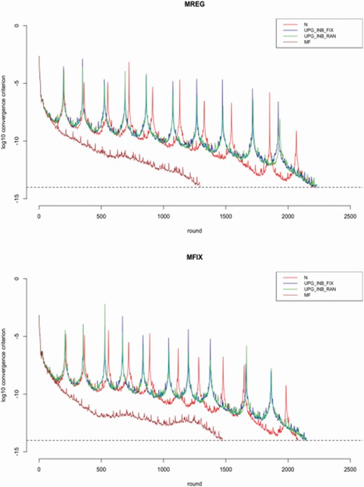
Rounds until convergence for each scenario. The first box corresponds to MREG, while the second corresponds to MFIX. The dashed line denotes the logarithm with base 10 of the convergence criterion. MREG refers to a model without parents’ origin fitted as a fixed effect. MFIX refers to a model with parents’ origin fitted as a fixed effect.
Table 3 presents the estimated accuracy of the predictions for each scenario and each trait. Values near one indicate that the EBV are accurately estimated. The concordance between and depends on the model and the trait. For MREG, both and were different for CYC1, FE1, and FE2. When MF were used, the two measures of prediction accuracy became similar for FE1 and FE2. On the other hand, for MFIX, the predictive ability and LR method performed similarly, except for CYC1. The largest difference between and was 0.34 for MREG and 0.15 for MFIX. In general, differences among models were not large. The highest accuracies were obtained using MF in MREG, whereas, for MFIX, the greatest accuracies were obtained with UPG with estimated inbreeding. Within models, no differences were observed among scenarios for some traits (e.g., CYC1).
Accuracy of predictions for each combination of model scenario1 and each trait estimated with both and
| WGT | CYC1 | FE1 | CYC2 | FE2 | ||||||
|---|---|---|---|---|---|---|---|---|---|---|
| MREGN | 0.72 | 0.72 | 0.50 | 0.59 | 0.39 | 0.63 | 0.59 | 0.57 | 0.29 | 0.63 |
| MREGUPG_INB | 0.73 | 0.71 | 0.50 | 0.58 | 0.40 | 0.59 | 0.58 | 0.61 | 0.32 | 0.52 |
| MREGUPG_INB_RAN | 0.73 | 0.71 | 0.50 | 0.58 | 0.40 | 0.59 | 0.58 | 0.61 | 0.32 | 0.52 |
| MREGMF | 0.73 | 0.70 | 0.62 | 0.83 | 0.69 | 0.69 | 0.67 | 0.80 | 0.58 | 0.61 |
| MFIXN | 0.79 | 0.74 | 0.59 | 0.69 | 0.63 | 0.65 | 0.58 | 0.61 | 0.63 | 0.64 |
| MFIXUPG_INB_RAN | 0.82 | 0.79 | 0.59 | 0.73 | 0.63 | 0.67 | 0.57 | 0.65 | 0.63 | 0.66 |
| MFIXUPG_RAN | 0.82 | 0.79 | 0.59 | 0.73 | 0.63 | 0.67 | 0.57 | 0.65 | 0.63 | 0.66 |
| MFIXMF | 0.71 | 0.69 | 0.58 | 0.74 | 0.59 | 0.62 | 0.61 | 0.71 | 0.52 | 0.57 |
1Models are defined as MREG and MFIX, while scenarios are denoted with the subscript in each line (N, UPG, UPG_INB, UPG_INB_RAN, and MF).
Table 4 presents the estimated dispersion of the predictions from the LR method for each scenario and each trait. Values near one indicate that there is no over/under dispersion in the GEBV. For MREG, the GEBV for CYC1, FE1, and FE2 were inflated except when MF were implemented in the evaluation. No considerable inflation was observed for any situation in MFIX. Within the range of 0.90 to 1.10, we considered the inflation/deflation as acceptable. Overall, for MREG, the best performance was achieved when MF were included in the model, whereas the worst performance was with UPG and estimated inbreeding. For MFIX, the best performance was obtained without modeling the genetic groups.
Dispersion of predictions for each scenario1 and each trait
| WGT | CYC1 | FE1 | CYC2 | FE2 | |
|---|---|---|---|---|---|
| MREGN | 1.01 | 0.87 | 0.71 | 1.05 | 0.62 |
| MREGUPG_INB | 0.98 | 0.85 | 0.69 | 1.00 | 0.62 |
| MREGUPG_INB_RAN | 0.98 | 0.85 | 0.69 | 1.00 | 0.62 |
| MREGMF | 1.05 | 0.90 | 1.11 | 0.96 | 1.01 |
| MFIXN | 0.99 | 0.99 | 1.01 | 1.00 | 0.98 |
| MFIXUPG_INB | 0.98 | 0.96 | 0.98 | 0.95 | 0.95 |
| MFIXUPG_INB_RAN | 0.98 | 0.96 | 0.98 | 0.95 | 0.95 |
| MFIXMF | 0.99 | 0.93 | 0.97 | 0.92 | 0.91 |
1Models are defined as MREG and MFIX, while scenarios are denoted with the subscript in each line (N, UPG, UPG_INB, UPG_INB_RAN, and MF).
Table 5 presents the estimated bias of the predictions for each scenario and each trait, expressed proportionally to the genetic standard deviation of each trait. Values near zero indicate that the EBV are unbiased. For all the traits, the bias was reduced when a fixed effect representing the origin of parents was fitted to the data (i.e., MFIX). The absolute value of the bias for MREG ranged from 0.10 to 0.69 standard deviations, whereas for MFIX the absolute bias ranged from 0.01 to 0.18. Except for WGT, the least biased predictions for MREG were obtained when MF were included in the model. For MFIX, the least biased predictions were obtained without including genetic groups and with UPG with estimated inbreeding.
Bias of predictions for each scenario1 expressed in terms of the genetic standard deviation of each trait
| WGT | CYC1 | FE1 | CYC2 | FE2 | |
|---|---|---|---|---|---|
| MREGN | −0.10 | 0.30 | −0.69 | −0.24 | −0.59 |
| MREGUPG_INB | −0.07 | 0.27 | −0.61 | −0.21 | −0.51 |
| MREGUPG_INB_RAN | −0.07 | 0.27 | −0.61 | −0.21 | −0.51 |
| MREGMF | 0.19 | 0.17 | 0.52 | −0.02 | 0.40 |
| MFIXN | −0.01 | 0.03 | 0.01 | −0.02 | 0.02 |
| MFIXUPG_INB | −0.01 | 0.03 | 0.01 | −0.02 | 0.02 |
| MFIXUPG_INB_RAN | −0.01 | 0.03 | 0.01 | −0.02 | 0.02 |
| MFIXMF | 0.03 | 0.09 | 0.18 | −0.09 | 0.18 |
1Models are defined as MREG and MFIX, while scenarios are denoted with the subscript in each line (N, UPG, UPG_INB, UPG_INB_RAN, and MF).
Discussion
The best way to model the inclusion of a group of external individuals in the evaluation was via the addition of an extra fixed effect representing the origin of the parents of the individuals, that is, local and external. Although the impact in accuracy is small, the GEBV with MFIX were almost unbiased and without inflation/deflation. For all traits, the phenotypic means in C2 were different among groups. Thus, dismissing α leads to a model misspecification (Rencher and Schaalje, 2008, Section 7.9).
Although the data and results show that α should be included in the model, this new parameter is hard to interpret in this situation because all focal individuals were born in the local environment. Hence, it is likely that α may be modeling a genetic effect absent in MREG. In fact, fitting α as a fixed effect accounts for nongenetic and genetic differences between parents of local and external individuals, whereas UPG account only for the genetic differences. If only UPG are considered, the nongenetic differences are not going to be modeled. The consideration of α as a fixed effect instead of random was to avoid the reestimation of variance components and to keep model simplicity. Although the reestimation of variance components may not be a limitation for smaller datasets, it can be time-consuming when the number of genotyped animals and traits is large. This can lead to a limitation in the interval between successive genetic evaluations and, therefore, become a problem for companies.
In this study, two estimators for the accuracy were used. Predictive ability is widely used but depends on model specification and will tend to be higher with over-parametrized models. That is, when increasing the number of fixed effects, the predictive ability will tend to overestimate the accuracy of GEBV. As an extreme example, with a saturated model (one fixed effect per animal) will be equal to 1, whereas will be equal to zero. It can be observed in Table 3 that greatly varied when the extra fixed effect was added into the model, whereas showed smaller changes. The average difference between and for MREG was 0.10, whereas for MFIX it was 0.06. It can be observed that for some traits greatly varied from MREG to MFIX. For example, it varied from 0.39 to 0.63 for FE1 when no genetic groups were modeled. On the other hand, varied from 0.63 to 0.65 for the same scenario. The addition of a simple fixed effect may not justify the increase in accuracy when using . Additionally, as an example, the correlation between GEBV for FE1 estimated with MREGN and MFIXN was 0.92. Clearly, this shows that the accuracy is wrongly estimated by in MREG. For the same scenario in Table 5, it can be observed that the bias greatly decreased from −0.69 to 0.01 standard deviations. Thus, it can be deduced that is more influenced by the model specification than . In other words, when a fixed effect like α is omitted from the model, the estimates of the accuracy with predictive ability greatly vary. Therefore, the use of for further evaluations is recommended since it depends less on the modeling of fixed effects. Different ways to compute exist depending on how the denominator is constructed (Legarra and Reverter, 2018; Macedo et al., 2020). However, the differences may be small and all the forms are proportional.
The accuracy of predictions with MF estimated with both and decreased significantly from MREG to MFIX. Also, predictions with MF in MFIX were more biased than with other methods. These issues may be related with the scaling of the genetic variance due to MF. As mentioned in Materials and Methods, when using MF in ssGBLUP, the genetic variance and consequently the inverse of the relationship matrix are divided by k. The way of computing k implicitly assumes that all MF have the same amount of information in the population. When groups to define MF are very unbalanced, as, in the case of C1, this assumption may be incorrect. If the group of external birds was larger, there would possibly be no issues of reduced accuracy and biased predictions with the inclusion of MF. However, further research is needed to solve this issue when the groups used to define MF are unbalanced and no other group definition can be used to determine the number of MF. In agreement with previous studies (van Grevenhof et al., 2019), the use of MF resulted in better convergence properties than other methods because of a reduction in the condition number of the system.
Conclusions
The inclusion of animals from an external group into local genetic evaluations should be correctly modeled to obtain accurate, unbiased, and not under-/over-dispersed GEBV. This can be done by including an extra fixed effect in the model, by using UPG or MF. For most of the traits in this study, the best scenario includes an extra fixed effect and with an extra adjustment as UPG with estimated inbreeding or MF. When the groups to define the MF greatly differ in the number of animals, predictions can be biased. In such a situation, it may be better to use UPG. Further research on this topic is needed. In this study, UPG without estimated inbreeding did not converge. Thus, taking into account estimated inbreeding for UPG is recommended. The use of MF reduced the condition number of the system, resulting in faster convergence for both models; however, this result cannot be generalized to other models and datasets. The estimation of accuracy using the LR method is less sensitive to the fixed effects of the model than predictive ability, therefore, being a proper method to the estimate accuracy of GEBV, independently of model specification.
Abbreviations
- APY
Algorithm for Proven and Young
- BLUP
best linear unbiased prediction
- CYC1
carcass yield component 1
- CYC2
carcass yield component 2
- EBV
estimated breeding values
- FE1
feed efficiency 1
- FE2
feed efficiency 2
- GEBV
genomic estimated breeding values
- MF
metafounders
- MREGMF/MFIXMF
models evaluated with MF
- MREGN/MFIXN
models evaluated without the inclusion of UPG
- MREGUPG/MFIXUPG
models evaluated with UPG without estimated inbreeding for UPG
- MREGUPG_INB/MFIXUPG_INB
models evaluated with UPG and estimated inbreeding for UPG
- MREGUPG_INB_RAN/MFIXUPG_INB_RAN
models evaluated with random UPG and estimated inbreeding for UPG
- ssGBLUP
single-step GBLUP
- UPG
unknown parent groups
- WGT
weight
Acknowledgment
This study was supported by Cobb-Vantress Inc. (Siloam Springs, AR).
Conflict of interest statement
The authors declare that they do not have any conflict of interest.
Data Availability
The data belong to Cobb-Vantress and, therefore, cannot be shared.
