


Abstract
The objectives of this study are to construct the high definition phenotype (HDP), a novel time-series data structure composed of both primary and derived parameters, using heterogeneous clinical sources and to determine whether different predictive models can utilize the HDP in the neonatal intensive care unit (NICU) to improve neonatal mortality prediction in clinical settings.
A total of 49 primary data parameters were collected from July 2018 to May 2020 from eight level-III NICUs. From a total of 1546 patients, 757 patients were found to contain sufficient fixed, intermittent, and continuous data to create HDPs. Two different predictive models utilizing the HDP, one a logistic regression model (LRM) and the other a deep learning long–short-term memory (LSTM) model, were constructed to predict neonatal mortality at multiple time points during the patient hospitalization. The results were compared with previous illness severity scores, including SNAPPE, SNAPPE-II, CRIB, and CRIB-II.
A HDP matrix, including 12 221 536 minutes of patient stay in NICU, was constructed. The LRM model and the LSTM model performed better than existing neonatal illness severity scores in predicting mortality using the area under the receiver operating characteristic curve (AUC) metric. An ablation study showed that utilizing continuous parameters alone results in an AUC score of >80% for both LRM and LSTM, but combining fixed, intermittent, and continuous parameters in the HDP results in scores >85%. The probability of mortality predictive score has recall and precision of 0.88 and 0.77 for the LRM and 0.97 and 0.85 for the LSTM.
The HDP data structure supports multiple analytic techniques, including the statistical LRM approach and the machine learning LSTM approach used in this study. LRM and LSTM predictive models of neonatal mortality utilizing the HDP performed better than existing neonatal illness severity scores. Further research is necessary to create HDP–based clinical decision tools to detect the early onset of neonatal morbidities.
INTRODUCTION
The most vulnerable patients with life-threatening conditions who require comprehensive care and constant monitoring are admitted to hospital intensive care units (ICUs). Depending on the patient’s age and medical condition, the patient could be admitted to specialized ICUs such as a neonatal intensive care unit (NICU),1 a pediatric intensive care unit,2 or a neurointensive care unit.3 The mortality in an adult ICU can range from 10% to 29%, depending on age, illness severity, and morbidities.4 The average mortality rate in very low birth weight (VLBW) and critically sick neonates in NICUs can be even higher, ranging from 6.5% to 46%.5–9
Several risk assessment scores have been developed to calculate hospital mortality rates, supporting decision-making by providing early predictions about the onset of severe acute disease states in high-risk patients.10 They sometimes help clinicians prioritize patient care in extreme cases, thereby helping to manage ICU resources. This can decrease the financial burden on the family and health system as it can improve the clinical outcomes of the health care unit overall.11,12
In the past two decades, various neonatal risk assessment scores have incorporated physiological vital signs, along with antenatal, perinatal, and laboratory data.13,14 Some studies have focused on patterns of variations in body temperature (BT) and cardiorespiratory signals such as heart rate (HR), respiratory rate (RR), peripheral oxygen saturation (SpO2), and blood pressure (BP).15 Previous studies have found that variabilities in HR, such as the heart rate characteristic (HRC) or heart rate variability (HRV) and its cross-correlation with other vital signs (HR-SpO2), are early markers for sepsis, necrotizing enterocolitis (NEC), and bronchopulmonary dysplasia (BPD).16 Other studies have shown that hypotension and the number of apnea events can predict the severity of intraventricular hemorrhage (IVH), retinopathy of prematurity (ROP), and BPD.17 Various data-driven models such as PhysiScore,18 PISA,13 and PROMPT19 have used machine learning techniques to explore time series ICU data for generating risk assessment scores.
Enormous quantities of data are collected for each patient in an ICU, including time-series data updated every second (such as monitored physiological data), vital signs, diagnosis records, medication and nutrition data, laboratory reports, imaging results, medical staff notes, and more. This vast data production has resulted in the generation of some multimodal temporal databases that encapsulate the integrated big data of an ICU such as MIMIC I, II, and III.20,21
This study highlights the importance of understanding the enormous amounts of data in areas such as critical care and use that to improve patient outcomes. We capture time-series NICU data into an original structure referred to as the high definition phenotype (HDP). The data are categorized using a series of fixed, intermittent, and continuous data to form a HDP. This is used to create a prediction model for neonatal mortality. The developed model uses both the logistic regression model (LRM) and the long–short-term memory (LSTM) models and helps to validate the HDP’s functionality in supporting time series predictive analyses. This provides real-time bedside probability of mortality utilizing different parameters across the length of stay in the NICU. We present case studies for death and discharge cases to illustrate how predictive models might be used as a decision-making tool in clinical settings.
METHODS
Clinical settings
This study was conducted at eight level III NICUs of a corporate hospital group across India. All the units have at least 15 beds and similar infrastructure and patient care facilities and are largely representative of other major level III NICUs in the country. None of the study NICUs support ECMO. There are various data sources in the NICU, like the electronic medical record (EMR), laboratory information management system (LIMS), and biomedical equipment such as patient monitors, ventilators, and blood gas machines. The Institutional Review Board of the study NICUs approved the collection of data from all these sources with a waiver of informed consent. All electronic health records were deidentified in accordance with the United States Health Insurance Portability and Accountability Act (HIPAA), and all the research was performed according to local institutional guidelines.
HDP data
The HDP divides data into two broad categories: primary and derived. Data are considered primary if its clinical interpretation is well defined, that is, birth weight, HR, temperature, SpO2, and urine output. Derived parameters are extracted from the primary data and represent additional information such as trends or variability. Both primary and derived parameters are further classified into three categories: fixed (F), intermittent (I), and continuous (C). The fixed parameters consist of values that do not change over the course of the patient’s hospitalization, such as some antenatal and perinatal data (eg, gestational age, birth weight, sex, etc.) The intermittent parameters contain clinical information collected periodically during the hospital stay, such as daily weight, BP (although BP monitoring using an arterial line is considered a continuous parameter since few study infants had invasive BP monitoring, BP was analyzed as an intermittent parameter), blood pH, lab values, and medication information. Continuous parameters are fine-grained consecutive data such as time-stamped vital signs collected from physiological monitors, for example, HR, RR, and SpO2. Some of these monitors used in NICUs (such as GE B40® patient monitor, GE Healthcare, and the SureSigns® VM6 patient monitor, Philips Medical Systems) can only provide data at a minute resolution. Based on the literature review, we utilized 49 commonly collected data parameters evaluated in previously identified studies (Supplementary Table S1) to instantiate the HDP.
As stated previously, derived parameters are abstracted from primary data and represent additional information. Examples of derived information include data regularity, stationarity, frequency components of primary data, or the cross-correlation between two parameters such as HR and SpO2. Various studies have utilized these derived parameters in building prediction models for the early onset of disease or mortality. Moorman and colleagues have used sample entropy in HRV as an early marker of disease such as neonatal sepsis.22,23 Other studies have used stationarity of time-series temperature data using augmented Dickey–Fuller statistics to predict infant mortality. The stationarity of time-series laboratory reports has been used to forecast viral respiratory illness in PICU.24 The central tendency and spread of HRV have been used amongst patients with severe sepsis and septic shock to predict discontinuance of vasopressor medications after ICU admission.25 Additionally, studies have utilized topic models in longitudinal EMR data to discover features used to predict disease severity in the ICU.26
The above studies have validated complex relationships between diverse physiological parameters and the onset of diseases, thus signifying the importance of both primary and derived data. This study similarly used a collection of acquired data and then augmented it with derived data to create the HDP of a patient. The HDP was fed into two different models, one based on a LRM and the other on a LSTM deep learning system to create prediction programs (Figure 1).
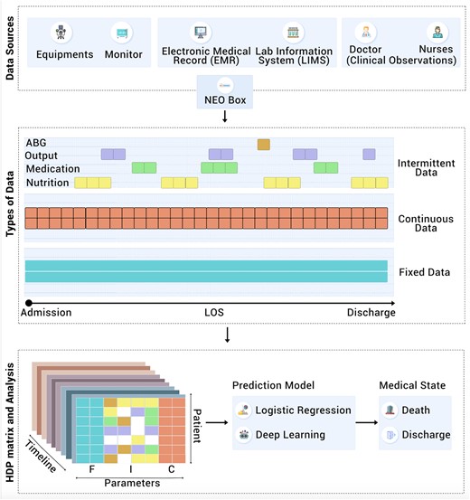
Architectural overview of data source, types of data, preparation of HDP data structure and its analysis (F: Fixed, I: Intermittent, C: Continuous parameters).
Deep learning models are successful in utilizing high-resolution time-series medical data in intensive care units.27 In this study, we chose an LSTM approach28 to deep learning because LSTMs have been used successfully to model complicated dependencies in time-series data.29 LSTMs have achieved state-of-the-art results in many different medical applications.30–32 They are well-suited to describe a medical dataset where the patient's clinical state is spread over several minutes, hours, and days. On the other hand, the statistical approach using the LRM is a recognized technique for analyzing large data sets and can be used to elucidate how certain features of the data set are associated with the outcomes. Studying both the LRM and the LSTM models helps validate the HDP’s functionality in supporting time-series predictive analyses.
Study design
Initial clinical data of 1546 patients were collected using a NEO data aggregator device that collects physiological data from medical devices like bedside monitors and ventilators in a vendor-agnostic manner.33 Patients in a study NICU from July 2018 to May 2020 who stayed in the NICU for >24 hours and were sick enough to have continuous parameters recorded were included in the study. All the congenital anomalies, readmission, discharge on request, left against medical advice, and transfer cases were excluded from the study, leaving a total of 757 cases (742 discharge and 15 deaths) for study analysis. The reported incidence of congenital anomalies is 1%–4%;34 the neonates with congenital anomalies represent a group with the risk of mortality. However, for this feasibility study, keeping in mind the sample size, the neonates with congenital anomalies were excluded.
Data preparation and processing
For this study, data were collected through the iNICU EMR platform35 which implements a neonatal data dictionary36 capturing the complete workflow of the NICU. The data collected in the NICU were segregated into fixed, intermittent, and continuous fields to build the HDP time-series data structure. Data visualization was performed by presenting every attribute against time to compare and observe the correlation between the variables (Figure 2).
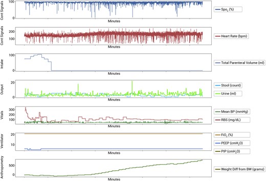
Data visualization of HDP parameters with respect to time.
To prepare the data set of the study for the predictive model, all the death and discharge cases were considered and balanced based on the length of the stay in NICU. Data contain a total of 757 cases (742 discharge and 15 deaths). To balance the dataset in the LSTM model, we analyzed all 15 death and 15 randomly selected discharge cases. The cases in both the group were matched for their length of stay. This ensured the equal number of minute wise HDP values were present for both the groups.
Data imputation was carried out for missing data for each fixed, intermittent, and continuous data types. Imputation and detailed data curation steps are discussed in Supplementary Method S1.
The data set was split into a training and testing set in a 70:30 ratio. The results discussed in this study are from running the LRM and LSTM predictive models on the testing set. None of the cases in the testing set were used to train either predictive model.
The computational analysis was carried out on two custom configurations. The first configuration consists of the Hadoop HD Insight cluster (Hadoop 3.2.1 on Azure cloud platform) with 200 Cores in Japan region with 12 nodes consisting of 1 master (2 nodes) and 10 worker nodes of D14 configuration each [v2, 16 cores, 112 GB random-access memory (RAM)]. The second configuration consists of the D-Series Azure Virtual machine, which features 2.3 GHz Intel XEON® E5-2673 v4 (Broadwell) processors. The virtual machine of the second configuration consists of 32 CPU cores and 128 GiB of RAM. The mapper, reducer, and the HDP–based machine learning algorithms were implemented using Python 3.5. The Python libraries used were pandas, numpy, psycopg2, sklearn, imblearn, seaborn, math, random, statsmodels, nolds, entropy, matplotlib, scipy, tensorflow, keras, prettytable, itertools, os, sys, linecache, pylab, and datetime.
HDP matrix preparation
Based on the 49 parameters selected for the study, 1546 patients had baseline data available. Out of these, 1188 patients had intermittent data, and 788 patients had continuous data during hospitalization. The reason for the difference in intermittent and continuous data were twofold (1) some patients were not connected with NEO devices for real-time data capturing, causing loss of continuous data and (2) nutrition and medication entries were not made for patients who were either discharged next day or sent back to mother as they were not ill enough to be kept in NICU. The intersection of patients containing all three fixed, intermittent, and continuous data was 757 patients. During the NICU stay, the patients are occasionally removed from devices for procedures, or the probes get disconnected due to routine movements. This results in missing data, which needs prior management. The distribution of data imputation for various fields is presented in Supplementary Table S7.
Development of the models
A leave-one-out cross-validation strategy37 was used in both LRM and LSTM models during the model development.
LRM model
Logistic regression with l2 regularization38 was used as the LRM. In order to compensate for the skewed distribution of samples (death vs discharge) in this study, we have used an oversampling technique called synthetic minority oversampling technique (SMOTE) to balance the training set.39 During the training phase analysis, the SMOTE boosting runs in conjunction with logistic regression (Figure 3).
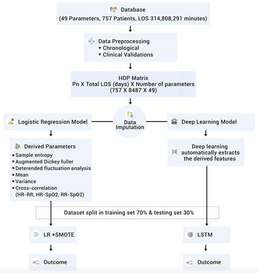
Detailed flow chart of data preparation, imputation and analysis, LOS: Length of Stay, Pn: Patient number LR: Logistic Regression, SMOTE: Synthetic Minority Oversampling Technique, LSTM: Long Short Term Memory.
LSTM model
In this study, a two-layer LSTM model28 was implemented, with the first layer being a bidirectional LSTM with 512 connections and the second layer with an LSTM with 256-dimensional cell state and no dropouts (detailed features are discussed in Supplementary Method S2).40 Both the layers use tanh activations for the cell states of the LSTM, while the output layer has a sigmoid activation, as is typical for binary classification problems (death vs discharge). Though, ReLU activations have been very successful in deep feed-forward networks (eg, CNNs); however, for LSTMs, ReLU–based activation requires careful initialization in order to avoid exploding gradients.41 Therefore, in our LSTM–based model, tanh activation has been used. The tanh activation is also used successfully with LSTM model in the previous studies on ICU data (MIMIC III).40 The LSTM validation was done with a random split of data into 10-fold cross-validation.
Model performance testing
The HDP data were processed with LRM and LSTM–based techniques at different time points of the patient stay (1 hour, 6 hours, 12 hours, 48 hours, 1 week, 2 weeks, 3 weeks, 4 weeks, and the total length of stay) to generate a prediction model. The mortality prediction performance of the LRM and LSTM models were compared with other severity scores such as the clinical risk index for babies (CRIB), CRIB-II, the score for neonatal acute physiology II (SNAP-II), and the SNAP-perinatal extensions II (SNAPPE-II) used in NICU settings (based on parameters presented in Table 1). Model performance was assessed based on the area under the receiver operating characteristic curve (AUC-ROC), and the sensitivity, specificity, and accuracy were also evaluated.
List of parameters of CRIB, CRIB-II, SNAP-II, SNAPPE-II, and LRM and LSTM scores
| CRIB (n = 244) | CRIB-II (n = 1166) | SNAP-II (n = 1546) | SNAPPE-II (n = 1546) | LRM (n = 1546) | LSTM (n = 1546) | |
|---|---|---|---|---|---|---|
| Number of parameters | 6 | 4 | 6 | 9 | 49 | 49 |
| Qualifying criteria | ||||||
| Birth weight (g) | <1500 | All | All | All | All | All |
| Gestation (weeks) | ≤32 | ≤32 | All | All | All | All |
| Valid until hour | 12 | 1 | 12 | 12 | LOS | LOS |
| Parameters | ||||||
| Birth weight | ✓ | ✓ | ✓ | ✓ | ✓ | |
| Gestation | ✓ | ✓ | ✓ | ✓ | ✓ | |
| Maximum base excess | ✓ | ✓ | ||||
| Congenital malformation | ✓ | |||||
| FiO2 | ✓ | ✓ | ✓ | |||
| Gender | ✓ | ✓ | ✓ | |||
| Temp at admission | ✓ | |||||
| Mean BP | ✓ | ✓ | ✓ | ✓ | ||
| Lowest temp | ✓ | ✓ | ||||
| pH | ✓ | ✓ | ✓ | ✓ | ||
| PO2/FiO2 ratio | ✓ | ✓ | ||||
| Multiple seizures | ✓ | ✓ | ||||
| Urine | ✓ | ✓ | ✓ | ✓ | ||
| APGAR | ✓ | ✓ | ✓ | |||
| Systolic BP | ✓ | ✓ | ||||
| Diastolic BP | ✓ | ✓ | ||||
| Body weight | ✓ | ✓ | ||||
| Temp | ✓ | ✓ | ||||
| Heart rate | ✓ | ✓ | ||||
| Respiratory rate | ✓ | ✓ | ||||
| In/out born | ✓ | ✓ | ||||
| Mode of delivery | ✓ | ✓ | ||||
| Baby type (single/multiple) | ✓ | ✓ | ||||
| Conception type | ✓ | ✓ | ||||
| Random blood sugar | ✓ | ✓ | ||||
| Length | ✓ | ✓ | ||||
| Birth head circumference | ✓ | ✓ | ||||
| Mother's age | ✓ | ✓ | ||||
| Medication type | ✓ | ✓ | ||||
| Medication dose | ✓ | ✓ | ||||
| Nutrition | ✓ | ✓ | ||||
| Cross-correlation HR-SpO2 | ✓ | |||||
| Cross-correlation HR-RR | ✓ | |||||
| Cross-correlation RR-SpO2 | ✓ | |||||
| Sample entropy | ✓ | |||||
| Variance | ✓ | |||||
| Detrended fluctuation analysis | ✓ | |||||
| Mean | ✓ | |||||
| Augmented Dickey–Fuller | ✓ |
BP, blood pressure; CRIB: clinical risk index for babies; HR: heart rate; LRM: logistic regression model; LSTM: long–short-term memory; LOS: length of stay; RR: respiratory rate; SpO2: peripheral oxygen saturation SNAP-II: score for neonatal acute physiology II; SNAPPE-II: SNAP-perinatal extensions II.
Data deidentification
Data collection was based on Fast Healthcare Interoperability Resources (FHIR) protocols. Data collected for the study were deidentified, and the patient database adheres to HIPAA standards. Patients’ names, unique id, and other identifiable demographic information, including date of birth and date of admission were removed before analysis.
RESULTS
Baseline data
The baseline dataset included 1546 patients (877 males and 669 females) comprising 25 death and 1521 discharged cases (Table 2). 80% of non–surviving cases have gestation <32 weeks and birth weight <1500 g. The study shows several other parameters, including gestational age, birth weight, 1-minute APGAR, 5-minute APGAR, respiratory distress, and sepsis, vary significantly between the discharged vs death cases. Two-sided Welch’s test is used for two populations (death and discharge) having unequal sample distribution variance.
Baseline characteristics of the population
| Parameters | Death (n = 25) | Discharge (n = 1521) | P values |
|---|---|---|---|
| Gestationa | 29.7 (4.7) | 34.9(3.1) | <.001 |
| Mother’s agea | 31.9 (3.9) | 32.1 (5.5) | .838 |
| Conception type (IVF)b | 14 (56.0%) | 407 (26.7%) | .001 |
| Antenatal steroidsb | 12 (48.0%) | 443 (29.1%) | .04 |
| Mode of delivery (LSCS)b | 17 (68.0%) | 910 (59.8%) | .408 |
| Out bornb | 4 (16.0%) | 315 (20.7%) | .564 |
| Baby type (multiple)b | 18 (72.0%) | 712 (46.81%) | <.001 |
| Gender (male)b | 14 (56.0%) | 863 (56.74%) | .941 |
| APGARa | |||
| One minute | 6.2 (1.2) | 7.8 (0.8) | <.001 |
| Five minutes | 7.4 (0.9) | 8.8 (0.5) | <.001 |
| Ten minutes | 8.5 (0.8) | 9.3 (0.6) | .057 |
| Birth weighta | 1342.2 (844.3) | 2338.6 (705.8) | <.001 |
| Birth head circumferencea | 28.5 (4.8) | 32.4 (2.8) | .103 |
| Jaundice with phototherapy | 11 (44.0%) | 648 (42.6%) | .889 |
| Sepsis | 16 (64.0%) | 168 (11.05%) | <.001 |
| Respiratory distress syndrome | 19 (76.0%) | 62 (4.1%) | <.001 |
APGAR: appearance, pulse, grimace, activity, and respiration; IVF: in vitro fertilization; LOS: length of stay; LSCS: lower segment cesarean section.
Mean (standard deviation).
Count (percentage within that class).
Ablation experiments
The ablation experiments for fixed, intermittent, continuous parameters, and their combinations to estimate the weights of these parameters for the LRM and LSTM models are shown in Table 3. When considered alone, continuous parameters in both models have the best predictive performance (0.83 and 0.88 AUC, respectively). The combination of fixed, continuous, and intermittent parameters improved the AUC to 0.86 for LRM and 0.95 for LSTM (Table 3). It was observed that SpO2, a continuous parameter, has a significant contribution with the AUC-ROC score of 0.81 (Supplementary Table S8). Various combinations of pulse rate (PR), SpO2, and RR have more than 0.80 AUC scores (Supplementary Table S9). While in the case of intermittent parameters, urine output has a maximum contribution with the AUC score of 0.88 (Supplementary Table S10). These AUCs reported are from a validation dataset.
Ablation experiments for the contribution of fixed, intermittent, and continuous during mortality prediction
| LSTM | LRM | |||||
|---|---|---|---|---|---|---|
| Subcomponents | AUC-ROCa | F1-score | AUPRC | AUC-ROCa | F1-score | AUPRC |
| Fixed | 0.47 ± 0.11 | 0.51 | 0.52 | 0.68 ± 0.04 | 0.62 | 0.46 |
| Intermittent | 0.87 ± 0.13 | 0.72 | 0.68 | 0.77 ± 0.05 | 0.70 | 0.49 |
| Continuous | 0.88 ± 0.13 | 0.77 | 0.71 | 0.83 ± 0.04 | 0.79 | 0.68 |
| Fixed + intermittent | 0.75 ± 0.19 | 0.66 | 0.60 | 0.75 ± 0.04 | 0.71 | 0.57 |
| Fixed + continuous | 0.69 ± 0.51 | 0.69 | 0.67 | 0.80 ± 0.03 | 0.77 | 0.65 |
| Intermittent + continuous | 0.91 ± 0.05 | 0.83 | 0.79 | 0.81 ± 0.03 | 0.78 | 0.75 |
| Fixed + intermittent + continuous | 0.95 ± 0.12 | 0.88 | 0.90 | 0.86 ± 0.04 | 0.80 | 0.79 |
AUC-ROC: area under the receiver operating characteristic curve; LRM: logistic regression model; LSTM: long–short-term memory.
AUC-ROC ± confidence intervals (95%).
Model performance
The performance of the model to predict mortality was assessed at different time periods: 1 hour, 6 hours, 12 hours, 48 hours, 1 week, 2 weeks, 3 weeks, and 4 weeks. The best performance of LRM was achieved at the 4th week, while the best performance of the LSTM is at the 48th hour (Table 4). The cutpoint used for computing the different evaluation metrics was the default value of 0.5, typically used with binary classifiers like logistic regression. The ROC curve or the precision-recall curve can be further analyzed to pick an appropriate operating point (or cutoff threshold), as is typically done before deployment. The emphasis of this experiment was to demonstrate the models’ general capability to process the input data and predict mortality, as opposed to achieve the best performance on this specific dataset. To evaluate the performance of the developed model, the most fragile and at risk infants group was used to predict the mortality (Supplementary Method S3).
Summary of LRM and LSTM mortality detection performance at different time points
| Time of Prediction | AUC-ROC (LRM) | PPV (LRM) | NPV (LRM) | AUC-ROC (LSTM) | PPV (LSTM) | NPV (LSTM) |
|---|---|---|---|---|---|---|
| 1 hour | 0.59 ± 0.02 | 0.75 ± 0.09 | 0.62 ± 0.08 | 0.88 ± 0.02 | .0.96 ± 0.02 | 0.71 ± 0.06 |
| 6 hours | 0.72 ± 0.03 | 0.85 ± 0.03 | 0.75 ± 0.02 | 0.89 ± 0.03 | 0.73 ± 0.05 | 0.81 ± 0.03 |
| 12 hours | 0.75 ± 0.01 | 0.85 ± 0.05 | 0.80 ± 0.03 | 0.93 ± 0.01 | 0.92 ± 0.02 | 0.84 ± 0.02 |
| 48 hours | 0.73 ± 0.03 | 0.82 ± 0.04 | 0.85 ± 0.04 | 0.95 ± 0.01 | 0.97 ± 0.01 | 0.85 ± 0.01 |
| 1 week | 0.71 ± 0.01 | 0.79 ± 0.03 | 0.70 ± 0.02 | 0.91 ± 0.02 | 0.85 ± 0.04 | 0.92 ± 0.02 |
| 2 weeks | 0.79 ± 0.02 | 0.86 ± 0.01 | 0.75 ± 0.04 | 0.90 ± 0.03 | 0.79 ± 0.06 | 0.90 ± 0.02 |
| 3 weeks | 0.72 ± 0.02 | 0.80 ± 0.07 | 0.71 ± 0.03 | 0.91 ± 0.01 | 0.82 ± 0.02 | 0.93 ± 0.01 |
| 4 weeks | 0.82 ± 0.01 | 0.88 ± 0.02 | 0.77 ± 0.06 | 0.90 ± 0.02 | 0.88 ± 0.03 | 0.79 ± 0.03 |
| Total length of stay | 0.81 ± 0.02 | 0.89 ± 0.02 | 0.80 ± 0.02 | 0.96 ± 0.01 | 0.80 ± 0.03 | 1.0 ± 0.01 |
AUC-ROC: area under the curve receiver operating characteristic curve; CI: class interval; LRM: logistic regression model; LSTM: long–short-term memory; NPV: negative predictive value; PPV: positive predictive value.
Comparison with existing models
The CRIB, CRIB-II, SNAP-II, SNAPPE-II, LRM, and LSTM scores were compared for predicting death and discharge at the respective time points where each score is applicable. The performance of the LSTM model was compared with other severity scores using the validation dataset. A comparison of sensitivity, specificity, and accuracy is shown for each model in Figure 4. ROC curves are represented in Figure 5 and Supplementary Table S6.
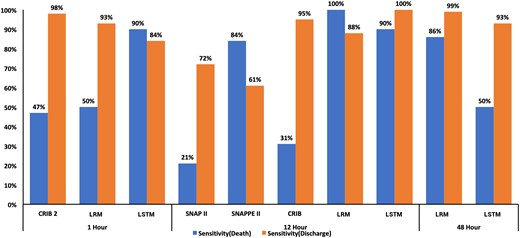
Comparison of CRIB (at 12 hours), CRIB-II (at 1 hour), SNAP-II (at 12 hours), SNAPPE-II (at 12 hours), and probability (at 48 hours) for predicting death and discharge.
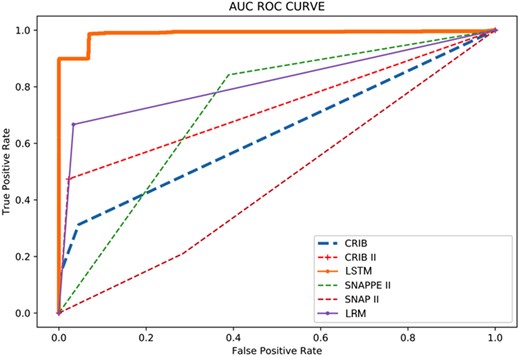
Receiver Operating Characteristic Curve of the CRIB, CRIB-II, SNAP-II SNAPPE-II, LRM and LSTM.
Case studies
This section shows two case studies, one for death and another for a discharged patient, to demonstrate how the prediction model varies over time during the hospital course. Using the LSTM prediction model, we have developed a real-time probability of death across the entire length of stay in the NICU. We used a probability threshold of 0.5 to predict death based on the standard convention followed for a balanced dataset.42 The probability variation at any given time point based on the underlying health condition is represented as red and green dots. Any probability above 0.5 predicts death, and probabilities under 0.5 predict survival to discharge (Figure 6). The cut-off point (of 0.5) could be adjusted by analyzing the ROC curve for higher accuracy or precision required at specific NICU deployment.
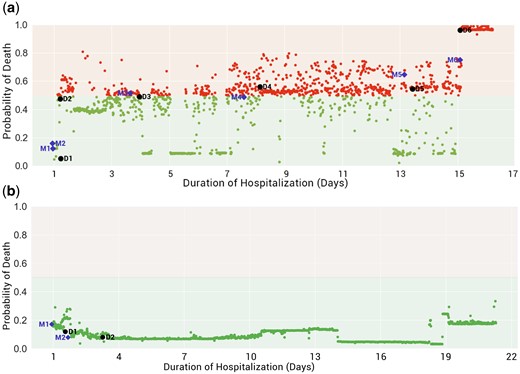
(a) Death case, (b) Discharge case (purple diamond represents the prediction of severe risk by the model, the black circle represents the severity suspected by the doctor), Mn: Anomaly detected by model, Dn: Time of assessment by the doctor.
The two case studies illustrate the possibility of how real-time prediction might be used at the bedside. Although the models in this study are trained specifically to predict mortality, one perspective is that a higher probability of death directly implies a higher severity of illness. Therefore, a real-time mortality predictor is functionally similar to a real-time severity of illness score.
Even though the current LSTM model is not explicitly trained for specific morbidities or their course of treatments, its prediction seems well synchronized with assessments and events in a patient stay during NICU. Interestingly, physiological deviations detected by the models (marked as Mn in Figure 6) predict and correlate with clinical morbid conditions observed by the doctor (marked as Dn in Figure 6).
In the following tables describing the case studies, time of assessment/clinical detection of the event means the time at which the doctor has observed an anomaly in the patient's condition. The assessment itself is the name of a predefined ICD9 medical state picked up by the doctor clinically. The deviation detected by the model is defined as the absolute percentage change in the value of probability between two consecutive time points. In this current feasibility study, a threshold of 10% and a patience of 4 is used. The patience value signifies that the difference from the last value is maintained for 4 consecutive 15-minute intervals. The deviation time represents the time when the model detects an anomaly in the patient condition.
The convergence of the probability of death and discharge of <32 and >32 gestational age is represented in Supplementary Figure S1 with the normalized length of stay. The probability of mortality for each death patient is represented in Supplementary Figure S2.
Death case
In Figure 6 (a) and Table 5, we illustrate an example of changes in the clinical state of a deceased patient and the consequent real-time prediction of outcome (mortality) during the hospitalization. The main clinical events are described below (detail in Supplementary Method S3):
List of events detected by the doctor and the LSTM, LRM model, and interventions carried out for death case
| DOL (days) | Time of assessment/clinical detection of event | Name of event | Action taken/interventions | When the model has detected the deviation (time) | (LSTM, LRM) probability at clinical assessment | (LSTM, LRM) probability at deviation |
|---|---|---|---|---|---|---|
| 1 | At birth | RDS (1st episode) | NIMV | At admission | (0.044, 0.001) | (0.044, 0.001) |
| 1 | 3 hours | Apnea | NIMV, caffeine | At admission | (0.464, 0.011) | (0.044, 0.001) |
| 1 | 4 hours | Jaundice | Phototherapy | 17 hours | (0.50, 0.001) | (0.41, 0.144) |
| 6 | 96 hours | Jaundice (2nd episode) | Phototherapy | 82 hours | (0.47, 0.002) | (0.52, 0.002) |
| 8 | 192 hours | No pulses in lower limbs | ECHO for COA, prostaglandin | 147 hours | (0.57, 0.014) | (0.50, 0.014) |
| 12 | 306 hours | RDS (2nd episode) | CPAP | 299 hours | (0.53, 0.012) | (0.68, 0.002 |
| 13 | 310 hours | Sepsis | Amikacin, Meropenem | 299 hours | (0.54, 0.011) | (0.68, 0.002) |
| 14 | 353 hours | Worsen RDS | HFO | 341 hours | (0.94, 0.02) | (0.74, 0.017) |
Note: Time of assessment: time at which the doctor has observed an anomaly in the patient condition.
The deviation: time when the model/device detects an anomaly in the patient condition.
COA: coarctation of aorta; ECHO: echocardiogram; HFO: high frequency oscillator; LRM: logistic regression model; LSTM: long–short-term memory; NIMV: non–invasive mechanical ventilation; RDS: respiratory distress syndrome.
The patient was admitted with respiratory distress and was put on non–invasive mechanical ventilation (D1). The model detected a deviation at the same time represented as M1.
At day of life (DOL) 1, after 3 hours of admission, the doctor detected apnea (D2), predicted by the model at the time of admission (M2).
At DOL 4, the patient developed jaundice (D3) and was treated with phototherapy, predicted by the model (M3).
At DOL 8, the clinician observed absent pulses in the lower limbs of the patient and diagnosed the patient with coarctation of the aorta (COA) (D4).
At DOL 13, the probability of mortality was ∼54% as the model detected deviation (M5) ∼68%. Later the same day, the patient was suspected of having sepsis (D5) and was started on antibiotics.
At DOL 15, the probability of mortality increased to ∼74%, which was captured as deviation (M6), whereas the probability of mortality at a later time coincident with a physician assessment worsened to ∼90% (D6).
The patient died on DOL 19.
Discharge case
In Figure 6 (b) and Table 6, we illustrate an example of changes in the clinical state of a discharged patient and the consequent real-time outcome predictions (detailed clinical events are discussed in Supplementary Method S3):
List of events detected by the doctor and the (LSTM, LRM) model and interventions carried out for discharge case
| DOL (days) | Time of assessment/clinical detection of event | Name of event | Action taken/interventions | When the model has detected the deviation (time) | (LSTM, LRM) probability at clinical assessment | (LSTM, LRM) probability at deviation |
|---|---|---|---|---|---|---|
| 1 | 3 hours | RDS | CPAP | 1 hour | (0.13, 0.013) | (0.18, 0.014) |
| 1 | 3 hours | Apnea | CPAP to NIMV after 1 hour, piperacillin tazobactam, inj. amikacin, inj. caffeine (loading) | 1 hour | (0.13, 0.013) | (0.18, 0.014) |
| 2 | 51 hours | Jaundice | Phototherapy | 18 hours | (0.10, 0.035) | (0.12, 0.098) |
Note: Time of assessment: time at which the doctor has observed an anomaly in the patient condition.
The deviation: time when the model/device detects an anomaly in the patient condition.
CPAP: continuous positive air pressure; Inj.: injection; LRM: logistic regression model; LSTM: long–short-term memory; NIMV: non–invasive mechanical ventilation; RDS: respiratory distress syndrome.
The patient was admitted with respiratory distress syndrome (RDS). The model detected a deviation (M1) approximately an hour prior to clinician documentation of RDS at the third hour of life (D1).
The model was able to detect a deviation at 18 hours (D2), while the patient was noted to have jaundice at the age of 51 hours (M2).
The patients’ condition remained stable and was discharged on DOL24.
DISCUSSION
In this study, we have developed and validated the HDP time-series data model and constructed two bedside mortality prediction models based on the HDP. The mortality prediction models in this current study utilize statistical and deep learning approaches to illustrate the broad range of analyses that the HDP supports. There is no theoretical constraint, however, on the type of analytic approaches that can utilize the HDP, and other predictive techniques may be explored in future studies. Frequently used traditional scores such as the CRIB, CRIB-II, SNAP-II, and SNAPPE-II use limited information from the NICU (often first 24 hours following admission).43–45
Recent studies have reported prediction models based on time series data18,46,47 can detect the change in physiological parameters due to acute deterioration of health conditions before clinical suspicion. For instance, the Pediatric Risk of Mortality Prediction Tool (PROMPT), a real-time prediction score used in PICU, identifies the deteriorating health of patients.19 Similarly, the DeepSOFA framework predicts illness severity in ICU settings by leveraging deep learning with Sequential Organ Failure Assessment (SOFA). The DeepSOFA framework utilizes an individual’s physiological patterns and specific respiratory, cardiovascular, and hematology data from electronic health record data to calculate hourly predicted SOFA score.48 These studies show a continuous improvement in risk assessment scores with machine learning, artificial intelligence techniques, and data archiving hardware, facilitating the discovery of data-driven characteristics and patterns of diseases.49–51 The physiological data are continuously influenced by clinical interventions such as medication, oxygen supplementation given to the patient to maintain the steady-state.52
In this study, we have chosen to analyze 49 common parameters (fixed, intermittent, and continuous) recorded during the neonatal period based on our prestudy literature review. We recognize that other parameters may be potentially important variables, which can be considered in future studies. Our study builds upon this knowledge to leverage integrated ICU data built by combining real-time physiological data, laboratory results, and an EMR integrated platform. The iNICU35 EMR plugin fetches the clinical data from different EHR systems like Epic, Cerner, and Allscripts.53 It uses RedoxEngine54 to communicate with different EMR and communicate via HL7 message. Certain examples of these messages include admission-discharge details (ADT), observation record units (ORU-R01: Laboratory results data), and digital imaging and communications in medicine (DICOM)55 based data transfer to collate the data on a single interface. The solution is implemented as a plugin to EMR, which shows data on a web-interface in the tablet at the bed-side (Supplementary Figure S26). The entire record for a single patient is augmented with temporal information and derived data and referred to as the HDP. Incorporating continuously updated physiological data in the HDP allows the model to provide timely warnings of health deterioration. The LSTM–based model utilizes 15-minute data (configurable) chunks and predicts the probability of death or discharge or patient deterioration based on combined HDP data structure prior to clinician observation. However, the model does not provide the specific parameters or correlation between the parameters causing the deterioration. Moreover, this is a feasibility study where we have shown that this model provides a reasonable risk for the occurrence of an event. However, whether this early alert results in prompt action by the clinician and can subvert the occurrence or severity of an event needs to be evaluated in further clinical trials.
In the current study, the LSTM output was compared with existing severity scores along with traditionally used LRM. In the LSTM model, the complete data at per minute resolution are inserted as an input (consisting of independent variables). Even though the LSTM is performing better than other models, the current technology landscape of LSTM does not have explainability of prediction with respect to which all variables contribute significantly to the outcome variable. Even though the prediction by the LRM is slightly less compared to the LSTM model, it has the advantage of explainability regarding the contribution of the individual input variable. It was anticipated that as the system will be deployed at the bedside, it will be determined whether having both model outputs are useful.
This study has certain limitations. The study is based on retrospective data, and to validate the use in bedside clinical care, a prospective study needs to be done. In the current study, hospital readmission was an exclusion factor. The fixed factors, such as admission parameters in infants, who have readmissions, may not have the same predictive value for primary admissions. Since readmission may be considered a complication associated with morbidities or even mortality, future studies should include readmissions. A common and unavoidable property of real clinical data is missing data, which needs to be handled by imputation strategies. Various imputation strategies such as replacing missing values by (1) −999, (2) mean of remaining data, (3) previously known value of the parameter, and (4) building models from existing data to predict the missing values have been used in the literature. However, the type of imputation strategy used to handle missing data can affect the outcome of the deep learning models. Besides, the dataset included in the study includes only one year from eight sites, so the number of death cases were limited. Model performance can likely be further improved with a larger dataset, with validation testing on another external dataset. Whereas many current ICU physiological monitors can output waveform data, this study only utilizes per minute data for developing the prediction model due to device limitations at the current study sites. The current implementation of the model was done, utilizing only LRM and LSTM models. In the future, more machine learning algorithms could be utilized that may be even more suitable for managing time-series clinical data.
A vast amount of temporal patient information is stored in the HDP data structure at a regular interval. The current deep learning and regression models focus on hidden inter-relationships (represented in the derived data) in the HDP to predict an individual patient’s mortality. In the current study, the individual graphs for all death cases were studied, and it was observed that the line for each of the patients varies depending on the clinical severity and associated metabolic abnormalities. With a limited dataset, specific disease trends are difficult to the group due to a lack of data with respect to gestational age and birth weight. In future studies, we aim to identify disease-specific patterns for different gestational ages and birth weight categories and predict specific morbidities such as sepsis, NEC, and ROP by creating specific disease models. To achieve this, knowledge–based disease definition by capturing relevant features (collected from literature studies) could be curated. We aim to use higher fidelity (resolution) data in future studies, as more granular data can increase the sensitivity of the HDP–based model. Big data validation of prediction models in different settings could help lower the burden of caregivers by reliably identifying the most critical patients and supporting the development of intervention plans according to the available care resources.
Code availability
The code that underpins the prediction of mortality using the HDP dataset is openly available. The drive containing the code used to generate the descriptive statistics and tables included in this article are available at: https://github.com/HDP-predictions/Development-and-Validation-of-High-Definition-Phenotype-HDP-based-mortality-prediction-in-critical. README.md file has all the scripts-related comments and other steps for executing the code.
FUNDING
This research project was funded privately by support from Child Health Imprints (CHIL) Pte. Ltd., Singapore. Harpreet Singh and Ravneet Kaur are co-founders and board members of Child Health Imprints India Private Limited. The remaining authors have no financial relationships relevant to this article to disclose.
AUTHOR CONTRIBUTIONS
YS, HS, and RK conceptualized and designed the study; acquisition, analysis, or interpretation of data was done by HS and RP. Drafting of the manuscript was done by HS, RK, and RD. Critical revision of the manuscript for important intellectual content was done by all authors. Statistical analysis was done by HS, SA, RP, JJB, and SS. Funding was obtained by HS. Administrative, technical, or material support was provided by HS and AK. The project was supervised by YS.
SUPPLEMENTARY MATERIAL
Supplementary material is available at Journal of the American Medical Informatics Association online.
ACKNOWLEGDEMENTS
We want to thank Microsoft, KStartup, Oracle, T-Hub, and IIM-A for recognizing the iNICU as an innovative sustainable solution in child healthcare. We want to acknowledge Harmeet Singh for help in drafting figures, Lathika Pai, Country Head, Microsoft for StartUps: MENA and SAARC for providing Azure cloud infrastructure credits, and Muni Pulipalyam, CTO-in-Residence at Microsoft Accelerator, Bangalore for advise on analytics pipeline on Azure platform. We would also like to acknowledge all the Child Health Imprints team members and other people that have made this study possible.
Conflict of interest statement
None declared.
