


Abstract
The basins of attraction of periodic orbits or focus equilibria of a given vector field are foliated by forward-time isochrons, defined as all initial conditions that synchronize under the flow with a given phase. Similarly, backward-time isochrons of repelling periodic orbits or focus equilibria foliate their respective basins of repulsion. We present a case study of a planar system that features a sequence of bifurcations, including a saddle-node bifurcation of periodic orbits, a homoclinic bifurcation and Hopf bifurcations, that change the nature and existence of periodic orbits. We explain how the basins and isochron foliations change throughout the sequence of bifurcations. In particular, we identify structurally stable tangencies between the foliations by forward-time and backward-time isochrons, which are curves in the plane, in regions of phase space where they exist simultaneously. Such tangencies are generically quadratic and associated with sharp turns of isochrons and phase sensitivity of the system. In contrast to the earlier reported cubic isochron foliation tangency (CIFT) mechanism, which generates a pair of tangency orbits, we find isochron foliation tangencies that occur along single specific orbits in the respective basin of attraction or repulsion. Moreover, the foliation tangencies we report arise from actual bifurcations of the system, while a CIFT is not associated with a topological change of the underlying phase portrait. The properties and interactions of isochron foliations are determined and illustrated by computing a representative number of forward-time and backward-time isochrons as arclength-parametrized curves with a boundary value problem set-up. Our algorithm for computing isochrons has been further refined and implemented in the Matlab package CoCo; it is made available as Matlab code in the supplementary material of this paper, together with a guide that walks the user through the computation of two specific isochron foliations.
1. Introduction
When investigating physical systems, one will most likely come across some form of oscillation. Specifically where such an oscillation encodes information of a system, the phase of that oscillation relative to some reference will often be significant. In commonly used systems of ordinary differential equation, sustained oscillations are represented by periodic orbits and damped oscillations are represented by focus-type equilibria. These invariant objects are created, altered or destroyed, in bifurcations, which, in turn, represent important changes of the physical system that is being modelled. We consider how phase behaviour, encoded by the concept of isochrons (Guckenheimer, 1975; Winfree, 1967, 1974, 2001)—curves of equal phase introduced below—is affected by common bifurcations of planar vector fields. More specifically, we present a case study of how the geometry of the foliation by isochrons of basins of attraction of oscillations change as different local and global bifurcations are encountered. To this end, we consider the concepts of forward-time and backward-time isochrons as suggested by Langfield et al. (2015).
1.1 Forward-time isochrons of periodic orbits
Guckenheimer (1975) goes on to address Winfree’s observation of phase sensitivity near |$\partial \mathcal {A}\left ({\varGamma ^{s}}\right )$|, proving that generically each isochron |$I_{\theta }\left ({\varGamma ^{s}}\right )$| must come arbitrarily close to any point on |$\partial \mathcal {A}\left ({\varGamma ^{s}}\right )$|. This property means that the foliation |$\mathcal {I}\left (\varGamma ^{s}\right )$| must (typically) accumulate onto (all of) |$\partial \mathcal {A}\left ({\varGamma ^{s}}\right )$|, whether this set is connected or not (we will present examples of this below). Hence, for a point |$\vec {x_0}$| arbitrarily close to |$\partial \mathcal {A}\left ({\varGamma ^{s}}\right )$|, it is indeed practically impossible to determine to which isochron it belongs.
These basic properties of isochrons in |$\mathbb {R}^{n}$| are well understood in theory. Nevertheless, the possible geometry of how isochrons accumulate onto |$\partial \mathcal {A}\left ({\varGamma ^{s}}\right )$|, and possibly in other regions of phase space, have not been classified. Indeed, there are hardly any results on the global geometry of isochrons other than for planar systems. Already in |$\mathbb {R}^{2}$|, the observed isochron geometry may be very complicated, attracting considerable amounts of research (Campbell et al., 1989; Glass & Winfree, 1984; Guckenheimer, 1975; Hannam et al., 2016; Huguet & Llave, 2013; Mauroy & Mezić, 2015; Shaw et al., 2012; Şuvak & Demir, 2010; Winfree, 1974), particularly in systems that exhibit slow-fast dynamics (Ben Amor et al., 2010; Langfield et al., 2014, 2015; Osinga & Moehlis, 2010; Sherwood & Guckenheimer, 2010).
The concept of asymptotic phase relates directly to the relative speed of the flow, which is transverse to the isochron foliation. The gradient of |$\varTheta ^s\left (x_0\right )$|, also represented by the density of isochrons, is a measure of relative speed; given that the transit time between two isochrons that are uniformly spaced in asymptotic phase |$\theta \in [\,{0, 1})$| is also uniform, yet the distance covered in that time may vary, such isochrons are necessarily more densely packed in phase space where the flow is slow than where the flow is fast. Experimentally and numerically, densely spaced isochrons are observed as regions of phase sensitivity.
1.2 Backward-time isochrons of periodic orbits
1.3 Isochrons of equilibria
We are not restricted to considering the interactions of isochron foliations of periodic orbits. Following Sabatini (2003, 2012) and Langfield et al. (2015), we may also consider the isochron foliation of a focus-type equilibrium |$q$|. The geometric idea underpinning the definition of isochrons for focus-type equilibria is that of a blow-up of |$q$| to a circle. By rewriting the vector field in polar coordinates around |$q$| we can associate a notion of phase |$\theta $| both to the equilibrium and to initial conditions that synchronize with the associated rotation. The period of rotation about |$q$|, in the limit of the radial direction |$r$| of the blow-up as |$r \rightarrow 0$|, is given by its natural period |$\mathrm {T}_{q} = {2\pi }/ {\beta }$|, where the complex-conjugate eigenvalues of |$q$| are |$\lambda = \alpha \pm \beta i$|. The isochrons of |$q$| approach the focus tangent to the linear eigenspaces of its blow-up, and the zero-phase point |$\gamma _{0}$| is set by convention to be at the right-most point on the blow-up circle. This definition of isochrons of |$q$| is equivalent to one derived from the concept of isochronous sections (Sabatini, 2003, 2012): a natural isochronous section |$\xi _{T_{q}} \hspace {-0.3em}: [\,{0,\infty }) \mapsto \mathbb {R}^{2}$| of a focus-type equilibrium |$q$| is a smooth manifold for which |$\lim _{s \rightarrow \infty }{\xi _{T_{q}}(s)} = q$| and |$\xi _{T_{q}}(s)$| is invariant under the time-|$T_{q}$| map. In other words, it is a nonlinear section (transverse to the flow) with the property that the Poincaré return map to the section is given by the flow |$\vec {\varPhi } \left (T_{q}\right ){\vec {x}}$| with the constant time |$T_{q}$| for all points |$\vec {x}$| in the section. The images of |$\xi _{T_{q}}(s)$| under any time-|$s$| map with |$0 \leq s \leq T_{q}$| is also an isochronous section and, taken together, all these isochronous sections are exactly the isochrons that foliate the basin of attraction or repulsion of |$q$|. For further details on theory and numerical techniques for isochrons of focus-type equilibria see Langfield et al. (2015) and the concrete example of a computation that is discussed in Section 3 of the supplementary material.
The isochrons of a focus |$q$| provide a new coordinate system of the respective basin in terms of phase-amplitude variables; see also Pérez-Cervera et al. (2020). Here, the dynamics along isochrons is given locally by the contraction rate of |$q$|, which is uniform for foci and given by the real part of the respective pair of complex conjugate eigenvalues. There is also the complementary notion of isostables of an equilibrium (Mauroy et al., 2013; Wilson & Moehlis, 2016), which can be thought of as the sets of points that reach an infinitesimal neighbourhood of an equilibrium after the same amount of time. They are defined more formally as the level sets of the absolute value of a particular eigenfunction of the Koopman operator (Mauroy et al., 2013). When the equilibrium is a focus |$q$| then the isostables encode the dynamics along isochrons further away from |$q$|. In other words, they provide information about the speed, whereas isochrons provide information about the phase at which points converge to |$q$|. Note that isostables can be defined and computed as level sets associated with a Koopman eigenfunction for any equilibrium and also in higher-dimensional phase spaces (Mauroy et al., 2013; Wilson & Moehlis, 2016). In particular, they provide insight into the attracting dynamics also when the equilibrium is not a focus. However, this is then only partial information since the equilibrium no longer has isochrons in the absence of a rotational or phase component; see Section 3.6.
1.4 Motivation and outline of results
We are interested in how forward-time and backward-time isochron foliations of a planar vector field may interact in regions of phase space where they both exist. Moreover, we consider how the properties of these foliations change during bifurcations of the vector field. Interactions between forward-time and backward-time isochrons were first considered by Langfield et al. (2015) who showed that a cubic isochron foliation tangency (CIFT) leads to two orbits along which the two isochron foliations have quadratic tangencies; at the moment of CIFT there is a single trajectory along which the respective isochrons have a cubic tangency. Langfield et al. (2015) demonstrated that this specific change in the isochron foliations is associated with a (local or global) increase in time-scale separation that generates changes to the time parametrization along trajectories leading to the CIFT; in particular, a CIFT is neither a bifurcation in the classical sense of topological equivalence, nor is it associated with a classical bifurcation.
In this paper, we show that certain classical bifurcations do give rise to nontransversality between forward-time and backward-time isochrons and, therefore, provide a different mechanism for the generation of sharp folds and associated regions of phase sensitivity that has not been considered to date. The characterizing property is that there is locally only a single orbit of the system along which one finds quadratic tangencies of the two foliations, rather than a pair of such orbits as is the case near a CIFT. Indeed, classical bifurcations, and in particular global bifurcations, change the nature of rotating invariant objects and their basins of attraction or repulsion. However, the resulting effects on isochron foliations have not yet received attention, and they are the central subject of the case study presented here: we characterize the topological and geometric properties of the forward-time and backward-time isochrons before and after the respective bifurcation, to show if and how these two foliations and their transversality change qualitatively in the process.
As was already mentioned, tangencies between forward-time isochrons and backward-time isochrons of a repelling periodic orbit or repelling focus in the basin boundary can be seen as a way of generating sharp folds or turns in (forward-time) isochrons (Langfield et al., 2015). Intuitively, this can be explained as follows: any such tangency is ‘transported’ by the flow along a tangency trajectory to the vicinity of, say, a repelling periodic orbit. Here, the backward-time isochrons are transverse to the repelling periodic orbit and, hence, have low curvature; in turn, the curvature of the forward-time isochrons at their tangency points with the backward-time isochrons grows beyond bound as the tangency orbit accumulates on the periodic orbit (in backward time). As we will demonstrate with several new examples, the forward-time isochrons feature observably sharp turns, more generally, in the respective region of phase space where the backward-time isochrons have low curvature (locally near the respective fold). Hence, the (previously not considered) backward-time isochrons are the natural objects with respect to which such sharp turns of forward-time isochrons can be described as quadratic tangencies.
System (1.10) features a one-parameter bifurcation sequence, where |$a \in [{-0.75, -0.45}]$| with fixed |$b = 0.5$| and |$c = d = 2.5$|, that affects the respective isochron foliations via previously unexplored mechanisms. More specifically, this sequence involves quite typical bifurcations: a pitchfork bifurcation of equilibria, a saddle-node bifurcation of limit cycles, a gluing (homoclinic) bifurcation of a symmetric pair of periodic orbits, and a pair of simultaneous Hopf bifurcations where these periodic orbits disappear. Since we are concerned with focus-type equilibria as well, we also consider the transition between nodal and focus-type equilibria as part of this sequence. This bifurcation sequence separates six different phase portraits in regions |$\boldsymbol {A}--\boldsymbol {F}$| that are introduced and discussed in Section 2. We investigate isochron foliations one by one and show how the bifurcations affect the properties of isochrons in each region. Representative phase portraits show the different types and numbers of invariant objects and their basins of attraction and repulsion.
We approach this investigation as a case study rather than an exhaustive classification of the effect of specific bifurcations. Our focus lies on how bifurcations change the basins, their boundaries and the geometry of isochrons. Since isochrons are global objects, namely invariant manifolds under the time-|$\mathrm {T}_{}$| map of the fixed points on a periodic orbit, and similarly for focus-type equilibria, they need to be computed numerically. A number of different and complementary approaches have been pursued recently and we briefly review them here; see also the overview in (Langfield et al., 2014). Winfree computed isochrons of an planar attracting periodic orbit indirectly in a post-processing step from the computed asymptotic phases of points in the phase plane, as determined by computing trajectories that end near a chosen point on the periodic orbit. As Winfree demonstrated in (Winfree, 2001), this indirect method is not able to resolve the isochrons as curves in regions of large phase sensitivity. This realization is behind more recent methods that compute isochrons directly as curves when the system is of dimension two. One approach is to compute isochrons by extending, via integration in backward time, a first local approximation of a given isochron. One may either use the linear stable eigenspace |$E^s (\gamma )$| at a point |$\gamma $| on the periodic orbit (Akam et al., 2012; Sherwood & Guckenheimer, 2010) or compute a higher-order approximation of the isochron near |$\gamma $| (Guillamon & Huguet, 2009; Huguet & Llave, 2013; Şuvak & Demir, 2010; Takeshita & Feres, 2010); see also (Pérez-Cervera et al., 2020), where a Fourier–Taylor expansion up to any specified order of the stable invariant manifold of a periodic orbit is computed in terms of the phase-amplitude variables.
When there is considerable phase sensitivity, as in the examples we consider here, globalization of isochrons as curves via integration may still be challenging numerically. This is why we employ, here, a continuation-based approach where an isochron is defined and computed by setting up a family of well-posed two-point boundary value problems (BVPs). Their solutions define a (one-parameter) family of orbit segments that end up in the linear approximation |$E^s (\gamma )$| under a suitable multiple of the time-|$\mathrm {T}_{}$| map; hence, their other end points traces out the isochron of the point |$\gamma $|. This approach was introduced by Osinga & Moehlis (2010) and also used in (Langfield et al., 2014, 2020), where the respective BVPs are solved with the continuation package AUTO (Doedel, 1981; Doedel & Oldeman, 2007). Our approach is efficient and accurate because computational error and step size are controlled during a computation along the entire orbit segment that satisfies the BVP. In particular, the continuation approach has the distinct advantage that the resulting isochrons are computed as smooth curves parametrized by their arclength; see also (England et al., 2005; Krauskopf & Osinga, 2007). We will use this property extensively to characterize the topological and geometric properties of different types of isochrons, and how these change during bifurcations. More specifically, we further improved the BVP-based approach for the purposes of this work and implemented it in the Matlab-based continuation package CoCo (Dankowicz & Schilder, 2009, 2013). This has the additional advantage that the resulting data of isochrons can readily be rendered and visualized as arclength-parametrized curves in different ways. The full Matlab code of our CoCo implementation constitutes a part of this work and is made available with this paper. The supplementary material also contains a description of the BVP set-up, installation instructions and a detailed tutorial that guides the user through steps needed for the computation of two specific isochron foliations. Hence, the interested reader will be able to reproduce these computations and/or adapt the examples for the computation of isochron foliations in other planar systems of interest.
This BVP-based approach and its CoCo implementation are particularly suited when one is interested in the fine structure of isochron foliations of planar systems. When such detail is not required, or the system of interest is of higher dimension, then there are other methods that are more suitable. The algorithm by Mauroy & Mezić (2012) is based on the computation of Fourier time averages along forward-time trajectories to obtain eigenfunctions of the Koopman operator in the basin of attraction; the isochrons can then be found as the level sets of the argument of these eigenfunctions. Similarly, isochrons are computed by Detrixhe et al. (2016) as isocontours of the phase of points in the basin, as determined from a formulation as a first-order BVP whose resulting Hamilton-Jacobi equation is solved by parallel sweeping. Note also that the parametrization method by Pérez-Cervera et al. (2020) can be used to obtain phase-amplitude variables on the stable invariant manifold of a periodic orbit in an |$n$|-dimensional phase space.
We begin our case study by presenting, in Section 2, the bifurcation structure that gives rise to the sequence of bifurcations that separate phase portraits in the regions |$\boldsymbol {A}-\boldsymbol {F}$|; all relevant invariant objects of the respective phase portraits are presented in Section 2.1. The geometry of the isochrons in regions |$\boldsymbol {A}-\boldsymbol {F}$| is the subject of Section 3. Here, we first present an overview of the different foliations by isochrons in Section 3.1 and then elucidate their intricate geometric properties in detail for each region in Section 3.2 through Section 3.6. To this end, we present enlarged images of phase space in regions |$\boldsymbol {A}-\boldsymbol {F}$|, show diagrams of representative isochrons as a function of their arclength and produce sketches to illustrate the respective geometric features. We then discuss in Section 3.7 how the tangency orbits arise, change and then disappear through the transition across regions |$\boldsymbol {A}-\boldsymbol {F}$|. We present a short summary and discussion of our findings in Section 4. Appendix A provides information on the behaviour at infinity and Appendix B presents a complete overview in the form of a look-up table of all invariant objects and associated isochron foliations throughout the transition from region |$\boldsymbol {A}$| to region |$\boldsymbol {F}$|. As mentioned before, the supplementary material with this paper includes a tutorial of a demo computation of two isochron foliations, as well as the code of our implementation in the Matlab package CoCo.
2. Bifurcation sequence
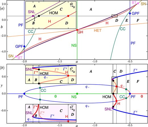
One encounters a one-parameter sequence of bifurcations in system (1.10) that is somewhat typical for planar systems with discrete rotational symmetry. It is found along a straight path of the two-parameter bifurcation set of (1.10) in the |$(a, b)$|-plane. Figure 1(a) shows the two-parameter bifurcation set and panel (|$b$|) the corresponding one-parameter bifurcation diagram through regions |$\boldsymbol {A}--\boldsymbol {F}$|.
Regions A–F of topologically different phase portraits of system (1.10) for |$c=2.5$| and |$d=2.5$|. Panel (|$a$|) shows the two-parameter bifurcation diagram in the |$(a,b)$|-plane with the bifurcation curves: Hopf ( ), saddle-node of limit cycle (
 ), homoclinic |$(\textbf {\texttt {HOM}})$|, heteroclinic (
 ), saddle-node of equilibria (
 ) and pitchfork (
 ); and filled circles marking the codimension-two points: generalized Hopf (
 ), generalized pitchfork (
 ) and Bogdanov–Takens (
 ). We further show the locus
  where
where  is a neutral saddle, and the locus
  at which the nontrivial equilibria |$q_{\pm }$| have a complex-conjugate pair of eigenvalues with zero imaginary part. Panel (|$b$|) shows the one-parameter bifurcation diagram in the |$(a,y)$|-plane for |$b=0.5$| (indicated by the thick horizontal gray line in panel (|$a$|), with regions |$\boldsymbol {A}-\boldsymbol {F}$| demarcated by thin gray lines; periodic orbits are represented by their extremal values in |$y$|. The equilibria |$q_{\pm }$| and |$\boldsymbol {0}$|, and the periodic orbits
  ,
,  and
and  are coloured blue, red or green, depending on whether they are attracting, repelling or of saddle type, respectively. The inset in panel (|$a$|) is an enlargement in the |$(a,b)$|-plane of the highlighted box over a range in |$a$| that illustrates the regions |$\boldsymbol {A}-\boldsymbol {D}$| along |$b=0.5$|. The insets in panel (|$b$|) share that same |$a$|-range; the upper inset shows the enlargement in the |$(a,y)$|-plane of the highlighted box, and the lower inset shows the |$(a,\mathrm {T}_{})$|-plane.
The overall bifurcation structure in the |$(a, b)$|-plane is invariant under rotation by |$\pi $| around the point |$(a, b) = ({-c}/ {2}, {-d}/ {2})$|, which is the result of the invariance of (1.10) under |$(a, b) \mapsto (-a - c, -b - d)$| and |$(x, y) \mapsto (-y, -x)$|. Hence, the bifurcation set is invariant under the spatio-temporal symmetry of reflection of the phase portrait in the diagonal (where |$x=y$|) and time reversal. At the central point at |$(a, b) = (-1.25, -1.25)$| of the rotational symmetry in Fig. 1(|$a$|) (where |$c=2.5$| and |$d=2.5$|) the system is reversible. Most bifurcation curves come together and change criticality at this central point, which we refer to as |$\textbf {\texttt {GH}}$|. Hence, together with a symmetric pair of Bogdanov–Takens bifurcation points |$\textbf {\texttt {BT}}$|, the point |$\textbf {\texttt {GH}}$| acts as an organizing centre for the bifurcation diagram in the |$(a, b)$|-plane of (1.10).
Due to the symmetry of Fig. 1((a)), we describe the bifurcation structure only for parameters |$(a,b)$| to the right of the vertical line |$\textbf {\texttt {NS}}$| (through |$\textbf {\texttt {GH}}$|) along which the origin |$\boldsymbol {0}$| is a neutral saddle. The point |$\textbf {\texttt {GH}}$| marks a transition from supercritical to subcritical bifurcation along the curve |$\textbf {\texttt {HB}}$| of Hopf bifurcations of a symmetric pair of nontrivial equilibria |$q_{\pm }$| Three further curves emerge from |$\textbf {\texttt {GH}}$|: a homoclinic bifurcation |$\textbf {\texttt {HOM}}$| involving the invariant manifolds of the origin |$\boldsymbol {0}$|, a saddle-node bifurcation |$\textbf {\texttt {SNL}}$| of limit cycles |$\varGamma ^{s}$| and |$\varGamma ^u$| and a heteroclinic bifurcation |$\textbf {\texttt {HET}}$| involving the invariant manifolds of a symmetric pair of saddle points |$p_{\pm }$|. 5 The curves |$\textbf {\texttt {HB}}$| and |$\textbf {\texttt {HOM}}$| both terminate at the point |$\textbf {\texttt {BT}}$| on the curve |$\textbf {\texttt {SN}}$| of saddle-node bifurcations (of |$q{\pm }$| and |$p^0_{\pm }$|, introduced below). To the right of |$\textbf {\texttt {BT}}$| the curve |$\textbf {\texttt {SN}}$| terminates at the generalized pitchfork bifurcation point |$\textbf {\texttt {GPF}}$| on the vertical line |$\textbf {\texttt {PF}}$| of pitchfork bifurcation of |$\boldsymbol {0}$|. The criticality of |$\textbf {\texttt {PF}}$| changes at |$\textbf {\texttt {GPF}}$|. For fixed |$b$| below |${\textbf {\texttt {GPF}}}$|, the repelling equilibria |$q_{\pm }$| disappear at |$\textbf {\texttt {PF}}$| as |$a$| increases, while for fixed |$b$| above |$\textbf {\texttt {GPF}}$| the saddle points |$p^0_{\pm }$| are created, instead. The curve |$\textbf {\texttt {SNL}}$| terminates at the curve |$\textbf {\texttt {HOM}}$| at a point of noncentral homoclinic saddle-node bifurcation that exists too close to |$\textbf {\texttt {BT}}$| to be pictured in panel (|$a$|). To the right of this point and along |$\textbf {\texttt {SN}}$|, the saddle-node bifurcation of the equilibria |$p^0_{\pm }$| and |$q_{\pm }$| occurs on |$\varGamma ^{s}$|. The relative order of the three bifurcation curves |$\textbf {\texttt {SNL}}$|, |$\textbf {\texttt {HOM}}$| and |$\textbf {\texttt {HB}}$| is illustrated in the inset at the top of panel (|$a$|), which is an enlargement of the corresponding framed region to the right and along the gray line.
From left to right along the gray line in Fig. 1((a)), the attracting periodic orbit |$\varGamma ^{s}$| and the repelling periodic orbit |$\varGamma ^u$| are created as |$\textbf {\texttt {SNL}}$| is crossed; then |$\varGamma ^u$| transitions into the pair of repelling periodic orbits |$\varGamma ^u_{\pm }$| at the curve |$\textbf {\texttt {HOM}}$|; finally, at |$\textbf {\texttt {HB}}$| the pair |$\varGamma ^u_{\pm }$| disappear. Also shown is the curve |$(\textbf {\texttt {CC}})$| where the eigenvalues of |$q_{\pm }$| become complex conjugate. 6 Considering the isochrons of |$q_{\pm }$|, defined as discussed in Section 1.3, the curve |$(\textbf {\texttt {CC}})$| marks the boundary between their existence (to the left) and nonexistence (to the right). This curve passes through |$\textbf {\texttt {BT}}$| tangent to |$\textbf {\texttt {HB}}$|, and continues out of the frame above |$\textbf {\texttt {SN}}$|. Finally, the curve |$\textbf {\texttt {HET}}$| leaves the frame to the right and is not part of the bifurcation sequence that we consider.
Along the gray line given by |$b = 0.5$| in Fig. 1((a)) we find the bifurcation sequence: |$\textbf {\texttt {PF}}$|, |$(\textbf {\texttt {CC}})$|, |$\textbf {\texttt {SNL}}$|, |$\textbf {\texttt {HOM}}$|, |$\textbf {\texttt {HB}}$|, |$(\textbf {\texttt {CC}})$| and |$\textbf {\texttt {PF}}$|, in that order, as |$a$| is increased. We record the values of |$a$| at which the bifurcations in this sequence are encountered in Table 1. Figure 1(|$b$|) shows the associated one-parameter bifurcation diagram, where the maximum and minimum |$y$|-values of the respective invariant objects are shown as a function of |$a$|; notice the symmetry of reflection in |$y = 0$|. This bifurcation sequence gives rise to the regions |$\boldsymbol {A}--\boldsymbol {F}$| of different phase portraits. Specifically, we first encounter the pitchfork bifurcation |$\textbf {\texttt {PF}}$| of the origin |$\boldsymbol {0}$| at |$a=-2$|, which generates the nodal attractors |$q_{\pm }$|. When |$a$| is increased through |$a \approx -1.778$|, the curve |$(\textbf {\texttt {CC}})$| is crossed and |$q_{\pm }$| transform into attracting foci. While one would not consider |$(\textbf {\texttt {CC}})$| a bifurcation, it is the first point along this bifurcation sequence past which isochrons can be defined. Thus, the resulting region |$\boldsymbol {A}$| is the first of the six regions |$\boldsymbol {A}--\boldsymbol {F}$| in panels (|$a$|)and (|$b$|) of Fig. 1. The associated structurally stable two-dimensional phase portraits in the |$(x, y)$|-plane are shown in Fig. 2 and described in Section 2.1.
Parameter values of |$a$| at which the bifurcations occur for |$b=0.5$|; see also Fig. 1((b)). All values are approximate unless given to fewer than three decimal places.
 |
|
Parameter values of |$a$| at which the bifurcations occur for |$b=0.5$|; see also Fig. 1((b)). All values are approximate unless given to fewer than three decimal places.
|
|
Representative phase portraits of (1.10) showing the invariant objects in the topologically different regions A–F as described in Fig. 1(|$a$|). Sources, saddles and sinks are represented by  ,
,  and
and  , respectively, with equilibria and periodic orbits coloured and labelled as described in Fig. 1. Also shown are the stable manifolds
  (light-blue curve) and the unstable manifolds
  (orange curve), and the strong unstable manifold
  (orange) in region |$\boldsymbol {F}$|. The basins of attraction (
 ) and repulsion (
 and
and  ) of the left invariant object in a symmetric pair of equilibria or periodic orbits are shaded green and pink, respectively.
As |$\textbf {\texttt {SNL}}$| is crossed at |$a \approx -0.746$|, the periodic orbits |$\varGamma ^{s}$| and |$\varGamma ^u$| are created. They exist in region |$\boldsymbol {B}$|, and are symmetric, surrounding all equilibria shown. Region |$\boldsymbol {B}$| only exists after |$\textbf {\texttt {SNL}}$| for a relatively short |$a$|-interval up to |$\textbf {\texttt {HOM}}$|; see the enlargement with the bifurcations |$\textbf {\texttt {SNL}}$|, |$\textbf {\texttt {HOM}}$| and |$\textbf {\texttt {HB}}$| (top inset), and the periods of the periodic orbits |$\varGamma ^{s}$|, |$\varGamma ^u$| and |$\varGamma ^u_-$|, respectively (bottom inset). Also shown is the natural period of the equilibrium |$q_{-}$|, which is tangent to that of |$\varGamma ^u_-$| at |$\textbf {\texttt {HB}}$|. Note that the horizontal |$a$|-axes are aligned for each of panels (|$a$|)and (|$b$|) and, likewise, for their insets.
The bottom inset of Fig. 1((b)) clearly shows that, as the symmetric homoclinic bifurcation |$\textbf {\texttt {HOM}}$| is approached, the period of |$\varGamma ^u$| tends to |$\infty $|, and a pair of nonsymmetric repelling periodic orbits |$\varGamma ^u_{\pm }$| is created and exist in region |$\boldsymbol {C}$|; 7 for decreasing |$a$|, one also speaks of a gluing bifurcation of the two periodic orbits |$\varGamma ^u_{\pm }$| to create the periodic orbit |$\varGamma ^u$|. The periods of |$\varGamma ^u_{\pm }$| also tend to |$\infty $| as |$\textbf {\texttt {HOM}}$| is approached for decreasing |$a$|. Region |$\boldsymbol {C}$| is bounded by |$\textbf {\texttt {HOM}}$| and a symmetric pair of Hopf bifurcations |$\textbf {\texttt {HB}}$| at |$a\approx -0.691$|, in which |$\varGamma ^u_{\pm }$| disappear and |$q_{\pm }$| change stability from sink to source. This leaves the periodic orbit |$\varGamma ^{s}$| as the only attractor in region |$\boldsymbol {D}$|. After crossing the second curve |$(\textbf {\texttt {CC}})$| into region |$\boldsymbol {E}$|, the repelling equilibria |$q_{\pm }$| lose their innate rotation and no phase related to |$q_{\pm }$| can be assigned in region |$\boldsymbol {E}$| and beyond. Region |$\boldsymbol {F}$| lies to the right of the final pitchfork bifurcation |$\textbf {\texttt {PF}}$| at |$a=-0.5$|, in which the two equilibria |$q_{\pm }$| disappear. This leaves only the nodal source |$\boldsymbol {0}$| surrounded by the attracting periodic orbit |$\varGamma ^{s}$|.
Note that we are not considering the regions between |$\textbf {\texttt {GPF}}$| and |$\textbf {\texttt {BT}}$| at the top right-hand side of Fig. 1((a)) in this case study. At the bifurcation curve |$\textbf {\texttt {PF}}$| an additional pair of saddle points |$p^0_{\pm }$| emanates from the repelling equilibria at the origin |$\boldsymbol {0}$|, which then collide with the sources |$q_{\pm }$| at |$\textbf {\texttt {SN}}$|. Apart from this, the respective regions to the right of |$\textbf {\texttt {PF}}$| are quite similar to the regions |$\boldsymbol {A}-\boldsymbol {F}$|. Namely, in each case, the bifurcations and dynamics along the bifurcation sequence that we are considering are preserved.
2.1 Phase portraits
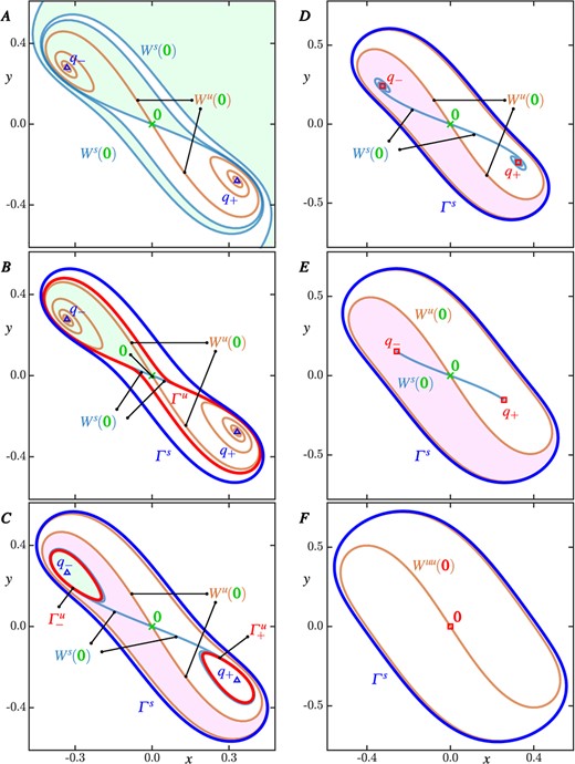
As the starting point for our investigation of isochron foliations, Fig. 2 shows representative phase portraits in regions |$\boldsymbol {A}-\boldsymbol {F}$|, for the values of |$a$| recorded in Table 2. In these and all following phase portraits, we include all relevant invariant objects. The origin is always an equilibrium; attracting, repelling, and saddle-type equilibria are represented by triangles ( ), squares (
 ) and crosses (
 ), respectively. Stable and unstable invariant manifolds of saddle equilibria are denoted |$W^s(\cdot )$| and |$W^u(\cdot )$|, respectively, and periodic orbits are labelled |$\varGamma ^{s}$|, |$\varGamma ^u$| and |$\varGamma ^u_{\pm }$|, (as before) where the superscript denotes stability. Basins of attraction |$\mathcal {A}\left ({\cdot }\right )$| and basins of repulsion |$\mathcal {R}(\cdot )$|, respectively, may come as pairs belonging to equilibria and periodic orbits that are symmetrically related by rotation over |$\pi $|. In such cases, the basin of attraction of the left-most equilibrium is shaded green, and the basin of repulsion of the left-most equilibrium or periodic orbit is shaded pink.
| Region | |$\boldsymbol {A}$| | |$\boldsymbol {B}$| | |$\boldsymbol {C}$| | |$\boldsymbol {D}$| | |$\boldsymbol {E}$| | |$\boldsymbol {F}$| |
|---|---|---|---|---|---|---|
| |$a$| | -0.75 | -0.742 | -0.71 | -0.66 | -0.55 | -0.45 |
| Region | |$\boldsymbol {A}$| | |$\boldsymbol {B}$| | |$\boldsymbol {C}$| | |$\boldsymbol {D}$| | |$\boldsymbol {E}$| | |$\boldsymbol {F}$| |
|---|---|---|---|---|---|---|
| |$a$| | -0.75 | -0.742 | -0.71 | -0.66 | -0.55 | -0.45 |
| Region | |$\boldsymbol {A}$| | |$\boldsymbol {B}$| | |$\boldsymbol {C}$| | |$\boldsymbol {D}$| | |$\boldsymbol {E}$| | |$\boldsymbol {F}$| |
|---|---|---|---|---|---|---|
| |$a$| | -0.75 | -0.742 | -0.71 | -0.66 | -0.55 | -0.45 |
| Region | |$\boldsymbol {A}$| | |$\boldsymbol {B}$| | |$\boldsymbol {C}$| | |$\boldsymbol {D}$| | |$\boldsymbol {E}$| | |$\boldsymbol {F}$| |
|---|---|---|---|---|---|---|
| |$a$| | -0.75 | -0.742 | -0.71 | -0.66 | -0.55 | -0.45 |
The phase portrait in region A in Fig. 2 has a symmetric pair of attracting focus-type equilibria |$q_{\pm }$| that are the end points of the unstable manifold |$W^u(\boldsymbol {0})$| of the origin |$\boldsymbol {0}$|. The stable manifold |$W^s(\boldsymbol {0})$| of |$\boldsymbol {0}$| separates the basins of attraction |$\mathcal {A}\left (q_{-}\right )$| (shaded) and |$\mathcal {A}\left (q_{+}\right )$|; its two branches wind anti-clockwise around |$\boldsymbol {0}$| and |$q_{\pm }$|, and tend towards infinity in backward time. Hence, the finite portion of the boundaries |$\partial \mathcal {A}\left (q_{\pm }\right )$| of the basins of attraction |$\mathcal {A}(q_{\pm })$| are formed by |$\boldsymbol {0}$| and its stable manifold |$W^s(\boldsymbol {0})$|.
The phase portrait in region B, after |$\textbf {\texttt {SNL}}$| has been crossed, shows the pair of nested periodic orbits |$\varGamma ^{s}$| (outer) and |$\varGamma ^u$| (inner) that surround the other invariant objects. The stable manifold |$W^s(\boldsymbol {0})$|, forming the basin boundaries |$\partial \mathcal {A}\left (q_{\pm }\right )$|, now forms a double spiral that accumulates onto |$\varGamma ^u$| in backward time so that the basins |$\mathcal {A}\left (q_{-}\right )$| (shaded) and |$\mathcal {A}\left (q_{+}\right )$| are now contained inside of |$\varGamma ^u$|. We refer to |$\mathcal {A}\left (q_{\pm }\right )$| as winding basins and remark that their boundary, the closure |$\overline {W^s(\boldsymbol {0})}$|, which contains |$\varGamma ^u$|, is a complete metric space that is not path-connected. More specifically, each branch of |$W^s(\boldsymbol {0})$| is a closed outward spiral that accumulates on the topological circle |$\varGamma ^u$| (see, for example, Pugh, 2002, Figure 22 for a sketch), and |$W^s(\boldsymbol {0})$| is, hence, a closed double spiral that accumulates on a circle—akin to the well-known Yin and Yang symbol. Notice that |$W^s(\boldsymbol {0})$| approaches |$\varGamma ^u$| very rapidly such that only an initial piece of |$W^s(\boldsymbol {0})$| can be seen in the phase portrait of region |$\boldsymbol {B}$| in Fig. 2. The area between the periodic orbits |$\varGamma ^{s}$| and |$\varGamma ^u$| is an annulus, where |$\mathcal {A}\left ({\varGamma ^{s}}\right )$| and |$\mathcal {R}{\varGamma ^u}$| coincide. The basin of repulsion |$\mathcal {R}{\varGamma ^u}$| is bounded inside |$\varGamma ^u$| by the unstable manifold |$W^s(\boldsymbol {0})$| and the equilibria |$q_{\pm }$| on which |$W^s(\boldsymbol {0})$| accumulates. Notice that |$\mathcal {R}{\varGamma ^u}$| covers the basins of attraction |$\mathcal {A}\left (q_{\pm }\right )$| of the attracting equilibria |$q_{\pm }$| except for the set |$W^u(\boldsymbol {0}) \setminus \boldsymbol {0} \subset \mathcal {A}\left (q_{-}\right ) \cup \mathcal {A}\left (q_{+}\right )$|, while the basins |$\mathcal {A}\left (q_{\pm }\right )$| cover |$\mathcal {R}{\varGamma ^u}$| inside |$\varGamma ^u$| except for the set |$W^s(\boldsymbol {0}) \setminus \boldsymbol {0} \subset \mathcal {R}{\varGamma ^u}$|.
In region C of Fig. 2, after |$\textbf {\texttt {HOM}}$| has been crossed, there are now three periodic orbits: the attracting periodic orbit |$\varGamma ^{s}$| surrounds a symmetric pair of repelling periodic orbits |$\varGamma ^u_{\pm }$|. The basins of attraction |$\mathcal {A}\left (q_{-}\right )$| (shaded) and |$\mathcal {A}\left (q_{+}\right )$| are bounded by |$\varGamma ^u_-$| and |$\varGamma ^{u}_{+}$|, respectively. Moreover, the branches of the stable manifold |$W^s(\boldsymbol {0})$| each accumulate onto one of |$\varGamma ^u_-$| and |$\varGamma ^{u}_{+}$| in backward time. The unstable manifold |$W^u(\boldsymbol {0})$| forms the boundary between the basins of repulsion |$\mathcal {R}{\varGamma ^u_-}$| (shaded) and |$\mathcal {R}{\varGamma ^u_+}$|, together with the attracting periodic orbit |$\varGamma ^{s}$| on which it accumulates in forward time. Hence, the closure |$\overline {W^u(\boldsymbol {0})}$| is not path-connected, contains |$\varGamma ^{s}$| and bounds the two winding basins of repulsion |$\mathcal {R}{\varGamma ^u_{\pm }}$|. The basin of attraction |$\mathcal {A}\left ({\varGamma ^{s}}\right )$| outside |$\varGamma ^{s}$| extends to infinity, and inside |$\varGamma ^{s}$| its boundary |$\partial \mathcal {A}\left ({\varGamma ^{s}}\right )$| is the closure |$\overline {W^s(\boldsymbol {0})}$|, which contains |$\varGamma ^u_{\pm }$| and is not path-connected. Hence, at |$\textbf {\texttt {HOM}}$| where the invariant manifolds |$W^s(\boldsymbol {0})$| and |$W^u(\boldsymbol {0})$| pass through each other, the geometry of the winding basins switches. The basin |$\mathcal {A}\left ({\varGamma ^{s}}\right )$| covers the pair of winding basins of repulsion |$\mathcal {R}{\varGamma ^u_{\pm }}$| of the two periodic orbits |$\varGamma ^u_{\pm }$|, except for the set |$W^s(\boldsymbol {0}) \setminus \boldsymbol {0} \subset \mathcal {R}{\varGamma ^u_-} \cup \mathcal {R}{\varGamma ^u_+}$|, while the basins |$\mathcal {R}{\varGamma ^u_{\pm }}$| cover |$\mathcal {A}\left ({\varGamma ^{s}}\right )$| inside |$\varGamma ^u$|, except for the set |$W^u(\boldsymbol {0}) \setminus \boldsymbol {0} \subset \mathcal {A}\left ({\varGamma ^{s}}\right )$|.
In region D, after the transition through |$\textbf {\texttt {HB}}$|, the periodic orbits |$\varGamma ^u_{\pm }$| have disappeared and |$q_{\pm }$| are now repelling foci. The origin |$\boldsymbol {0}$| remains a saddle-type equilibrium, and the basins of attraction |$\mathcal {A}\left (q_{-}\right )$| (shaded) and |$\mathcal {A}\left (q_{-}\right )$| are bounded by |$W^u(\boldsymbol {0})$| and |$\varGamma ^{s}$|, onto which each branch of |$W^u(\boldsymbol {0})$| accumulates in forward time. The basin boundary |$\partial \mathcal {A}\left ({\varGamma ^{s}}\right )$| is again the closure |$\overline {W^s(\boldsymbol {0})}$|, but now this is a curve of finite arclength containing |$q_{\pm }$| and |$\boldsymbol {0}$|; hence, |$\partial \mathcal {A}\left ({\varGamma ^{s}}\right )$| is path connected and |$\mathcal {A}\left ({\varGamma ^{s}}\right )$| inside |$\varGamma ^{s}$| is topologically an annulus. The basin boundary |$\partial \mathcal {R}(q_{\pm })$|, which is the closure of |$W^u(\boldsymbol {0})$| containing |$\varGamma ^{s}$|, is not path connected. The basin |$\mathcal {A}\left ({\varGamma ^{s}}\right )$| still covers two winding basins of repulsion, namely, |$\mathcal {R}(q_{\pm })$|, except for the set |$W^s(\boldsymbol {0}) \setminus \boldsymbol {0} \subset \mathcal {R}(q_{-}) \cup \mathcal {R}(q_{+})$|.
The phase portrait in region E of Fig. 2, after |$(\textbf {\texttt {CC}})$| has been crossed, is topologically equivalent to that in region D. However, for our purposes, it is significant that in region |$\boldsymbol {E}$| the equilibria |$q_{\pm }$| do not have an innate rotation, so that one cannot assign an associated phase to them any longer. In particular, the boundary |$\partial \mathcal {A}\left ({\varGamma ^{s}}\right )$| of the basin |$\mathcal {A}\left ({\varGamma ^{s}}\right )$| is still the closure |$\overline {W^{s}(\boldsymbol {0})}$|, but this manifold does not spiral any longer; rather its branches approach each |$q_{\pm }$|, respectively, from unique directions, namely, along the weak eigendirections of these nodal equilibria.
In region F, after |$\textbf {\texttt {PF}}$| has been crossed, the equilibria |$q_{\pm }$| disappear, leaving the origin |$\boldsymbol {0}$|, which is now a nodal repellor, as the only equilibrium inside |$\varGamma ^{s}$|. In the representative phase portrait for region |$\boldsymbol {F}$| in Fig. 2, we plot the well-defined and unique strong unstable manifold |$W^{uu}(\boldsymbol {0})$|, which is the counterpart of the unstable invariant manifolds |$W^{u}(\boldsymbol {0})$| in regions |$\boldsymbol {A}-\boldsymbol {E}$|. The basin of attraction |$\mathcal {A}\left ({\varGamma ^{s}}\right )$| inside |$\varGamma ^{s}$| is now the annulus bounded by the point |$\boldsymbol {0}$|.
We remark that phase portraits topologically equivalent to those in regions E and F have been investigated in terms of the related concepts of phase-response (Borek et al., 2011) and isochrons (Glass & Winfree, 1984); how the forward-time isochrons accumulate on the basin boundary (including infinity) for these two cases with saddle equilibria in the basin boundary was first illustrated with actual computations by Hannam et al. (2016). These earlier works motivated the case study presented here, where we focus on transversality properties of the foliations by both forward-time and backward-time isochrons during the entire, more complicated transition through regions |$\boldsymbol {A}-\boldsymbol {F}$|.
3. Isochron geometry in regions A to F
We now discuss how the isochron foliations and their interactions, in the different basins of attraction and repulsion where they exist, change with the parameter |$a$| along the bifurcation sequence. In particular, we are interested in the existence of sharp turns in an isochron foliation and related tangencies between forward-time and backward-time isochron foliations. Because every isochron must pass arbitrarily close to each point on the boundary of the basin of attraction or repulsion that it belongs to (Guckenheimer, 1975; Winfree, 1974), the geometric properties of these boundaries (described in Section 2.1) and how isochrons accumulate onto them are particularly important. For each representative phase portraits of regions |$\boldsymbol {A}-\boldsymbol {F}$|, we compute a selection of forward-time and/or backward-time isochrons of the relevant periodic orbits and focus-type equilibria; more specifically, for each of a symmetric pair of periodic orbits or foci we show ten isochrons uniformly distributed in phase, and for symmetric periodic orbits we show twenty such isochrons.
We first present in Section 3.1 an overview of the isochron geometry in each of regions |$\boldsymbol {A}-\boldsymbol {F}$|; here, we mention the types of basins in which isochrons are encountered and provide a very brief discussion of the changes to the isochron foliations from region to region. An in-depth explanation of the properties of each isochron foliation in each region is presented in Sections 3.2 to 3.6. Since the geometry of the isochrons and their interactions can be rather subtle, we present them there in different ways. To make optimal use of space, we will show phase portraits rotated around |$\boldsymbol {0}$| by |$0.3 \pi $| in the counter-clockwise direction; we refer to this representation as the |$(v, w)$|-plane and we choose to preserve the asymptotic phase under this rotation, that is, the zero-phase point |$\gamma _{0}$| is also rotated by |$0.3 \pi $|. Each isochron is computed and represented as a curve parametrized by its arclength |$\ell $|—as measured from the equilibrium for isochrons of equilibria, and from the point |$\gamma _{\theta }$| on the periodic orbit for isochrons of periodic orbits. This allows us to show the geometry of computed isochrons not only in phase space, but also as a function of arclength |$\ell $|, as a way to emphasize an isochron’s complex geometry. Here, we use the sign convention that |$\ell $| is positive for the branch of the isochron that lies outside the periodic orbit, and negative for the branch of the isochron that lies inside the periodic orbit. Finally, we will provide sketches to illustrate topological and geometrical properties of certain isochrons and, especially, how they accumulate onto the boundaries of their basins.
3.1 Overview of isochron foliations
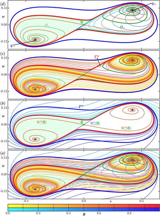
Figure 3 shows the same phase portraits as Fig. 2 of regions |$\boldsymbol {A}-\boldsymbol {F}$| in descending order across its columns, but now each panel also shows all forward-time and backward-time isochron foliations that exist in these regions; these are |$\mathcal {I}\left (q_{\pm }\right )$| in regions |$\boldsymbol {A}-\boldsymbol {B}$| and |$\mathcal {I}\left (\varGamma ^{s}\right )$| in regions |$\boldsymbol {B}-\boldsymbol {F}$|, as well as |$\mathcal {U}(\varGamma ^u)$| in region |$\boldsymbol {B}$|, |$\mathcal {U}(\varGamma ^u_{\pm })$| in region |$\boldsymbol {C}$|, and |$\mathcal {U}(q_{\pm })$| in regions |$\boldsymbol {C}-\boldsymbol {D}$|. Hence, there are interactions between isochron foliations only in regions |$\boldsymbol {B}-\boldsymbol {D}$|, where both forward-time and backward-time isochron foliations coexist. In this and all following figures, forward-time isochrons are represented by curves coloured in tones between cyan and blue, and backward-time isochrons by curves coloured in tones between yellow and red. These colours indicate the phase |$\theta $| of an isochron of the respective foliation as per the respective colour bar at the bottom of Figure 3.
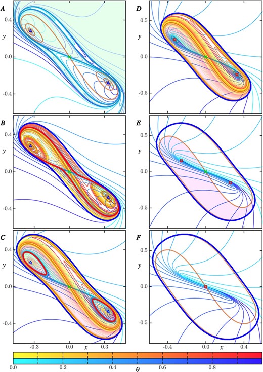
Phase portraits from Fig. 2 overlaid with the forward-time and backward-time isochron foliations of their respective eligible invariant objects. Twenty and ten isochrons, equally distributed in phase |$\theta $|, are shown for each foliation of symmetric and pairwise-symmetric objects, respectively; each isochron is coloured according to its phase in either forward or backward time as given by the lower and upper colour bars.
The phase portrait for region A in Fig. 3 shows the isochron foliations |$\mathcal {I}\left (q_{\pm }\right )$| of |$q_{\pm }$|, which are the only objects with oscillatory behaviour. Observe how each isochron |$I_{\theta }(q_{\pm }) \in \mathcal {I}\left (q_{\pm }\right )$| spirals away from the respective equilibrium |$q_{\pm }$|, resulting in sharp turns as the basins |$\mathcal {A}\left (q_{\pm }\right )$| are wound to become more elongated. Note the regions of extreme phase sensitivity where |$W^s(\boldsymbol {0})$| passes very close to itself.
The saddle-node bifurcation |$\textbf {\texttt {SNL}}$| produces two periodic orbits in region B, where the outer attracting periodic orbit |$\varGamma ^{s}$| encloses the repelling orbit |$\varGamma ^u$|. In the annulus between them the forward-time isochron foliation |$\mathcal {I}\left (\varGamma ^{s}\right )$| of |$\varGamma ^{s}$| intersects the backward-time isochron foliation |$\mathcal {U}(\varGamma ^u)$| of |$\varGamma ^u$| transversely everywhere. We denote such a transverse intersection of isochron foliations by |$\mathcal {I}\left (\varGamma ^{s}\right )$| |$\mathcal {U}(\varGamma ^u)$|. The forward-time isochron foliations |$\mathcal {I}\left (q_{\pm }\right )$| are now restricted to the pair of winding basins |$\mathcal {A}\left (q_{\pm }\right )$| that accumulate onto |$\varGamma ^u$|. The backward-time isochron foliation |$\mathcal {U}(\varGamma ^u)$| exists inside of |$\varGamma ^u$|; it exhibits sharp turns that are tangent to the forward-time isochrons in |$\mathcal {I}\left (q_{\pm }\right )$|. The existence of nontransverse (tangential) intersections between these foliations is denoted by |$\mathcal {I}\left (q_{\pm }\right )$|
 |$\mathcal {U}(\varGamma ^u$|. An isochron |$U_{\theta }(\varGamma ^u) \in \mathcal {U}(\varGamma ^u)$| must accumulate onto |$\overline {W^u(\boldsymbol {0})} = q_{\pm } \cup W^u(\boldsymbol {0}) \cup \boldsymbol {0}$|. The exact manner in which this happens is hard to see in Figure 3 and will be discussed in detail in Section 3.3.
In region C, the homoclinic bifurcation |$\textbf {\texttt {HOM}}$| has led to a dramatic change of the invariant sets and their basins. The backward-time isochron foliations |$\mathcal {U}(\varGamma ^u_{\pm })$| of the pair of symmetric orbits |$\varGamma ^u_{\pm }$| have clear sharp turns while they accumulate onto both branches of |$W^u(\boldsymbol {0})$| that form the boundaries |$\partial \mathcal {R}(\varGamma ^u_{\pm })$| of the winding basins of repulsion |$\mathcal {R}(\varGamma ^u_{\pm })$|. At the same time, the forward-time isochrons |$I_{\theta }\left ({\varGamma ^{s}}\right )$| have developed sharp turns as well, but these are very hard to see in Figure 3. As we will show in detail in Section 3.4, these two isochron foliations have tangential intersections, that is, |$\mathcal {I}\left ({\varGamma ^{s}}\right )$||$\mathcal {U}(\varGamma ^u_{\pm })$|. In contrast, the isochron geometry in the annuli |$\mathcal {A}\left (q_{\pm }\right )$| is much simpler: the two foliations intersect transversely, that is, |$\mathcal {A}\left (q_{\pm }\right )$||$\mathcal {U}(\varGamma ^u_{\pm })$|.
In region D, the pair of repelling periodic obits has shrunk down to the points |$q_{\pm }$|, which are now spiralling repellors. As Fig. 3 shows, they inherit the properties of the isochron foliations of the periodic orbits, meaning that |$\mathcal {I}\left (\varGamma ^{s}\right )$||$\mathcal {U}(q_{\pm })$|. Here, the foliations |$\mathcal {U}(q_{\pm })$| exist in the pair of winding basins of repulsion |$\mathcal {R}(q_{\pm })$|, and also show sharp turns associated with their tangencies with |$\mathcal {I}\left (\varGamma ^{s}\right )$|. This will be discussed in detail in Section 3.5.
In regions E and F, past the curve |$(\textbf {\texttt {CC}})$|, there is only the foliation by forward-time isochrons of the basin |$\mathcal {A}\left ({\varGamma ^{s}}\right )$|. While the transition from regions |$\boldsymbol {D}--\boldsymbol {E}$| does not constitute a topological change, the isochron geometry of |$\mathcal {I}\left (\varGamma ^{s}\right )$| changes significantly. In region |$\boldsymbol {E}$|, the isochrons in |$I_{\theta }\left ({\varGamma ^{s}}\right )$| accumulate onto the closed curve |$\overline {W^s(\boldsymbol {0})} = W^s(\boldsymbol {0}) \cup q_{\pm }$| by spiralling around this curve, getting closer with each pass as their arclengths increase. In particular, the foliation |$I_{\theta }\left ({\varGamma ^{s}}\right )$| in region |$\boldsymbol {E}$| no longer features sharp turns. In region |$\boldsymbol {F}$| the isochrons of |$I_{\theta }\left ({\varGamma ^{s}}\right )$| accumulate onto the single point |$\boldsymbol {0}$|, but Figure 3 shows that there is still a somewhat extended region of phase sensitivity near the slow eigenspace of |$\boldsymbol {0}$|.
3.2 Isochrons in region A
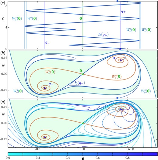
In region A, there are only the two symmetrically related foliations |$\mathcal {I}\left (q_{\pm }\right )$| of forward-time isochrons of |$q_{\pm }$| that exist in the two basins |$\mathcal {A}\left (q_{\pm }\right )$|. Their geometry is illustrated in Figure 4 in three different ways. Panel (|$a$|) shows an enlargement of the phase portrait in the (rotated) |$(v, w)$|-plane, consisting of the attractors |$q_{\pm }$|, the saddle |$\boldsymbol {0}$| and its stable and unstable manifolds |$W^s(\boldsymbol {0})$| and |$W^u(\boldsymbol {0})$|, together with ten isochrons of |$\mathcal {I}\left (q_{+}\right )$| that are distributed uniformly spaced in phase. Panel (|$b$|) shows the same phase portrait with only the zero-phase isochron |$I_{0}(q_{+})$|, and panel (|$c$|) is a representation of |$I_{0}(q_{+})$| in terms of its arclength |$\ell $| versus the |$v$|-coordinate.
Details of isochron geometry in region A in the (rotated) |$(v, w)$|-plane. Panel ((a)) shows the phase portrait, consisting of  ,
,  and
and  and
and  , together with ten isochrons of (
 ), and panel (|$b$|) shows the phase portrait with only the zero-phase isochron
  ; here, each isochron in panel (|$a$|) is coloured according to its phase |$\theta $| as given by the colour bar. Panel (|$c$|) shows how the |$v$|-coordinate along
  changes with arclength |$\ell $|, where the |$v$|-range is as in panels (|$a$|)and(|$b$|) and the vertical lines indicate the positions
  ,
,  and the folds of
  with respect to the |$v$|-direction. Compare with Figs. 2 and 3.
Figure 4(a) shows clearly how the ten isochrons intersect |$W^u(\boldsymbol {0})$| transversely near |$q_{+}$|; in particular, this implies that each isochron in |$\mathcal {I}\left (q_{+}\right )$| accumulates onto |$W^s(\boldsymbol {0})$| locally near |$\boldsymbol {0}$|. The basin |$\mathcal {A}\left (q_{+}\right )$|, including its boundary, extends to infinity; since isochrons must accumulate onto the entirety of the basin that they foliate (Guckenheimer, 1975), each isochron also needs to grow beyond bound while accumulating on both branches of |$W^s(\boldsymbol {0}) \subset \partial \mathcal {A}\left (q_{+}\right )$|, which we denote |$W^s_{-}(\boldsymbol {0})$| and |$W^s_{+}(\boldsymbol {0})$| as indicated in Figure 4. In the process, the isochrons switch over from one branch of |$W^s(\boldsymbol {0})$| to its other branch, specifically from |$W^s_{-}(\boldsymbol {0})$| to |$W^s_{+}(\boldsymbol {0})$|; notice how this leads to quite sharp turns of the isochrons in Fig. 4(|$a$|)where they need to ‘squeeze through’ the narrow channel where the two branches of |$W^s(\boldsymbol {0})$| come very close to each other. Indeed, the turns are much less sharp once they occur past this narrow channel.
Figure 4(b) illustrates the geometry for just |$I_{0}(q_{+})$|. Notice how this curve approaches and follows first |$W^s_{+}(\boldsymbol {0})$| and then |$W^s_{-}(\boldsymbol {0})$| after a close pass of |$\boldsymbol {0}$|; it then makes a turn to switch back to |$W^s_{+}(\boldsymbol {0})$|, which it now follows even more closely; after an even closer pass of |$\boldsymbol {0}$|, it again follows |$W^s_{-}(\boldsymbol {0})$|, all the way through the narrow channel, before making the next switch back to |$W^s_{+}(\boldsymbol {0})$|. Panel (|$c$|) illustrates these properties of the curve |$I_{0}(q_{+})$| by showing how the |$v$|-coordinate changes along the curve as represented by its arclength |$\ell $|, up to its maximal computed arclength of 9. Specifically, following the isochron |$I_{0}(q_{+})$| from |$\gamma _{0}$| simultaneously in panels (|$a$|)and(|$b$|)(which share the same range on their |$v$|-axis) reveals details of its geometry otherwise somewhat hidden in panel (|$b$|). Here, vertical curves represent the positions of the equilibria |$q_{\pm }$|, the saddle |$\boldsymbol {0}$| and the folds of |$W^s_{+}(\boldsymbol {0})$| and |$W^s_{-}(\boldsymbol {0})$| with respect to the |$v$|-direction. This representation shows how the |$v$|-coordinate along |$I_{0}(q_{+})$| first increases and then decreases past |$\boldsymbol {0}$|. It then starts to increase again at a fold with respect to |$v$|, which represents the first turn where |$I_{0}(q_{+})$| switches over from |$W^s_{-}(\boldsymbol {0})$| to |$W^s_{+}(\boldsymbol {0})$|—such switches can generally be identified in the arclength plot of an isochron as folds that occur away from folds of curves forming a basin boundary. The value of |$v$| along |$I_{0}(q_{+})$| then starts to decrease and increase again very near two subsequent folds of |$W^s_{+}(\boldsymbol {0})$| and |$W^s_{-}(\boldsymbol {0})$|, respectively. The next fold with respect to |$v$|, on the other hand, is not near a fold of |$W^s(\boldsymbol {0})$|, but corresponds to the second switch of |$I_{0}(q_{+})$| over to |$W^s_{+}(\boldsymbol {0})$|; compare with panel (|$b$|). Note that each such switch comprises a transfer of the curve |$I_{0}(q_{+})$| from near |$W^s_{-}(\boldsymbol {0})$| to near |$W^s_{+}(\boldsymbol {0})$| as its arclength is increased. Figure 4 shows that, after the second switch, |$I_{0}(q_{+})$| then continues to follow |$W^s(\boldsymbol {0})$| closely until the maximal arclength is reached. The geometry of |$I_{0}(q_{+})$| is representative for any isochron in |$I_{0}(q_{+})$|, since they are all diffeomorphic images of one another under the flow of (1.10).
We now present in Fig. 5 the insights gained so far in the form of sketches that highlight different aspects of the geometry of the isochrons of |$\mathcal {I}\left (q_{+}\right )$| in region |$\boldsymbol {A}$|. We do so to illustrate features of the phase portrait that are hidden due to different curves being very close to each other in the |$(v, w)$|-plane of Figure 4. Figure 5(|$a$|) is a sketch that is topologically equivalent to Fig. 4(b). Here, the narrow channel is shown wider so that it is easier to follow the isochron |$I_{0}(q_{+})$|, which starts at |$q_{+}$| and is shown to have three turns from the branch |$W^s_{-}(\boldsymbol {0})$| to the branch |$W^s_{-}(\boldsymbol {0})$| of the stable manifold |$W^s(\boldsymbol {0})$|. In the process, |$I_{0}(q_{+})$| traverses the channel repeatedly and ever closer to |$W^s_{-}(\boldsymbol {0})$| and |$W^s_{+}(\boldsymbol {0})$|, respectively, until it reaches the upper limit of the |$r$|-axis in panel (|$b$|). This geometry is represented in polar coordinates in Fig. 5(b). Here, |$I_{0}(q_{+})$| can be seen to spiral out from |$q_{+}$| while accumulating on the branches |$W^s_{-}(\boldsymbol {0})$| and |$W^s_{+}(\boldsymbol {0})$|, which now end on the bottom line (where |$r = 0$|) at two values of the angular variable |$\psi $| that are |$\pi $| apart; note that |$I_{0}(q_{+})$| accumulates in this representation also on the segment of the line with |$r = 0$| in between the two end point of |$W^s_{-}(\boldsymbol {0})$| and |$W^s_{+}(\boldsymbol {0})$|. Figure 5 (|$c$|) shows a phase plane in polar coordinates, where the radius |$r$| has been compactified and the top line represents infinity. While this figure is a sketch, this is achieved, for example, by Poincaré compactification |$\bar {r} = r/(1+\sqrt {r^2+1})$| (González-Velasco, 1969). Notice that |$W^s_{-}(\boldsymbol {0})$| and |$W^s_{+}(\boldsymbol {0})$| end at two repelling equilibria |$q^{infty}_{-}$| and |$q^{infty}_{+}$| on the top line, respectively, and that there also exist two saddle equilibria |$p^{infty}_{\pm }$| at infinity; see Appendix A. The dynamics at infinity remains the same throughout regions |$\boldsymbol {A}--\boldsymbol {F}$|, since the bifurcation parameter |$a$| only appears in the linear terms of (1.10); see (Hannam et al., 2016) for more details and explicit formulas. In particular, trajectories of (1.10) do not spiral towards infinity, which means that the only isochron foliations that we need to concern ourselves with are those of finite invariant objects. In Fig. 5(c), |$I_{0}(q_{+})$| has been extended beyond what was shown in panels (|$a$|)and(|$b$|) to illustrate how this isochron accumulates onto both |$W^s_{-}(\boldsymbol {0})$| and |$W^s_{+}(\boldsymbol {0})$|, as well as the line segments between their end points at |$\bar {r} = 0$| and the line representing infinity. Notice from Figs. 5(a)–5(c) that the narrow channel arises from the fact that |$W^s(\boldsymbol {0})$| and, hence, also the basin |$\mathcal {A}\left (q_{+}\right )$| wind around |$q_{\pm }$| and |$\boldsymbol {0}$| about one-and-a-half times. When this winding is undone by straightening out |$W^s_{-}(\boldsymbol {0})$|, |$W^s_{+}(\boldsymbol {0})$| and |$\mathcal {A}\left (q_{+}\right )$| in compactified polar coordinates, as is sketched in Fig. 5(d), it emerges that |$I_{0}(q_{+})$| is topologically simply a spiral that accumulates onto the (now square) boundary of |$\mathcal {A}\left (q_{+}\right )$|. Indeed, its complicated geometry in the |$(x, y)$|- or |$(v, w)$|-plane, including the sharp turns in the narrow channel, arises from how this simple topological picture is embedded into the plane.
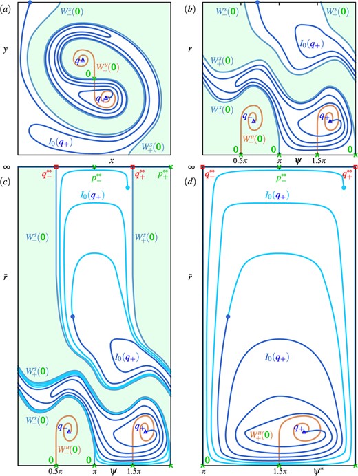
Illustration of the geometric properties of  in region A. Panel ((a)) is a sketch of the phase portrait of region A with
  in the |$(x, y)$|-plane. Panel ((b)) is its representation in the |$(\psi , r)$|-plane of polar coordinates around
  ; note that the two branches
 and
 of the stable manifold, and the two branches
  and
and  of the unstable manifold, end on the bottom line where |$r = 0$| at their respective values of the angular variable |$\psi $|. Panel (|$c$|) shows the representation in the |$(\psi , \bar {r})$|-plane of compactified polar coordinates, where
  has also been extended (cyan curve). Here, |$\bar {r}$| is the compactified radial direction, and the top horizontal line represents infinity with the equilibria
  and
and  . Panel (|$d$|) is a sketch of just the basin (
 ), where its boundary
  has been straightened out. Invariant objects are labelled as in Figure 2; compare with Figure 4.
3.3 Isochrons in region B
In region B, after the saddle-node bifurcation |$\textbf {\texttt {SNL}}$|, there are now the two additional isochron foliations |$\mathcal {I}\left (\varGamma ^{s}\right )$| and |$\mathcal {U}\left (\varGamma ^u\right )$| of the periodic orbits |$\varGamma ^{s}$| and |$\varGamma ^u$|, respectively. Figure 6 shows all isochron foliations with the phase portrait in region |$\boldsymbol {B}$| in the (rotated) |$(v, w)$|-plane. In panel (|$a$|) all three isochron foliations are shown together with the phase portrait, as in Figure 3 but magnified. The three individual foliations are shown separately with the phase portrait in panels (|$b$|)and(|$d$|). Figure 6(|$a$|) shows more clearly that the two foliations |$\mathcal {I}\left (\varGamma ^{s}\right )$| and |$\mathcal {U}\left (\varGamma ^u\right )$| intersect transversely in the annulus bounded by |$\varGamma ^{s}$| and |$\varGamma ^u$|. Note also that outside |$\varGamma ^{s}$| the foliation |$\mathcal {I}\left (\varGamma ^{s}\right )$| extends to infinity.
Isochron geometry in region B in the (rotated) |$(v, w)$|-plane, with invariant objects labelled as in Fig. 2. Panel ((a)) shows the phase portrait of region B, consisting of  and
and  and
and  , together with ten isochrons of
  and 20 isochrons each of
  and
and  . Panel (|$b$|) shows the phase portrait with only
  , panel (|$c$|) with only
  , and panel (|$d$|) with only
  ; each isochron is coloured according to its phase |$\theta $| as given by the colour bars. Along the trajectories
  (dark and light green, respectively, not shown in panel (|$b$|) the foliations
  and
and  have quadratic tangencies. Compare with Figs. 2 and 3.
More importantly, Fig. 6 illustrates the interaction of |$U_{0}(\varGamma ^u)$| with |$\mathcal {I}\left (q_{\pm }\right )$| (only isochrons in |$\mathcal {I}\left (q_{+}\right )$| are shown in Figure 6). First of all, the basins |$\mathcal {A}\left (q_{\pm }\right )$| no longer extend all the way to infinity, but they are now winding basins that accumulate onto the repelling periodic orbit |$\varGamma ^u$|. Note that their boundary |$W^s(\boldsymbol {0})$| approaches |$\varGamma ^u$| very quickly to produce an extremely narrow spiralling channel. In this channel, as in region |$\boldsymbol {A}$|, the isochrons of |$\mathcal {I}\left (q_{\pm }\right )$| feature very sharp turns, of which only the first few are visible in Figs. 6(a) and 6(d). Since these turns are very close to |$\varGamma ^u$| where |$U_{0}(\varGamma ^u)$| is almost linear, there must be quadratic tangencies between |$\mathcal {I}\left (q_{\pm }\right )$| and |$U_{0}(\varGamma ^u)$|. These occur along a symmetric pair of trajectories |$O_{\pm }$|, which spiral into |$q_{\pm }$| in forward time and accumulate onto |$\varGamma ^u$| in backward time. Notice from Figs. 6(a) and 6(c) how the isochrons of |$U_{0}(\varGamma ^u)$| develop sharp turns associated with the quadratic tangencies with |$\mathcal {I}\left (q_{+}\right )$| along |$O_{+}$|. This happens while any isochron |$U_{\theta }(\varGamma ^u) \in \mathcal {U}(\varGamma ^u)$| accumulates onto |$\overline {W^u(\boldsymbol {0})} = q_{\pm } \cup W^u(\boldsymbol {0}) \cup \boldsymbol {0}$|; hence, it must also have tangencies with the foliation |$\mathcal {I}\left (q_{-}\right )$| along |$O_{-}$| (not shown).
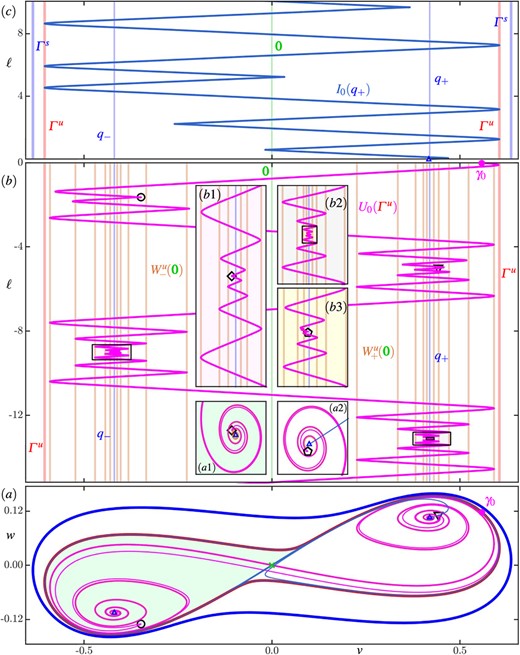
The relevant invariant objects are still very close to one another in the |$(v, w)$|-plane, which is why we illustrate these properties of |$U_{0}(\varGamma ^u)$| and |$\mathcal {I}\left (q_{+}\right )$| in Figure 7 by showing the respective zero-phase isochrons also in terms of their arclength |$\ell $|. Panel (|$a$|) shows the phase portrait of region |$\boldsymbol {B}$| in the |$(v,w)$|-plane with only |$I_{0}(q_{+})$| and |$U_{0}(\varGamma ^u)$|. Note how |$U_{0}(\varGamma ^u)$|, which starts at |$\gamma _{0} \in \varGamma ^u$|, visits both basins |$\mathcal {A}\left (q_{\pm }\right )$| while it accumulates onto the boundary |$\overline {W^u(\boldsymbol {0})}$| of its own basin |$\mathcal {R}(\varGamma ^u)$|; the first two sharp turns of |$U_{0}(\varGamma ^u)$| that ensue are marked by a circle ( ) and a triangle (
 ), respectively. The inset panels (|$a1$|)and(|$a2$|) are enlargements near |$q_{-}$| and |$q_{+}$|, respectively, that show two further sharp turns that are marked by a diamond (
 ) and a pentagon (
 ), respectively.
Details of isochron geometry of  and
and  in region B. Panel ((a)) shows the phase portrait of region |$\boldsymbol {B}$| in the |$(v,w)$|-plane with the zero-phase isochrons
  (dark blue) and
  (magenta). Panels (|$b$|)and (|$c$|) show how the |$v$|-coordinate along
  and
and  , respectively, change with arclength |$\ell $|, where the |$v$|-range is as in panel (|$a$|); here, the vertical lines indicate the positions of the equilibria
  and
and  , as well as the folds of
  with respect to the |$v$|-axis in panel (|$b$|), and the folds in |$v$| of the periodic orbits
  and
and  . The black circle (
 ), triangle (
 ), diamond (
 ), and pentagon (
 ) in panels (|$a$|)and(|$b$|) mark the first four sharp turns of
  , respectively; the insets are enlargements near
  in panel (a) and of correspondingly shaded areas in panel (|$b$|). Compare with Figure 6.
Figure 7(b) shows the (signed) arclength |$\ell $| of |$U_{0}(\varGamma ^u)$| against its |$v$|-coordinate, together with vertical lines that indicate the positions on the |$v$|-axis of the equilibria |$q_{\pm }$| and |$\boldsymbol {0}$| and the folds of the two branches |$W^u_{+}(\boldsymbol {0})$| and |$W^u_{-}(\boldsymbol {0})$| of the unstable manifold |$W^u(\boldsymbol {0})$| with respect to |$v$|. This panel better illustrates how |$U_{0}(\varGamma ^u)$| moves from left to right and spirals ever closer into |$q_{-}$| and |$q_{+}$| while accumulating onto |$\overline {W^u(\boldsymbol {0})}$|; note that its arclength is negative, because we are considering the branch of |$U_{0}(\varGamma ^u)$| that lies inside |$\varGamma ^u$|. In Fig. 7(b) we observe that |$U_{0}(\varGamma ^u)$| moves away from |$\gamma _{0}$| (pink dot) by following the unstable manifold |$W^u(\boldsymbol {0})$| (initially along the branch |$W^s_{+}(\boldsymbol {0})$| towards, and then well past |$\boldsymbol {0}$|; in the process, |$U_{0}(\varGamma ^u)$| has two folds (with respect to |$v$|) near the folds of |$W^u_{\pm }(\boldsymbol {0})$|. However, the third fold, marked by the circle () near |$q_{-}$|, is not near a fold of |$W^u(\boldsymbol {0})$|. Hence, this fold is the first sharp turn of |$U_{0}(\varGamma ^u)$| where it switches direction to follow (the other side of) |$W^u(\boldsymbol {0})$| (along the same branch |$W^u_{-}(\boldsymbol {0})$| of |$W^u(\boldsymbol {0})$| back towards and well past |$\boldsymbol {0}$|. After passing the origin, |$U_{0}(\varGamma ^u)$| has quite a number of folds near the folds of |$W^u(\boldsymbol {0})$|, until there is a second sharp turn near |$q_{+}$|, marked by the triangle (). The process repeats and we find a third sharp turn () nearer |$q_{-}$| and a fourth sharp turn () nearer |$q_{+}$|; they are illustrated in the enlargement panel (|$b1$|) and the successive enlargement panels (|$b2$|)and(|$b3$|), respectively. Note that successive sharp turns of |$U_{0}(\varGamma ^u)$| occur deeper and deeper into the spirals formed by the branches of |$W^u(\boldsymbol {0})$|; this feature is represented in panel (|$b$|) as an increasing number of folds of |$W^u(\boldsymbol {0})$| before and after successive sharp turns.
Similarly, Fig. 7((c)) illustrates how |$I_{0}(q_{+})$| accumulates onto the boundary |$W^s(\boldsymbol {0})$| of its basin |$\mathcal {A}\left (q_{+}\right )$|; this involves following the stable manifold |$W^s(\boldsymbol {0})$| for exceedingly longer periods of time, with sharp turns in between where |$I_{0}(q_{+})$| switches over from one branch of |$W^s(\boldsymbol {0})$| to the other, specifically, from |$W^s_{-}(\boldsymbol {0})$| to |$W^s_{+}(\boldsymbol {0})$|. The situation is very similar to that in region |$\boldsymbol {A}$| in Fig. 4(c), but now |$\mathcal {A}\left (q_{+}\right )$| is a winding basin that accumulates onto |$\varGamma ^u$|.
We again represent these insights as topological sketches to bring out the observed isochron geometry more clearly. Figures 8(a1) and 8(b1) show the zero-phase isochrons |$U_{0}(\varGamma ^u)$| and |$I_{0}(q_{+})$|, respectively, inside the periodic orbit |$\varGamma ^u$| in both Cartesian and polar coordinates. These sketches stress qualitative features of the geometry; in particular, the narrow channels of the basins |$\mathcal {A}\left (q_{\pm }\right )$| that are hardly visible in Fig. 7(|$a$|) are shown much wider so that the respective accumulation processes of the isochrons can readily be sketched.
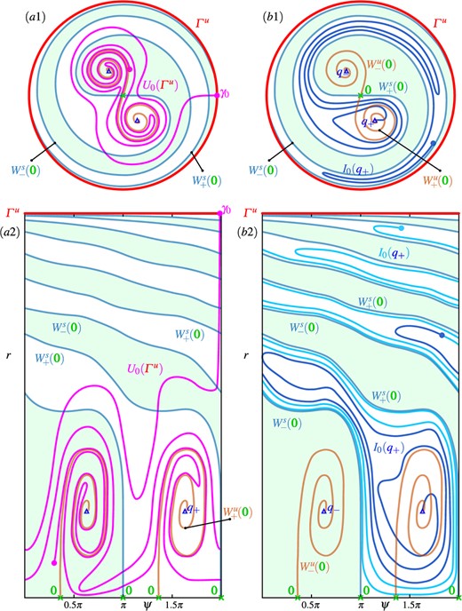
Illustrations of the geometric properties in region B of  in panels (a1) and (a2) and of
  in panels (b1) and (b2). Panels (a1) and (b1) are sketches of the phase portrait of region B inside the repelling periodic orbit
  in the |$(x, y)$|-plane with
  and
and  , respectively. Panels (a2) and (b2) show the same objects in the |$(\psi , r)$|-plane of polar coordinates around
  ; here,
  has been extended (cyan curve), and the red horizontal line at the top of the panel represents , onto which the winding basins (
 ) accumulate. Invariant objects are labelled as in Figure 2; compare with Figs. 6 and 7.
Figure 8(a1) is a sketch in the |$(x, y)$|-plane of |$U_{0}(\varGamma ^u)$| inside the repelling periodic orbit |$\varGamma ^u$|. The isochron |$U_{0}(\varGamma ^u)$| starts at the zero-phase point |$\gamma _{0} \in \varGamma ^u$| and then enters the inside of |$\varGamma ^u$| to accumulate onto the basin boundary |$\overline {W^u(\boldsymbol {0})}$| of its basin |$\mathcal {A}\left ({\varGamma _u}\right )$| in a spiralling fashion. The polar-coordinate representation in panel (|$a2$|) shows more clearly how |$U_{0}(\varGamma ^u)$| has alternating episodes in the two basins |$\mathcal {A}\left (q_{\pm }\right )$| as it approaches simultaneously the two branches |$W^u_{-}(\boldsymbol {0})$| and |$W^u_{+}(\boldsymbol {0})$| of the unstable manifold |$W^u(\boldsymbol {0})$|. As a consequence, each of the successive sharp turns of |$U_{0}(q_{+})$| lies deeper in the spiral of |$W^u_{-}(\boldsymbol {0})$| and |$W^u_{+}(\boldsymbol {0})$| and, hence, closer to |$q_{-}$| and to |$q_{+}$|, respectively.
Figure 8(b1) is a sketch in the |$(x, y)$|-plane of |$I_{0}(q_{+})$| in the interior of its winding basin |$\mathcal {A}\left (q_{+}\right )$| inside |$\varGamma ^u$|. The isochron |$I_{0}(q_{+})$| is shown spiralling outward to accumulate onto the manifold |$W^s(\boldsymbol {0}) \subset \partial \mathcal {A}\left (q_{+}\right )$|, which in turn accumulates quickly onto |$\varGamma ^u \subset \partial \mathcal {A}\left (q_{+}\right )$|. This is illustrated further in panel (|$b2$|) in the polar-coordinate representation, where |$I_{0}(q_{+})$| has been extended further to show the accumulation process. While spiralling out from |$q_{+}$|, the isochron |$I_{0}(q_{+})$| makes further and further excursions into the increasingly narrower channel formed by |$\mathcal {A}\left (q_{+}\right )$| as it accumulates onto |$\varGamma ^u$|. Up to some finite arclength, the curve |$I_{0}(q_{+})$| from |$q_{+}$| in |$\mathcal {A}\left (q_{+}\right )$| has a finite number of spiral loops, which is illustrated in Fig. 8(b2). The difference with region |$\boldsymbol {A}$| is that in region |$\boldsymbol {B}$|, there is an infinite amount of winding of the basin |$\mathcal {A}\left (q_{+}\right )$|, rather than only a finite number of rotations. Therefore, it is not possible to transform the entire (infinitely) winding basin |$\mathcal {A}\left (q_{+}\right )$| diffeomorphically to a simple box as in Fig. 5(d) (as this would then not involve the accumulation of |$\mathcal {A}\left (q_{+}\right )$| on a topological circle). Indeed, the fact that there is now a winding basin leads to infinitely many sharp turns and associated tangencies of |$\mathcal {I}\left (q_{+}\right )$| (and also of |$\mathcal {I}\left (q_{-}\right )$| by symmetry) with |$U_{0}(\varGamma ^u)$|; compare Fig. 5(d) and Fig. 8(b2).
Since |$U_{0}(\varGamma ^u)$| and |$I_{0}(q_{+})$| are representative isochrons, their respective geometric properties are shared with the respective foliations. The isochrons of |$U_{0}(\varGamma ^u)$| and of |$\mathcal {I}\left (q_{\pm }\right )$| both accumulate onto a spiralling basin boundary, namely |$\overline {W^u(\boldsymbol {0})}$| and |$\overline {W^s(\boldsymbol {0})}$|, respectively. This explains the existence of quadratic tangencies between the two foliations along two (symmetrically related) orbits |$O_{\pm }$| in the respective spiralling basins |$\mathcal {A}\left (q_{\pm }\right )$|.
3.4 Isochrons in region C
In region C, after the homoclinic bifurcation |$\textbf {\texttt {HOM}}$|, the invariant manifolds |$W^s(\boldsymbol {0})$| and |$W^u(\boldsymbol {0})$| have changed their relative positions. Hence, there is now the symmetric pair of repelling periodic orbits |$\varGamma ^u_{\pm }$| (instead of |$\varGamma ^u$|) with backward-time isochron foliations |$\mathcal {U}(\varGamma ^u_{\pm })$| in their basins |$\mathcal {R}(\varGamma ^u_{\pm })$|. Figure 9 shows all isochron foliations with the phase portrait in region |$\boldsymbol {C}$| in the (rotated) |$(v, w)$|-plane. In panel (|$a$|) all three isochron foliations are shown together with the phase portrait, as in Figure 3, while panels (|$b$|)and(|$d$|) show the three individual foliations. Note that, since |$W^u(\boldsymbol {0})$| accumulates onto |$\varGamma ^{s}$|, the two basins |$\mathcal {R}(\varGamma ^u_{\pm })$| bounded by the |$q_{\pm }$|, |$W^u(\boldsymbol {0})$| and |$\varGamma ^{s}$|, are winding basins and, in fact, winding annuli because the isolated points |$q_{\pm }$| are in their boundary. The basins |$\mathcal {A}\left (q_{\pm }\right )$|, on the other hand, are bounded by the respective periodic orbits |$\varGamma ^u_{\pm }$| and, hence, are no longer winding.
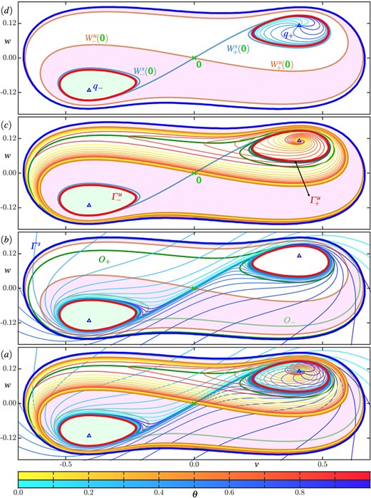
Isochron geometry in region C in the (rotated) |$(v, w)$|-plane, with invariant objects labelled as in Fig. 2. Panel ((a)) shows the phase portrait of region C, consisting of  and
and  and
and  , together with ten isochrons each of
  and
and  and 20 isochrons of
  . Panel (|$b$|) shows the phase portrait with only
  , panel (|$c$|) with only
  , and panel (|$d$|) with only
  ; each isochron is coloured according to its phase |$\theta $| as given by the colour bars. Along the trajectories
  (dark and light green, respectively, absent from panel (|$a$|)) the foliations
  and
and  have quadratic tangencies. Compare with Figs. 2 and 3.
As panels ((a),(c)) and ((d)) of Figure 9 illustrate, in region C, the foliations |$\mathcal {I}\left (q_{+}\right )$| and |$\mathcal {U}(\varGamma ^u_{+})$| intersect transversely in |$\mathcal {A}\left (q_{+}\right ) \cup \mathcal {R}(\varGamma ^{u}_{+})$|; due to symmetry, the same is true for |$\mathcal {I}\left (q_{-}\right )$| and |$\mathcal {U}(\varGamma ^u_{-})$| (not shown). In contrast, there are now quadratic tangencies between |$\mathcal {I}\left (\varGamma ^{s}\right )$| and |$\mathcal {U}(\varGamma ^u_{+})$| along the orbit |$O_{+} \subset \mathcal {R}(\varGamma ^u_{+})$| and, similarly, with |$\mathcal {U}(\varGamma ^u_{-})$| (not shown) along |$O_{-} \subset \mathcal {R}(\varGamma ^u_{-})$|. In a local neighbourhood of |$\varGamma ^{u}_{+}$| where |$\mathcal {U}(\varGamma ^u_{+})$| is almost linear they lead to sharp folds of |$\mathcal {I}\left (\varGamma ^{s}\right )$|, while near |$\varGamma ^{s}$| where |$\mathcal {U}(\varGamma ^s)$| is almost linear they lead to sharp folds of |$\mathcal {U}(\varGamma ^u_{+})$|; see panels (|$b$|)and(|$c$|).
The isochrons in |$\mathcal {I}\left (\varGamma ^{s}\right )$| and |$\mathcal {U}(\varGamma ^{u}_{+})$| accumulate rapidly onto |$W^s(\boldsymbol {0})$| and |$W^u(\boldsymbol {0})$|, which in turn accumulate rapidly onto the periodic orbits |$\varGamma ^{u}_{+}$| and |$\varGamma ^{s}$|, respectively. Therefore, the details of the geometry of these isochrons is somewhat obscured in Figure 9. To illustrate their properties we present in Figure 10 only the respective zero-phase isochrons along with their arclength plots. Panel (|$a$|) shows the phase portrait in the |$(v, w)$|-plane of region |$\boldsymbol {C}$| with |$\mathcal {I}_0(\varGamma ^{s})$| and |$\mathcal {U}_0(\varGamma ^{u}_{+})$|. Starting from |$\gamma _{0}$| (blue dot) we see that |$\mathcal {I}_0(\varGamma ^{s})$| quickly approaches |$W^s(\boldsymbol {0})$| and follows this manifold past |$\boldsymbol {0}$| before switching over to the other side of |$W^s(\boldsymbol {0})$| at a first fold point near |$\varGamma ^u_-$|. This can only really be seen in Fig. 10(b) where the |$v$|-coordinate of isochron |$\mathcal {I}_0(\varGamma ^{s})$| is shown over the same range as in panel (|$a$|) against its arclength |$\ell $| on the vertical axis. Here, folds with respect to the |$v$|-direction of |$\varGamma ^u_{\pm }$| and the branches of |$W^s(\boldsymbol {0})$|, as well as the positions of the equilibria |$q_{\pm }$| and |$\boldsymbol {0}$|, are indicated by vertical lines in the panel. Note that, because we are considering the branch of |$\mathcal {I}_0(\varGamma ^{s})$| inside |$\varGamma ^{s}$|, its arclength |$\ell $| is negative.
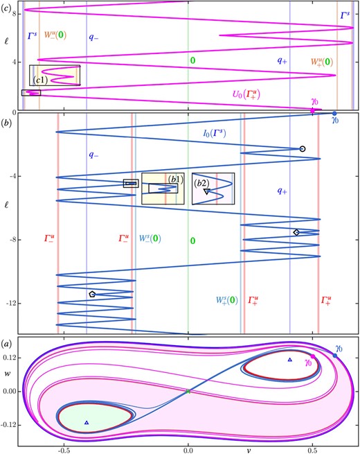
Details of isochron geometry of  and
and  in region C. Panel ((a)) shows the phase portrait of region |$\boldsymbol {C}$| in the |$(v,w)$|-plane with the zero-phase isochrons
  (dark blue) and
  (magenta). Panels (b) and (c) show how the |$v$|-coordinate along
  and
and  , respectively, change with arclength |$\ell $|, where the |$v$|-range is as in panel (|$a$|); here, the vertical lines indicate the positions of the equilibria
  and
and  , as well as the folds of
  and
and  with respect to the |$v$|-axis in panels (|$b$|)and(|$c$|), respectively, and the folds in |$v$| of the periodic orbits
  and
and  . The black circle (
 ), triangle (
 ), diamond (
 ), and pentagon (
 ) in panel (|$b$|) mark the first four sharp turns of
  , respectively; the insets are enlargements of correspondingly shaded areas in panel (|$b$|). Compare with Figure 9.
The first sharp turn near |$\varGamma ^u_-$| that occurs away from the folds of |$\varGamma ^{u}_{+}$| and |$W^s_{+}(\boldsymbol {0})$|, is marked by a black circle (). Subsequently, the curve |$\mathcal {I}_0(\varGamma ^{s})$| follows |$W^s(\boldsymbol {0})$| past |$\boldsymbol {0}$| to approach |$\varGamma ^{u}_{+}$| where it has its second sharp fold that is now further down the spiral of |$W^s(\boldsymbol {0})$|. Identifying it requires two successive enlargements, shown in panels (|$b1$|)and(|$b2$|) of Figure 9(|$b$|), where the second fold is marked by a black triangle (). The process then repeats, with alternating visits of |$W^s(\boldsymbol {0})$| for increasing arclength to neighborhoods of |$\varGamma ^u_{\pm }$|, owing to the fact that |$\mathcal {I}_0(\varGamma ^{s})$| exists in both basins of repulsion |$\mathcal {R}(\varGamma ^u_{\pm })$|. This yields the two further sharp folds marked by the diamond () and the pentagon () in Figure 9(|$b$|). Note that successive sharp turns occur deeper along the spirals formed by the two branches of |$W^s(\boldsymbol {0})$|; the number of other folds before each sharp turn indicates how deep down the sharp turn occurs in this spiral.
Figure 10(c) shows the accumulation of |$\mathcal {U}_0(\varGamma ^{u}_{+})$| onto the boundary |$\overline {W^u(\boldsymbol {0})}$| of the winding basin |$\mathcal {R}(\varGamma ^{u}_{+})$| outside of |$\varGamma ^{u}_{+}$|. For increasing arclength |$\ell $| the isochron extends from |$\gamma _{0}$| (pink dot) until making its first sharp turn to the left of |$\varGamma ^u_-$|; this is clearly visible in panel (|$a$|) but requires the enlargement panel (|$c1$|) to be identified as a fold with respect to the |$v$|-direction in panel (|$c$|). Note that before this sharp turn, |$\mathcal {U}_0(\varGamma ^{u}_{+})$| remains relatively far away from |$\partial \mathcal {R}(\varGamma ^{u}_{+}) = \overline {W^u(\boldsymbol {0})}$|. As |$\ell $| increases further, the isochron |$\mathcal {U}_0(\varGamma ^{u}_{+})$| now follows |$W^u_{-}(\boldsymbol {0})$| closely back around |$\varGamma ^{u}_{+}$|, past |$\boldsymbol {0}$|, past |$\varGamma ^u_-$| and past |$\varGamma ^{u}_{+}$| once more, before making its second sharp turn; this very sharp turn cannot be seen in panel (|$a$|) but can be identified in panel (|$c$|) as occurring near |$v \approx 0.1$|. The isochron |$\mathcal {U}_0(\varGamma ^{u}_{+})$| then follows |$W^u_{-}(\boldsymbol {0})$| closely, back past |$\boldsymbol {0}$| and the process repeats with increasingly sharper turns as |$W^u(\boldsymbol {0})$| accumulates onto |$\varGamma ^{s}$|.
Figure 11 presents topological sketches that illustrate the observed isochron geometry. Panels and show the zero-phase isochrons |$\mathcal {I}_0(\varGamma ^{s})$| and |$\mathcal {U}_0(\varGamma ^{u}_{+})$|, respectively, in Cartesian coordinates inside the periodic orbit |$\varGamma ^{s}$|, while panels (|$a2$|)and(|$b2$|) show them in polar coordinates. Again, these sketches stress qualitative features; specifically, the zero-phase isochrons are shown as accumulating less rapidly onto their basin boundaries, so that the respective accumulation processes of the isochrons can readily be illustrated.
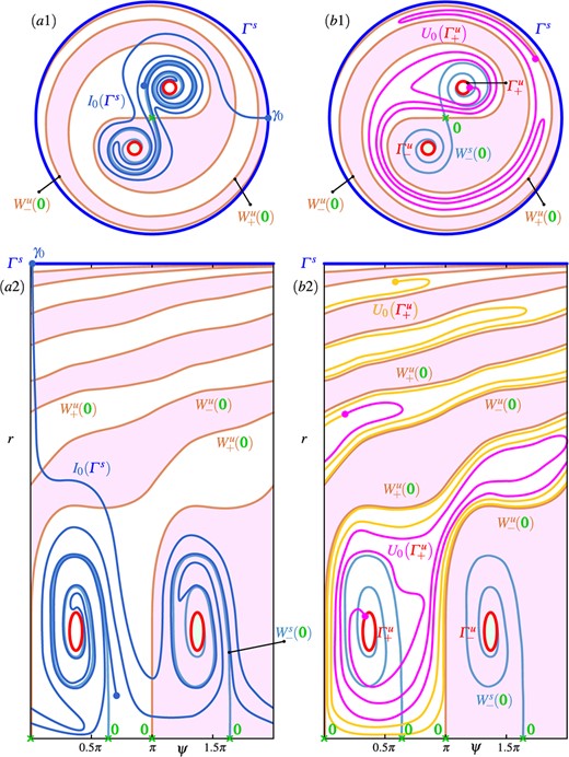
Illustrations of the geometric properties in region C of  in panels (a1) and (a2) and of
  in panels (b1) and (b2). Panels (a1) and (b1) are sketches of the phase portrait of region C inside the attracting periodic orbit
  in the |$(x, y)$|-plane with
  and
and  , respectively. Panels (a2) and (b2) show the same objects in the |$(\psi , r)$|-plane of polar coordinates around
  ; here, the blue horizontal line at the top of the panel represents
  , onto which the winding basins
  accumulate, and
  has also been extended (yellow curve). Invariant objects are labelled as in Figure 2; compare with Figs. 9 and 10.
In panel ((a1)), the isochron |$\mathcal {I}_0(\varGamma ^{s})$| starts at the zero-phase point |$\gamma _{0}$| (blue dot) and begins to accumulate onto the basin boundary |$\overline {W^s(\boldsymbol {0})}$| of its basin |$\mathcal {A}\left ({\varGamma ^{s}}\right )$| by spiralling around it. The polar-coordinate representation in panel (|$a2$|) shows more clearly how |$\mathcal {I}_0(\varGamma ^{s})$| moves between the two basins |$\mathcal {R}(\varGamma ^u_{\pm })$| as it approaches the two branches |$W^s_{-}(\boldsymbol {0})$| and |$W^s_{+}(\boldsymbol {0})$| of the stable manifold |$W^s(\boldsymbol {0})$|. As a consequence, each of the successive sharp turns of |$\mathcal {I}_0(\varGamma ^{s})$| lies deeper into the spirals of |$W^s_{-}(\boldsymbol {0})$| and |$W^s_{+}(\boldsymbol {0})$| and, hence, closer to |$\varGamma ^u_-$| and to |$\varGamma ^{u}_{+}$|, respectively.
The sketch in Cartesian coordinates in Fig. 11((b1)) shows the branch of the isochron |$\mathcal {U}_0(\varGamma ^{u}_{+})$| inside its winding basin |$\mathcal {R}(\varGamma ^{u}_{+})$| that lies outside |$\varGamma ^u$|. Notice how |$\mathcal {U}_0(\varGamma ^{u}_{+})$| spirals outward to accumulate on the basin boundary |$W^u(\boldsymbol {0})$|, which in turn accumulates on |$\varGamma ^{s}$|. The polar-coordinate representation in panel ((b2)) also shows an extension of |$\mathcal {U}_0(\varGamma ^{u}_{+})$| (yellow curve) to show more of the accumulation process. The sharp turns of |$\mathcal {U}_0(\varGamma ^{u}_{+})$| occur further and further along the channel of |$\mathcal {A}\left ({\varGamma ^+_u}\right )$| as it accumulates onto |$\varGamma ^{s}$|, with |$\mathcal {U}_0(\varGamma ^{u}_{+})$| following along the branches of |$W^u(\boldsymbol {0})$| more closely with each fold.
Comparison between the sketches presented in Figs. 8 and 11 shows that the foliations |$U_{0}(\varGamma ^u)$| inside of |$\varGamma ^u$| in region |$\boldsymbol {B}$| and |$\mathcal {I}_0(\varGamma ^{s})$| inside of |$\varGamma ^{s}$| in region |$\boldsymbol {C}$|, respectively, are topologically the same as families of curves (that is, not taking into account the direction of time); namely they share the key property that they both accumulate onto a spiralling curve in the respective basin boundary given by the closure of an (un)stable manifold. Similarly, the foliations |$\mathcal {U}_0(\varGamma ^{u}_{+})$| inside |$\mathcal {A}\left ({\varGamma ^{s}}\right ) \cap \mathcal {R}(\varGamma ^{u}_{+})$| in region |$\boldsymbol {B}$| and |$\mathcal {I}_0(\varGamma ^{s})$| inside of |$\varGamma ^{s}$| in region |$\boldsymbol {C}$|, respectively, share the topological property of spiralling onto the boundary of a winding basin formed by the closure of an (un)stable manifold that contains a circle, which implies the existence of tangencies between the isochron foliation in the winding basin and that of the periodic orbit on which it accumulates. Overall, we conclude that the homoclinic bifurcation |$\textbf {\texttt {HOM}}$| induces a rather dramatic exchange between the geometric properties of isochron foliations in basins of attraction and those in basins of repulsion.
3.5 Isochrons in region D
In region D, after the (subcritical) Hopf bifurcation |$\textbf {\texttt {HB}}$|, the repelling periodic orbits |$\varGamma ^u_{\pm }$| have disappeared and the focus equilibria |$q_{\pm }$| are now repelling. With the basin of attraction of |$q_{\pm }$|, also the foliations |$\mathcal {I}\left (q_{\pm }\right )$| have disappeared. Instead the points |$q_{\pm }$| now have basins of repulsion |$\mathcal {R}(q_{\pm })$|, which are winding basins because the boundary |$W^u(\boldsymbol {0})$| between them still accumulates on the attracting periodic orbit |$\varGamma ^s$|.
Figure 12 shows the different invariant objects and foliations in the (rotated) |$(v, w)$|-plane; shown are in panel ((a)), the interactions of twenty and ten isochrons of the foliations |$\mathcal {I}\left (\varGamma ^{s}\right )$| and |$\mathcal {U}(q_{+})$|, respectively, which are shown separately in panels (|$b$|)and(|$c$|). The foliation |$\mathcal {I}\left (\varGamma ^{s}\right )$| of |$\mathcal {A}\left ({\varGamma ^{s}}\right )$| inside |$\varGamma ^{s}$| still accumulates on its boundary |$\overline {W^s(\boldsymbol {0})}$| but now |$\overline {W^s(\boldsymbol {0})} = q_{-} \cup q_{+} \cup W^s(\boldsymbol {0})$|. Moreover, |$\mathcal {U}(q_{+})$| foliates the winding basin |$\mathcal {R}(q_{+})$| and it is tangent to |$\mathcal {I}\left (\varGamma ^{s}\right )$| along the trajectory |$O_{+}$|. Comparison between Fig. 12(|$a$|) and Fig. 9(|$a$|) shows that in the transition through the Hopf bifurcation |$\textbf {\texttt {HB}}$| the basins |$\mathcal {R}(q_{\pm })$| and the foliations |$\mathcal {U}(q_{\pm })$| in region |$\boldsymbol {D}$| are the continuations of |$\mathcal {R}(\varGamma ^u_{\pm })$| and |$\mathcal {U}(\varGamma ^u_{\pm })$| (outside of |$\varGamma ^u_{\pm }$|) in region |$\boldsymbol {C}$|. This is in agreement with the observation by Langfield et al. (2015) that foliations can be continued through a Hopf bifurcation; however, we have here a situation with a single trajectory |$O_{+}$| within |$\mathcal {R}(q_{+})$| along which one finds quadratic tangencies of two foliations, while in (Langfield et al., 2015) there is a pair of such tangency orbits (generated in a CIFT; see Section 1.4). Nevertheless, we also find that the tangency orbits |$O_{+}$| and its symmetric counterpart |$O_{-}$| in |$\mathcal {R}(q_{-})$| can be continued as continuous objects through |$\textbf {\texttt {HB}}$| during the transition from region |$\boldsymbol {C}$| to region |$\boldsymbol {D}$|.
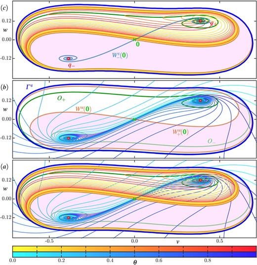
Isochron geometry in region D in the (rotated) |$(v, w)$|-plane, with invariant objects labelled as in Fig. 2. Panel ((a)) shows the phase portrait of region D, consisting of  and
and  , and
, and  , together with ten isochrons of
  and 20 isochrons of
  . Panel (|$b$|) shows the phase portrait with only
  , and panel (|$c$|) with only
  ; each isochron is coloured according to its phase |$\theta $| as given by the colour bars. Along the trajectories
  (dark and light green, respectively) the foliations
  and
and  have quadratic tangencies. Compare with Figs. 2 and 3.
In other words, the foliations |$\mathcal {U}(q_{\pm })$| of the winding basins in region D inherit the geometric properties of the foliation |$\mathcal {U}(\varGamma ^u_{\pm })$| of the winding basins in region |$\boldsymbol {C}$| (outside of |$\varGamma ^u_{\pm }$|); the difference is that the curve |$W^s(\boldsymbol {0})$| in the boundary of |$\mathcal {A}\left ({\varGamma ^{s}}\right )$| accumulates in region |$\boldsymbol {D}$| on the points |$q_{\pm }$|, while in region |$\boldsymbol {C}$| is accumulates on a pair of circles (the repelling periodic orbits |$\varGamma ^u_{\pm }$|). This is illustrated further in Figure 13. Panel (|$a$|) shows the phase portrait in region |$\boldsymbol {D}$| in the (rotated) |$(v, w)$|-coordinates with |$\mathcal {I}_0(\varGamma ^{s})$| (dark blue) and |$U_0(q_{+})$| (magenta), and panels (|$a1$|)and(|$a2$|) are enlargements near |$q_{-}$| and |$q_{+}$|, respectively. The two zero-phase isochrons of |$\mathcal {I}_0(\varGamma ^{s})\in \mathcal {I}\left (\varGamma ^{s}\right )$| and |$U_0(q_{+}) \in \mathcal {U}(q_{+})$| are shown in panels (|$b$|)and(|$c$|) in terms of their arclength |$\ell $| against the |$v$|-coordinate; here, the |$v$|-range is as in Fig. 13(|$a$|) and vertical lines indicate the equilibria |$q_{\pm }$| (red) and |$\boldsymbol {0}$| (green) and the folds of the branches of |$W^s(\boldsymbol {0})$| (blue).
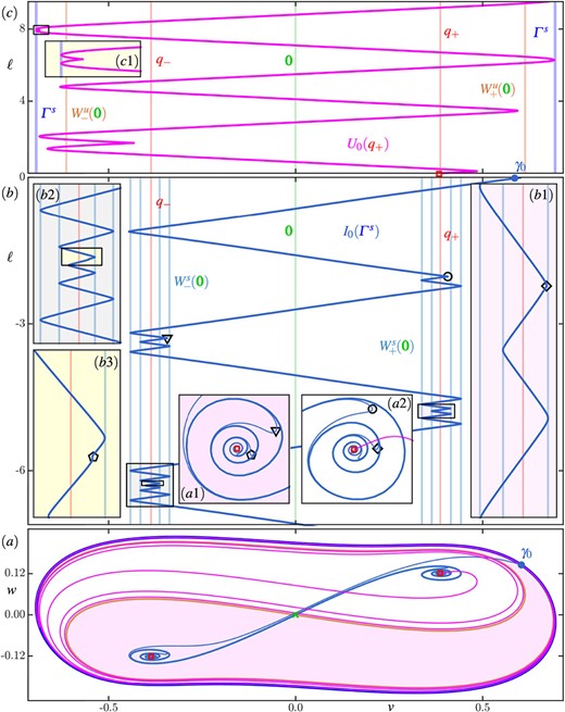
Details of isochron geometry of  and
and  in region D. Panel ((a)) shows the phase portrait of region |$\boldsymbol {D}$| in the |$(v,w)$|-plane with the zero-phase isochrons
  (dark blue) and
  (magenta). Panels (b) and (c) show how the |$v$|-coordinate along
  and
and  , respectively, change with arclength |$\ell $|, where the |$v$|-range is as in panel (|$a$|); here, the vertical lines indicate the positions of the equilibria
  and
and  , as well as the folds of
  and
and  with respect to the |$v$|-axis in panels (|$b$|)and(|$c$|), respectively, and the folds in |$v$| of the periodic orbit
  . The black circle (
 ), triangle (
 ), diamond (
 ) and pentagon (
 ) in panel (|$b$|) mark the first four sharp turns of
  , respectively; the insets are enlargements of correspondingly shaded areas in panels (|$a$|)and(|$b$|). Compare with Figure 12.
For increasing |$\ell $|, the curve |$\mathcal {I}_0(\varGamma ^{s})$| moves between neighbourhoods of |$q_{-}$| and |$q_{+}$|; it has its first sharp fold near |$q_{+}$|, marked by the black circle ( ), and subsequent sharp turns alternatingly near |$q_{-}$| and |$q_{+}$| at the black triangle (
 ), diamond (
 ) and pentagon (
 ), respectively; see Fig. 13(b) and the enlargements in panels (|$a1$|),(|$a2$|)and (|$b1$|)–(|$b3$|). Note that these sharp folds, which are clearly identified in the phase portrait, now occur quite close to folds of |$W^s(\boldsymbol {0})$| in |$v$|. As we have come to expect, |$\mathcal {I}_0(\varGamma ^{s})$| switches from one side to the other side of |$W^s(\boldsymbol {0})$| at each of the marked sharp turns; compare with Fig. 10(b).
As Fig. 13((c)) shows, the curve |$U_0(q_{+})$| has its first sharp turn for |$\ell \approx 2$| where |$U_0(q_{+})$| switches from following |$W^u_{-}(\boldsymbol{0})$| after its first (close) pass of |$boldsymbol{0}$| to following the branch |$W^u_{+}(\boldsymbol {0})$| of |$W^u(\boldsymbol {0})$| again. For increasing |$\ell $|, the curve |$U_0(q_{+})$| follows along |$W^u_{+}(\boldsymbol {0})$|, switching to following |$W^u_{-}(\boldsymbol {0})$| as it passes |$\boldsymbol {0}$| more closely until its second sharp turn, which is highlighted in panel (|$c1$|). Here, |$U_0(q_{+})$| switches to following |$W^u_{+}(\boldsymbol {0})$| back to near |$\boldsymbol {0}$|, and this process of switching repeats. Comparison with Fig. 10(c) shows that |$U_0(q_{+})$| in region |$\boldsymbol {D}$| has, indeed, the same geometric properties as |$\mathcal {U}_0(\varGamma ^{u}_{+})$| in region |$\boldsymbol {C}$|.
The above insights regarding the geometry of the foliations |$\mathcal {I}_0(\varGamma ^{s})$| and |$U_0(q_{+})$| are represented in sketched form also by Fig. 11, when one imagines that the repelling periodic orbits |$\varGamma ^u_{\pm }$| are contracted to the two repelling points |$q_{\pm }$|. In other words, the foliation |$\mathcal {I}\left (\varGamma ^{s}\right )$| effectively preserves its geometric properties in regions |$\boldsymbol {C}$| and |$\boldsymbol {D}$|, while |$\mathcal {U}(q_{\pm })$| is the continuation of |$\mathcal {U}(\varGamma ^u_{\pm })$| (outside of |$\varGamma ^u_{\pm }$|) from region |$\boldsymbol {C}$| to region |$\boldsymbol {D}$| as the foliation by backward-time isochrons in the pair of winding basins.
3.6 Isochrons in regions E and F
In region E, after the transition through the curve |$(\textbf {\texttt {CC}})$|, the eigenvalues of |$q_{\pm }$| are real; hence, there is no longer any spiralling associated with these equilibria and their isochron foliations |$\mathcal {U}(q_{\pm })$| have disappeared. This leaves |$\mathcal {I}\left (\varGamma ^{s}\right )$| as the only isochron foliation and it is illustrated in Figure 14 in three different ways. Shown is the phase portrait of region |$\boldsymbol {E}$| in the (rotated) |$(v, w)$|-plane with twenty phase-uniform isochrons of |$\mathcal {I}\left (\varGamma ^{s}\right )$| in panel (|$a$|) and with only the zero-phase isochron |$\mathcal {I}_0(\varGamma ^{s})$| (dark blue) in panel (|$b$|); the arclength |$\ell $| along |$\mathcal {I}_0(\varGamma ^{s})$| is plotted against its |$v$|-coordinate in panel (|$c$|). The isochrons of |$\mathcal {I}\left (\varGamma ^{s}\right )$| still accumulate onto |$\overline {W^s(\boldsymbol {0})} = q_{-} \cup q_{+} \cup W^s(\boldsymbol {0})$| in a spiralling fashion. While this is not immediately obvious from the phase portraits in panels (|$a$|)and(|$b$|), the arclength plot of |$\mathcal {I}_0(\varGamma ^{s})$| in panel (|$c$|) shows that this isochron indeed spirals around the curve |$\overline {W^s(\boldsymbol {0})}$| that connects the two equilibria |$q_{-}$| and |$q_{+}$|. This must indeed be the case because both branches of |$W^u(\boldsymbol {0})$| accumulate on |$\varGamma ^{s}$| and so intersect |$\mathcal {I}_0(\varGamma ^{s})$| near |$\varGamma ^{s}$| infinitely many times. These intersections repeat at every integer multiple of the period |$\mathrm {T}_{\varGamma ^{s}}$| of |$\varGamma ^{s}$| by the definition of asymptotic phase (1.4), meaning that |$\mathcal {I}_0(\varGamma ^{s})$| is required to intersect each branch of |$W^u(\boldsymbol {0})$|, alternatingly and infinitely many times. Hence, |$\mathcal {I}_0(\varGamma ^{s})$| spirals around |$\overline {W^s(\boldsymbol {0})}$| and its strong contraction towards |$W^s(\boldsymbol {0})$| is governed by the unstable eigenvalue of |$\boldsymbol {0}$|.
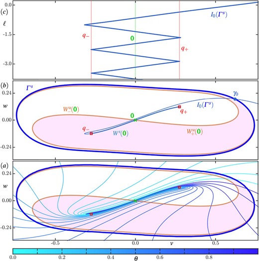
Details of isochron geometry in region E in the (rotated) |$(v, w)$|-plane. Panel ((a)) shows the phase portrait, consisting of  and
and  and
and  , and
, and  , together with ten isochrons of
  , and panel (|$b$|) shows the phase portrait with only the zero-phase isochron
  ; here, each isochron in panel (|$a$|) is coloured according to its phase |$\theta $| as given by the colour bar. Panel (|$c$|) shows how the |$v$|-coordinate along
  changes with arclength |$\ell $|, where the |$v$|-range is as in panels (|$a$|)and(|$b$|) and the vertical lines indicate the positions
  , |$\boldsymbol {0}$| and the folds of
  with respect to the |$v$|-direction. Compare with Figs. 2 and 3.
In region F, after the pitchfork bifurcation |$\textbf {\texttt {PF}}$|, the repellors |$q_{\pm }$| and their basins have disappeared and |$\boldsymbol {0}$| is now repelling. Hence, |$\boldsymbol {0}$| is the only point in the boundary of |$\mathcal {A}\left ({\varGamma ^{s}}\right )$| and the isochrons of |$\mathcal {I}\left (\varGamma ^{s}\right )$| accumulate on this point. This is illustrated in Figure 15, where panels (|$a$|)and(|$b$|) show twenty phase-uniform isochrons of |$\mathcal {I}\left (\varGamma ^{s}\right )$| and only |$\mathcal {I}_0(\varGamma ^{s})$| (dark blue) in the (rotated) |$(v, w)$|-plane, respectively; also shown here is the strong unstable manifold |$W^{uu}(\boldsymbol {0})$| of |$\boldsymbol {0}$|, which is the continuation of |$W^u(\boldsymbol {0})$| in region |$\boldsymbol {E}$| past |$\textbf {\texttt {PF}}$| into region |$\boldsymbol {F}$|. Panel (|$c$|) shows the arclength |$\ell $| along |$\mathcal {I}_0(\varGamma ^{s})$| against its |$v$|-coordinate. In region |$\boldsymbol {F}$| the isochrons of |$\mathcal {I}\left (\varGamma ^{s}\right )$| converge (as curves) to the point |$\boldsymbol {0}$|; in the process they intersect |$W^{uu}(\boldsymbol {0})$| alternatingly. Notice the stronger contraction in the strong unstable direction, compared to the rather weak unstable direction (along which the nearby pitchfork bifurcation |$\textbf {\texttt {PF}}$| occurs). This difference in the moduli of the real eigenvalues of |$\boldsymbol {0}$| induces a local time-scale separation leading to an area of phase sensitivity (where |$\mathcal {I}\left (\varGamma ^{s}\right )$| is relatively dense) near the weak eigenspace of |$\boldsymbol {0}$|. Hence, the spiralling of |$\mathcal {I}_0(\varGamma ^{s})$| towards |$\boldsymbol {0}$| is difficult to see in either of the phase portraits of panels (|$a$|)and(|$b$|), but it is evident from the arclength plot in panel (|$c$|). Note that, as a consequence of the repellor |$\boldsymbol {0}$| being hyperbolic, the arclength of |$\mathcal {I}_0(\varGamma ^{s})$| on this side of |$\varGamma ^{s}$| is finite, namely, |$\ell _{\textrm {max}} \approx -3.138$| as was determined by fitting the envelope of the folds with respect to |$v$|. Comparison between the panels of Figs. 14 and 15 shows that the foliation |$\mathcal {I}\left (\varGamma ^{s}\right )$| changes continuously through the pitchfork bifurcation |$\textbf {\texttt {PF}}$|. In the process, the boundary |$\overline {W^s(\boldsymbol {0})}$| shrinks from a curve of finite arclength to a point at |$\textbf {\texttt {PF}}$|, beyond which the arclengths of the isochrons in |$\mathcal {I}\left (\varGamma ^{s}\right )$| inside |$\varGamma ^{s}$| become finite.
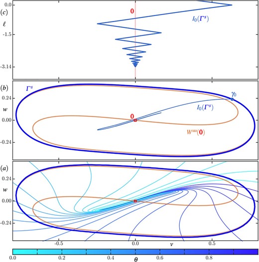
Details of isochron geometry in region F in the (rotated) |$(v, w)$|-plane. Panel ((a)) shows the phase portrait, consisting of  ,
,  , and
, and  , together with ten isochrons of
  , and panel ((b)) shows the phase portrait with only the zero-phase isochron
  ; here, each isochron in panel (|$a$|) is coloured according to its phase |$\theta $| as given by the colour bar. Panel (|$c$|) shows how the |$v$|-coordinate along
  changes with arclength |$\ell $| (asymptotically approaching |$\ell \approx -3.138$|), where the |$v$|-range is as in panels (|$a$|)and(|$b$|) and the red vertical line indicates the position
  with respect to the |$v$|-direction. Compare with Figs. 2 and 3.
3.7 Transition of the tangency orbits |$O_{\pm }$|
As was discussed in the previous sections, quadratic tangencies between forward-time and backward-time isochron foliations occur in regions B–D along the symmetric pair of tangency orbits |$O_{\pm }$|, and they are associated with sharp turns of one isochron foliation with respect to the other. Figure 16 presents series of sketches that illustrate how the tangency orbits |$O_{\pm }$| emerge, bifurcate and then disappear again in the transitions from regions |$\boldsymbol {B}--\boldsymbol {E}$|. Each panel shows (in rotated coordinates) the invariant objects of the representative phase portraits together with |$O_{\pm }$|, each labelled to indicate their respective bifurcation or region. Note that, in Figure 16, we are not showing the isochron foliations that become tangent along |$O_{\pm }$|; they can be found in Figure 3 and are described in Section 3.3 to Section 3.5.
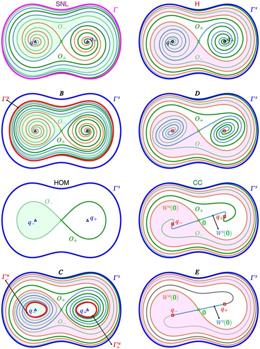
Sketches of the phase portraits of (1.10) that illustrate the changes of the isochron foliation tangency orbits  due to the bifurcation sequence studied. Phase portraits are sketched in the rotated |$(v, w)$|-coordinates and show all relevant invariant objects; see Figure 2 for details of the labelling.
The orbits |$O_{\pm }$| are created in the bifurcation |$\textbf {\texttt {SNL}}$| where a nonhyperbolic saddle-node periodic orbit |$\varGamma $| emerges. As |$\textbf {\texttt {SNL}}$| is approached from within region |$\boldsymbol {A}$|, the two branches of |$W^s(\boldsymbol {0})$| develop an increasing number of rotations near where |$\varGamma $| is about to emerge before going off to infinity. At the bifurcation |$\textbf {\texttt {SNL}}$| the stable manifold |$W^s(\boldsymbol {0})$|, and with it the basins of attraction |$\mathcal {A}\left (q_{\pm }\right )$|, are now confined to lie inside |$\varGamma $|, rather than extending to infinity. As a result, there are two orbits |$O_{\pm }$| along which one finds tangencies between the forward-time isochrons of |$q_{\pm }$| and the backward-time isochrons of |$\varGamma $| (which exist inside |$\varGamma $| as the limits of the isochrons of the hyperbolic periodic orbit |$\varGamma ^u$| in region |$\boldsymbol {B}$|). The two tangency orbits |$O_{\pm }$| are each other’s symmetric counterparts and spiral into |$q_{\pm }$| in forward time and accumulate on |$\varGamma $| in backward time, respectively. In region |$\boldsymbol {B}$| the nonhyperbolic periodic orbit |$\varGamma $| has split into |$\varGamma ^u$| inside |$\varGamma ^{s}$|, and |$O_{\pm }$| now accumulate on |$\varGamma ^u$| in backward time; inside the repelling periodic orbit |$\varGamma ^u$|, the situation is geometrically as at the bifurcation |$\textbf {\texttt {SNL}}$|, with a quadratic tangency between |$\mathcal {I}\left (q_{\pm }\right )$| and |$U_{0}(\varGamma ^u)$| along |$O_{\pm }$|.
As the homoclinic bifurcation |$\textbf {\texttt {HOM}}$| is approached, the stable and unstable manifolds |$W^s(\boldsymbol {0})$| and |$W^u(\boldsymbol {0})$| as well as the repelling periodic orbit |$\varGamma ^u$| and the tangency orbits |$O_{\pm }$| approach each other and pass very close to |$\boldsymbol {0}$|. At |$\textbf {\texttt {HOM}}$|, all these objects merge and form a lemniscate inside |$\varGamma ^u$|, as is sketched in Figure 16. In region |$\boldsymbol {C}$| the curves |$W^s(\boldsymbol {0})$| and |$W^u(\boldsymbol {0})$| have exchanged their relative positions, leading to the creation of the repelling periodic orbits |$\varGamma ^u_{\pm }$| on which |$W^s(\boldsymbol {0})$| and the tangency orbits |$O_{\pm }$| now accumulate in backward time; at the same time |$W^u(\boldsymbol {0})$| and |$O_{\pm }$| accumulate on |$\varGamma ^{s}$| in forward time. The quite spectacular effect of the transition at |$\textbf {\texttt {HOM}}$| is that the tangency along |$O_{\pm }$| is now between |$\mathcal {I}\left (\varGamma ^{s}\right )$| and |$\mathcal {U}(\varGamma ^u_{\pm })$|, while |$\mathcal {I}\left (q_{\pm }\right )$| and |$\mathcal {U}(\varGamma ^u_{\pm })$| intersect transversely inside |$\varGamma ^u$|.
At |$\textbf {\texttt {HB}}$| the equilibria |$q_{\pm }$| become hyperbolic repellors as the periodic orbits |$\varGamma ^u_{\pm }$| disappear. As a result, the two branches of the stable manifold |$W^s(\boldsymbol {0})$| and the tangency orbits |$O_{\pm }$| now converge to |$q_{\pm }$|. Since the equilibria |$q_{\pm }$| are foci, along |$O_{\pm }$| one finds in region |$\boldsymbol {D}$| (as well as at |$\textbf {\texttt {HB}}$|) the quadratic tangencies of the foliation |$\mathcal {I}\left (\varGamma ^{s}\right )$| and |$\mathcal {U}(q_{\pm })$|. Finally, at the transition |$(\textbf {\texttt {CC}})$| the eigenvalues of |$q_{\pm }$| become real and these equilibria lose their spiralling nature. Hence, the foliation |$\mathcal {U}(q_{\pm })$|, and with it the tangency orbits |$O_{\pm }$|, have disappeared in region |$\boldsymbol {E}$|. Our numerical investigations suggest that the limits of |$O_{\pm }$| are two orbits tangent to the emerging eigendirection of the weaker real eigenvalue in region |$\boldsymbol {E}$|, and approaching |$q_{\pm }$| from the direction opposite of |$W^s(\boldsymbol {0})$|; two such orbits are shown as grey curves in Figure 16.
4. Conclusions and outlook
We presented a case study of foliations of basins of attraction and repulsion by forward-time and backward-time isochrons, respectively, in a planar vector field. The emphasis was on the interactions of two such foliations in regions where both forward-time and backward-time isochrons exist, and how such interactions change during a quite typical sequence of bifurcations. We found that the respective isochron foliations associated with a pair of basins that wind onto a periodic orbit are forced to have quadratic tangencies along a unique tangency orbit in each of the winding basins. For the vector field we considered, the two winding basins are related by a rotational symmetry, but this is not actually a requirement from the topological point of view. The main point is that the isochrons of the attractor/repellor in any winding basin necessarily need to have tangencies with the other isochrons of the periodic orbit onto which it accumulates. As a result, one finds sharper and sharper turns in the tiny ‘channel’ of the winding basin. We showed how winding basins arise in a saddle-node or fold of periodic orbits and then bifurcate in a homoclinic bifurcation. The latter transition is quite spectacular, in that winding basins of attraction effectively change into winding basins of repulsion, with an associated change of the properties of the isochron foliations involved. The isochron foliation of the winding basin is lost after a Hopf bifurcation when the bifurcating equilibrium ceases to spiral.
These actual bifurcations of the vector field provide a second mechanism for generating nontransverse isochron foliations with structurally stable quadratic tangencies, namely, along a single tangency orbit in each basin. This is markedly different from the first mechanism reported by Langfield et al. (2015) of a cubic isochron foliation tangency or CIFT, where quadratic tangencies are generated along a pair of tangency orbits; in particular, a CIFT is not associated with a bifurcation. Identifying the different ways in which quadratic isochron tangencies and tangency orbits may arise when parameters are changed is not only interesting from a theoretical perspective, but also of practical importance: they are one way of explaining and identifying very sharp turns of (forward-time) isochrons (also referred to as boomerang turns (Osinga & Moehlis, 2010), or Z-shaped turns (Mauroy et al., 2014)) that are known indicators of extreme phase sensitivity.
Sharp or boomerang turns of isochrons have been observed in a reduced Hodgkin–Huxley system by Osinga & Moehlis (2010, Figs 3, 7 and 9, as well as in Morris–Lecar models by Guillamon & Huguet (2009, Fig. 4), Huguet & Llave (2013, Figs 3–4) and Pérez-Cervera et al. (2019, Fig. 13), and appear to be indicative of isochron foliation tangencies induced by a CIFT as shown by Langfield et al. (2015, Figs 5, 7, 8 and 10). In contrast, winding basins and the associated nontransversality of isochron foliations along a single tangency orbit emerge as generators of a different type of phase sensitivity. For example, Shaw et al. (2012, Fig. 9) present sharp turns (also for a constructed model) that appear to be induced by the basin boundary. Furthermore, the sharp turns present in the cross-sections of two-dimensional isochrons of the Hindmarsh–Rose model shown by Mauroy et al. (2014) appear to be organized geometrically as described here. Specifically, Figs 2(a), 2(b), 9 and 11 of (Mauroy et al., 2014) show isochrons with geometry similar to that seen in the basins |$\mathcal {U}(\varGamma ^{u}_{+})$| in Fig. 9(c), |$\mathcal {I}\left (q_{+}\right )$| in Figs. 4 and 6, |$\mathcal {I}\left (\varGamma ^{s}\right )$| in Figure 13 and |$\mathcal {I}\left (q_{+}\right )$| in Fig. 6(d), respectively.
Winfree’s initial motivation for studying isochrons was to get insight into the topology of phase resetting by |$\partial $|-function stimuli (Glass & Winfree, 1984; Winfree, 1967, 1974). He postulated that the map that transforms the old phase to a new phase, obtained when a fixed-amplitude stimulus is delivered at all phases of the cycle, must be continuous provided none of these stimuli lead to a point outside the basin of attraction of the limit cycle. A typical example of how a discontinuity arises would be a stimulus amplitude that maps a particular phase point along the limit cycle exactly onto the source singularity inside; the resulting phase map is then discontinuous and the associated graph is no longer comprised of a single, continuous, so-called resetting curve (Winfree, 1974). The examples considered here also have saddle equilibria with stable manifolds that do not lie in the basin of attraction. Any resetting stimulus that shifts a particular (old) phase to a point on or near the stable manifold of such a saddle equilibrium would have strong effects on the resulting resetting curves (Glass & Winfree, 1984). Thus, knowing the topology of isochrons and invariant sets leads directly to experimental predictions about the resetting curves. Recently developed methods (Langfield et al., 2020) now enable us to compute resetting curves as a continuous family parametrized by either the amplitude or phase at which the stimulus is applied. This means that one can now study the underlying mechanisms that deform the resetting curves from continuous curves with winding number 1 to discontinuous curves or curves with winding number 0; see (Langfield et al., 2020) for a more detailed discussion. These topological aspects can be studied experimentally, which offers an exciting direction of research that might help stimulate further experimental studies.
A take-home message of our work is that the generation of nontransverse isochron foliations via (global) bifurcations is a generic mechanism that must be expected to occur more generally. This clearly includes other planar vector field models, such as the Duffing oscillator and normal forms for resonance phenomena (Guckenheimer & Holmes, 1983; Kuznetsov, 2004). In short, winding basins and the associated nontransversality of isochron foliations along a single tangency orbit emerge as generators of a new type of phase sensitivity that does not require a time-scale separation between the variables. We deduce from the brief discussion of results by Shaw et al. (2012) and Mauroy et al. (2014) that our findings regarding interacting isochron foliations also have implications for the possible geometry of isochrons of higher dimensions. In particular, we expect that global bifurcations of codimension one, of which there are many more types already in dimension three, generate nontransversality between isochron foliations and associated phase sensitivity. However, new and more complex types of nontransversal isochron foliations should be expected; indeed, in three-dimensional vector fields one may expect topological changes of the two-dimensional isochrons that are as complex as those for two-dimensional invariant manifolds involved in organizing (chaotic) attractors. The study and classification of the topological and geometric properties of interacting foliations of two-dimensional isochrons remains an interesting and challenging topic for future research.
Finally, we mention that the investigation of the geometric properties of quite complicated isochron foliations, as presented here, has been made possible by a two-point BVP set-up (Langfield et al., 2014, 2015, 2020; Osinga & Moehlis, 2010) that has been refined and implemented in the package CoCo (Dankowicz & Schilder, 2009, 2013) as part of this project. The Matlab CoCo code is provided with a tutorial of two example computations as supplementary material with this paper—allowing the interested reader to adapt the code to compute isochrons in different (planar) examples. Ongoing work that will be reported elsewhere concerns finding the foliations by isochrons of two-dimensional stable and unstable manifolds of saddle periodic orbits in three-dimensional vector fields. The generalization of the BVP approach to the computation of two-dimensional isochrons in a three-dimensional phase space is possible in principle, but technically demanding since it requires generating and growing a two-dimensional mesh on a global manifold that is defined via a two-parameter family of orbit segments.
Acknowledgements
We thank Harry Dankowicz for helpful discussions and trouble-shooting while we were implementing the computation of planar isochrons within CoCo and Pablo Aguirre, Andrus Giraldo and Gemma Mason for advice regarding the computation of the curve |$(\textbf {\texttt {CC}})$|.
Funding
Royal Society Te Apārangi Marsden Fund (16-UOA-286 to B.K. and H.M.O.).
Footnotes
Winfree commonly refers to this concept as latent phase.
Made applicable to a periodic orbit by Irwin’s definition of stable (sub)manifolds of an elementary limit cycle (Irwin, 1970); see also (Hirsch et al., 1977).
First observed by Osinga and Moehlis (2010), these refer to the phenomenon when an isochron exhibits a relatively sharp turn and seemingly traces back along itself for a considerable arclength.
Specifically, the parameter |$\mu $| in (Hannam et al., 2016) is now set to 1; note that the value for |$b$| in (Hannam et al., 2016) was mistakenly given as |$b = 0.05> 0$|, it should have been |$b = -0.05 < 0$|.
The equilibria |$p_{\pm }$| are otherwise irrelevant to this case study; they emerge with a pair of sinks in a further saddle-node bifurcation, outside the range of Fig. 1.
The curve |$(\textbf {\texttt {CC}})$| can be computed by adapting the BVP suggested by Giraldo et al. (2017, Appendix B.2) to the case of equilibria.
Hence, the periodic orbits |$\varGamma ^{s}_{-}$| and |$\varGamma ^{u}_{+}$| are not invariant themselves, as |$\varGamma ^u$| was, but map to one another under the phase-space symmetry of (1.10) of rotation by |$\pi $| about the origin.
References
A. Dynamics at infinity
The phase portraits near infinity can be studied by compactifying phase space. This is achieved via Poincaré compactification (González-Velasco, 1969; Messias, 2009), which maps |$\mathbb {R}^{2}$| diffeomorphically to the open unit disc |$\mathbb {D}^{2}$| such that its boundary |$\mathbb {S}^{1}$| represents the direction of approach or departure from infinity; see also (Hannam et al., 2016) for more details and explicit formulas. This coordinate change preserves the geometry of invariant objects and results in a continuous vector field defined on a (bounded) closed unit disc |$\mathbb {D}^{2} \cup \mathbb {S}^{1}$|. Phase portraits in the compactification are equivalent to those in the original system, but with a nonlinear rescaling of time; here, points of |$\mathbb {S}^{1}$| correspond to direction of escape to infinity of the original system, which are determined by the higher-order terms.
Figure A17 shows compactified phase portraits in regions |$\boldsymbol {A}$|, |$\boldsymbol {B}$| and |$\boldsymbol {F}$|. The invariant objects on the unit circle |$\mathbb {S}^{1}$| representing infinity are unaffected by the linear terms of (1.10). Since the bifurcation parameter |$a$| only appears in the linear terms of (1.10), the dynamics on |$\mathbb {S}^{1}$| remain unchanged throughout regions |$\boldsymbol {A}--\boldsymbol {F}$|. On |$\mathbb {S}^{1}$| there are two nodal repellors |$q^{\infty }_{\pm } (0, \pm 1)$| and two saddles |$p^{\infty }_{\pm }$| at |$(\pm 1, 0)$|; their stable invariant manifolds |$W^s(p^{\infty }_{\pm })$| accumulate onto aerobic scope and trace out |$\mathbb {S}^{1}$|. The presence of the equilibria |$q^{\infty }_{\pm }$| and |$p^{\infty }_{\pm }$| on |$\mathbb {S}^{1}$| mean that trajectories of (1.10) do not spiral towards infinity, but escape to infinity (in forward or backward time) along the directions represented by the points aerobic scope and |$p^{\infty }_{\pm }$|. Hence, the only isochron foliations that we need to concern ourselves with are those of finite invariant objects.
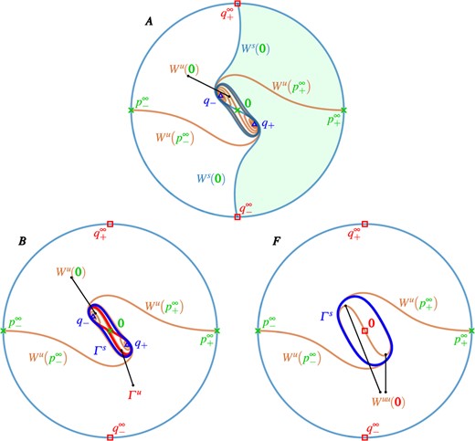
Compactified phase portraits of (1.10) in regions |$\boldsymbol {A}$|, |$\boldsymbol {B}$| and |$\boldsymbol {F}$|. The unit circle |$\mathbb {S}^{1}$| represents the direction of escape to infinity and consists two repellors  (
( ), two saddles
  (
( ) and their stable manifolds
  (blue curves). Also shown are the unstable manifolds
  (orange curves) and the respective finite invariant sets
  (
( ) and
) and  (
( ), with manifolds
  (light-blue curve),
  (orange curve) and
  (orange curve), and the periodic orbit
  (blue curve); compare with Figure 2.
The compactified phase portrait of region A in Fig. A17 shows that the two branches of |$W^s(\boldsymbol {0})$| accumulate in backward time to the repelling equilibria |$q^{\infty }_{-}$| and |$q^{\infty }_{+}$|, respectively. This shows that the curve |$W^s(\boldsymbol {0})$|, which forms the finite part of |$\partial \mathcal {A}\left (q_{\pm }\right )$|, winds around the equilibria |$\boldsymbol {0}$| and |$q_{\pm }$| only finitely many times. As a result, the (shaded) basin |$\mathcal {A}\left (q_{-}\right )$| encompasses most of the right-hand side of the image; in particular, the semicircle |$W^s(p^{\infty }_{+})$| is also in the boundary |$\partial \mathcal {A}\left (q_{-}\right )$|, and the equivalent statement is true for |$\mathcal {A}\left (q_{+}\right )$|. Hence, the isochron foliations |$\mathcal {I}\left (q_{\pm }\right )$| must accumulate onto both finite and non-finite invariant objects. Notice further that each basin |$\mathcal {A}\left (q_{\pm }\right )$| contains the unstable manifold |$W^u(p^{\infty }_{\mp })$| which, hence, converges in forward time to |$q_{\pm }$|.
In the compactified phase portrait of region B in Fig. A17 the pair of periodic orbits |$\varGamma ^{s}$| and |$\varGamma ^u$| now surround |$\boldsymbol {0}$| and |$q_{\pm }$|. Hence, |$W^s(\boldsymbol {0})$| accumulates onto |$\varGamma ^u$| in backward time and is no longer able to reach the points |$q^{\infty }_{\pm }$|, so that we now have a pair of winding basins of attraction |$\mathcal {A}\left (q_{\pm }\right )$| inside of |$\varGamma ^u$|. Similarly, the unstable manifolds |$W^u(p^{\infty }_{\pm })$| accumulate onto |$\varGamma ^{s}$| and no longer reach the attractors |$q_{\mp }$|. Note that the basin |$\mathcal {A}\left ({\varGamma ^{s}}\right )$| outside |$\varGamma ^{s}$| is bounded by the circle |$\mathbb {S}^{1}$|, that is, by the closure |$\overline {W^s(p^{\infty }_{-})} \cup W^s(p^{\infty }_{-})$|. The situation outside the stable periodic orbit |$\varGamma ^{s}$| remains unchanged in the transitions through regions |$\boldsymbol {C}$| to |$\boldsymbol {F}$|, as is illustrated in Figure A17 with the compactified phase portrait of region |$\boldsymbol {F}$|. Hence, any qualitative changes of isochron geometry from region |$\boldsymbol {B}$| onwards occur strictly inside |$\varGamma ^{s}$|.
B. Table of isochron properties across the transition
We summarize the transitions from regions A to F in a compact way in Table B3 (continued over three pages) in terms of the properties of the invariant objects and the isochron foliations in the different basins. This information is very dense and will be very hard to digest on a stand-alone basis; rather this summary is provided as a look-up table that the reader may wish to consult in conjunction with the detailed explanations in Section 3. Table B3 is organized into subtables for each region, separated by subtables for each of the transitions between them. Each subtable for a region presents all equilibria and periodic orbits, the invariant manifolds of saddle equilibria, the basins of attractors/repellors and their boundaries, and the properties of the relevant isochron foliations; we then list the intersections of basins of attraction and repulsion in which isochron foliations coexist, and denote whether the forward-time and backward-time isochron foliations are transverse or have quadratic tangencies. Each subtable for a transition indicates the bifurcation in terms of the invariant objects that characterize it, and then details the associated changes to invariant objects, basins and isochron foliations.
Summary of the phase portraits for regions A–F and the transitions between them. The subtables for each region present the respective label (first column), the invariant objects (second column) and their invariant manifolds for saddles and basins of attraction/repulsion, their boundaries and any isochron foliations (third column); we also indicate whether basins are unbounded or winding and list separately the intersection sets with interacting isochron foliations, where |$FX_here$| denotes transverse and |$FX_here$| tangent foliations. The subtables for each transitions between regions show the transition and bifurcating objects (first column) and then list the respective changes to the relevant invariant objects and foliations.
 |
|
Summary of the phase portraits for regions A–F and the transitions between them. The subtables for each region present the respective label (first column), the invariant objects (second column) and their invariant manifolds for saddles and basins of attraction/repulsion, their boundaries and any isochron foliations (third column); we also indicate whether basins are unbounded or winding and list separately the intersection sets with interacting isochron foliations, where |$FX_here$| denotes transverse and |$FX_here$| tangent foliations. The subtables for each transitions between regions show the transition and bifurcating objects (first column) and then list the respective changes to the relevant invariant objects and foliations.
|
|
continued.
 |
|
continued.
|
|
continued.
 |
|
continued.
|
|
