Limit theorems and phase transitions in the tensor Curie-Weiss Potts model Open Access

Abstract

1. Introduction

The Potts model [35], originally named after Renfrey Potts [32], is a generalization of the Ising model [25], where the spin of any particular site can have more than two states, each such state being referred to as a colour. It finds broad application in elucidating diverse physical phenomena, including magnetism, phase transitions and social behaviour. This model is related to a number of other well-known models, such as the Heisenberg model, the XY model and the Ashkin–Teller model (the four-state Potts model), and has found extensive applications in a number of diverse fields including biomedical problems [7, 28], image processing and computer vision [12, 26], spatial statistics [36], social sciences [9] and finance [8, 34]. The classical Potts model represents pairwise (quadratic) interactions between the sites, which, most often, is not enough to capture the complex dependencies present in real world network data. For example, in a peer group, the behaviour of an individual does not depend only on pairwise interactions between his/her friends, but is a function of more complex higher order interactions. In a different context, it is known in chemistry that the atoms on a crystal surface do not interact just in pairs, but in triangles, quadruplets and higher order tuples. A natural extension of the classical Potts model that captures multibody interactions, is the tensor Potts model, and in this paper, we consider the problem of deriving the asymptotics of a natural estimate of the parameters of this model, given only one sample from the model. Obtaining precise asymptotics of the sufficient statistic and the parameter estimates in general tensor Potts models is notoriously difficult, unless one agrees to assume certain special structures on the underlying network. One such natural structural condition is to assume that all tuples of nodes of a fixed order (say, |$p$|⁠) interact with each other, with a uniform interaction strength. The resulting model is the tensor Potts model on the |$p$|-uniform complete hypergraph, also referred to as the |$p$|-tensor Curie–Weiss Potts model.

A close relative of the Potts model is the Ising model [25], where there is a huge literature on the problem of consistent parameter estimation. Chatterjee [13] showed how to estimate the parameters of a general spinglass model consistently, using the idea of pseudolikelihood estimation, which was introduced by Besag [3, 4] in the context of spatial statistics. A myriad of works followed in the next few years on the problem of partial and joint estimation of Ising model parameters, some notable ones amongst them being [5, 16–18, 23]. In a rather different context, one might be interested in estimating the entire structure (interaction matrix) of a general Ising model, assuming that she has access to multiple samples from such a model. This problem is known as structure learning, and has been addressed in details in a series of works [1, 11, 27, 33]. The problem of deriving exact asymptotics of the magnetization and parameter estimates in the Curie–Weiss Ising model was addressed in [15, 20], and in [14] for Markov random fields on lattices. However, the Ising models in all these works capture only pairwise interactions, which as we discussed above, is often not a practical assumption in many realistic settings involving peer-group effects and multi-particle interactions. A natural substitute for the classical |$2$|-spin Ising model in such situations, is the |$p$|-spin Ising model [2, 10]. Consistent estimation of the natural parameters in general |$p$|-spin Ising models was established in [30], and exact fluctuations of the magnetization and parameter estimates were established for the |$p$|-spin Curie–Weiss model in [29, 31]. However, to the best of our knowledge, nothing is known about the asymptotics of the empirical magnetization vector and the parameter estimates for the closely related |$p$|-spin Potts model, even for the fully connected case, although the corresponding asymptotics have been established in the |$2$|-spin case in [19, 21, 22]. This is precisely the goal of this paper. We will see that even in this simple case where we have a |$p$|-spin Curie–Weiss Potts model, many surprising phase transitions arise in the asymptotics of the magnetization vector and the parameter estimates. Some salient features of these surprising phenomena include the appearance of rates of convergence (of the estimates) like |$N^{-3/4}$| and |$N^{-5/6}$| at some special points in the parameter space, and the existence of a smooth curve in the interior of the parameter space, where the estimates have limiting mixture distributions.

1.1 Model description

For integers |$p\ge 2$| and |$q\ge 2$|⁠, the |$p$|-tensor Potts model is a discrete probability distribution on the set |$[q]^{N}$| (here and afterwards, for a positive integer |$m$|⁠, we will use |$[m]$| to denote the set |$\{1,2,\ldots ,m\}$|⁠) for some positive integers |$q$| and |$N$|⁠, given by:

for all |$\boldsymbol X \in [q]^{N}$|⁠, where |$\beta>0$|⁠, |$h \geq 0$| and |$\boldsymbol J:= ((J_{i_{1}, \ldots ,i_{p}}))_{i_{1},\ldots ,i_{p}\in [N]}$| is a symmetric tensor. The |$p$|-tensor Curie–Weiss Potts model is obtained by taking |$J_{i_{1},\ldots ,i_{p}}:= N^{1-p}$| for all |$(i_{1},\ldots ,i_{p}) \in [N]^{p}$|⁠, whence model (1.1) takes the form:

where |${\bar{X}_{\cdot r}}:= N^{-1} \sum _{i=1}^{N} X_{i,r}$| with |$X_{i,r}:= \mathbb{1}_{X_{i}=r}$|⁠. The variables |$p$| and |$q$| are called the interaction order and the number of states/colours of the Potts model. A sufficient statistic for the exponential family (1.2) is the empirical magnetization vector:

Note that |${\bar{\boldsymbol X}_{N}}$| is a probability vector, i.e. has non-negative entries adding to |$1$|⁠. In this paper, we give a complete description of the asymptotics of |${\bar{\boldsymbol X}_{N}}$| on the entire parameter space:

We then use these asymptotics to establish limit theorems for the maximum likelihood (ML) estimators of |$\beta $| and |$h$|⁠, which is crucial for constructing asymptotic confidence intervals for these parameters.

1.2 Maximum likelihood estimation

Hereafter, given |$\boldsymbol X \sim \mathbb{P}_{\beta , h, p}$|⁠, we denote by |$\hat{\beta }_{N}$| and |$\hat{h}_{N}$| the marginal ML estimators of |$\beta $| and |$h$|⁠, respectively. It follows from Lemma S.7.1, that for fixed |$h \in \mathbb{R}, \hat{\beta }_{N}$| is a solution of the equation (in |$\beta $|⁠),

and for fixed |$\beta \in \mathbb{R}$|⁠, |$\hat{h}_{N}$| is a solution of the equation (in |$h$|⁠),

The limiting distribution of the ML estimates of |$h$| and |$\beta $| therefore depend on the fluctuations of the average magnetization |${\bar{\boldsymbol X}_{N}}$| across the parameter space |$\varTheta $|⁠. The main features of these asymptotics are highlighted below:

• The parameter space |$\varTheta $| has a subset of regular points, where the magnetization vector and the ML estimates are asymptotically normal, their rates of convergence being |$N^{-1/2}$|⁠.

• The complement of the set of regular points contains the so called critical points, which forms a continuous curve in the interior of the parameter space, on which the magnetization vector and the ML estimates have limiting mixture distributions, the latter consisting of continuous and discrete components.

• The remaining portion of the parameter space consists of exactly one special point, where the magnetization and the ML estimates have rates of convergence different from the classical |$N^{-1/2}$| rate. In case |$(p,q)\ne (4,2)$|⁠, the magnetization converges at rate |$N^{-1/4}$| and the parameter estimates at rate |$N^{-3/4}$| to limiting non-Gaussian distributions. On the other hand, if |$(p,q)=(4,2)$|⁠, the convergence rate of the magnetization at the special point changes to |$N^{-1/6}$|⁠, whereas the estimates converge at rate |$N^{-5/6}$|⁠. The estimates are thus superefficient at the special points.

Note that the |$N^{-5/6}$| convergence rate for the ML estimates is a special phenomenon noticed in the |$4$|-spin, |$2$|-colour Curie–Weiss Potts model, that is never observed in the closely related tensor Curie–Weiss Ising models, or in the classical |$2$|-spin Curie–Weiss Potts models. In Figs 4 and 5, we illustrate the different phase transitions through phase diagrams.

The rest of the paper is organized as follows: In Section 2, we describe the asymptotics of the magnetization vector of the |$p$|-spin Curie–Weiss Potts model. These asymptotics depend on the location of the parameters on one of the several components of a partition induced by the so called free energy function, mainly characterized by whether this function has one or multiple global maximizers, and what is the order of the first non-zero derivative at these maximizers. We use the results in Section 2 to derive limiting distributions of the ML estimators in Section 3. In Section 4, we use the results in Section 3 to derive asymptotic confidence intervals for the model parameters. In that section, we also summarize the partition of the parameter space into the regular, critical and special points as sketched above, in details. A brief sketch of the proofs of the main results in this paper is given in Section 5. Finally, complete proofs of all the results in the main paper are given in the supplement.

2. Asymptotics of the magnetization vector

In this section, we state our main results regarding the asymptotics of the magnetization vector. For this, we need a few definitions and notations. For |$p,q\ge 2$| and |$(\beta ,h) \in \varTheta $|⁠, the negative free energy function |$H_{\beta ,h}: \mathscr{P}_{q} \to \mathbb{R}$| is defined as:

where |$\mathscr{P}_{q}$| denotes the set of all |$q$|-dimensional probability vectors. We start by showing that the magnetization vector concentrates around the set |$\mathscr{M}_{\beta ,h}$| of all global maximizers of the function |$H_{\beta ,h}$|⁠. Actually, this and all the subsequent results in this section are proved under slightly perturbed versions of the model parameters.

Theorem 2.1 is proved in Supplementary S.1. It enables us to derive a law of large numbers of the magnetization vector towards the set |$\mathscr{M}_{\beta ,h}$| of global maximizers of |$H_{\beta ,h}$|⁠. We now derive the fluctuations of the magentization vector around |$\mathscr{M}_{\beta ,h}$|⁠, which depends, amongst other things, on the location of the point |$(\beta ,h)$| in the parameter space.

It is proved in Lemma S.6.3 in Supplementary S.6, that the above three subsets indeed form a partition of the parameter space |$\varTheta $|⁠. From Proposition S.6.1, it follows that the global maximizers of |$H_{\beta ,h}$| can be reparametrized as permutations of the vector

for some |$s \in [0,1)$|⁠, and hence, the problem can be reduced to a 1D optimization of the function |$f_{\beta ,h}(s): =H_{\beta ,h}(\boldsymbol x_{s})$|⁠. Note that the map |$s\mapsto \boldsymbol x_{s}$| is one–one, since |$s = 1-q x_{s,2}$|⁠.

We write |$f_{\beta ,h}(s)$| as,

where |$k(x)= k_{\beta ,p}(x):= \beta x^{p}-x\log x$|⁠. Hence, for |$\boldsymbol t \in \mathscr{H}_{q}$|⁠,

It is worth noting that Type-I special points were also observed in [22] for the classical |$p=2$| case. However, as we will see, Type-II special points appear in the case |$p=4, q=2$| only, and not when |$p=2$|⁠, due to some intricate properties of the function |$f_{\beta ,h,p}$|⁠. Specifically, the fourth derivative of this function around its maximizer is always non-zero for |$p=2$|⁠, and |$0$| only for |$(p,q)=(4,2)$|⁠. A detailed proof of this phenomenon can be found in Lemma S.6.2 of the supplement.

We now state our results regarding the central limit theorem (CLT) of the magnetization under the |$p$|-tensor Potts model with perturbed parameters. We begin with the CLT at regular points.

The proof of Theorem 2.2 is given in Supplementary S.2.1. Next, we state the CLT result at the critical points. The limiting covariance matrix indeed matches for the |$p=2$| case with that obtained in [21] and [22]. The results obtained in [21] are only for |$h=0$|⁠, and their function |$G_\beta $| is in fact, a dual of our function |$H_{\beta ,0,2}$|⁠, in the sense that the minimizers of the former function are maximizers of the latter and vice-versa (see Lemma A.1 in [6]). Moreover, while [22] allows |$|\beta _{n}-\beta |=o(1)$| and |$|h_{n}-h|=o(1)$|⁠, we restrict our analysis to |$|\beta _{n}-\beta |=O(1/\sqrt{N})$| and |$|h_{n}-h|=O(1/\sqrt{N})$|⁠. This restriction enables us to derive explicit expressions for the mean of the limiting distribution.

Theorem 2.3 is proved in Supplementary S.2.2. Note that the limiting covariance matrices in Theorem 2.3 match exactly with those in [22] for the case |$p=2$|⁠, since they are simply permutations of the covariance matrix in Theorem 2.2.

Finally, we state the CLT result at the special points. We start with the CLT for type-I special points.

Theorem 2.4 is proved in Supplementary S.2.3. This limiting distribution once again matches with the one appearing in Theorem 3.7 in [22] for the case |$p=2$|⁠. To conclude, we prove the CLT for Type-II special points.

Theorem 2.5 is proved in Supplementary S.2.4. In Figs 1–3, we compare the empirical distributions of the magnetization with their corresponding asymptotic theoretical distributions as stated in the above theorems, in each of the three cases where the true parameter is regular, critical and special. The simulations were performed for the case |$p=4, q=3$| with |$N = 1000$|⁠, using MCMC.

Fig. 1.

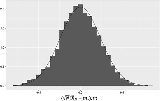
Histogram and theoretical density curve of |$\sqrt{N}({\bar{\boldsymbol X}_{N}}-\boldsymbol m_{*})$| projected at a random direction |$\boldsymbol v:= (0.157, 0.396, 0.323) $| at a regular point (⁠|$\beta =0.616$|⁠, |$h=0.67$|⁠).

Open in new tabDownload slide

Fig. 2.

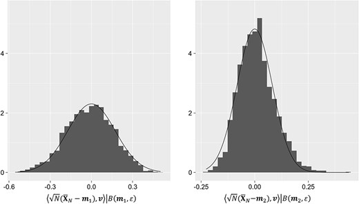
Conditional histograms and theoretical density curves of |$\sqrt{N}({\bar{\boldsymbol X}_{N}} - \boldsymbol m_{i})$| projected at a random direction |$\boldsymbol v:= (0.157, 0.396, 0.323)$| at a strongly critical point (⁠|$\beta =0.965$|⁠, |$h=0.2$|⁠).

Open in new tabDownload slide

Fig. 3.

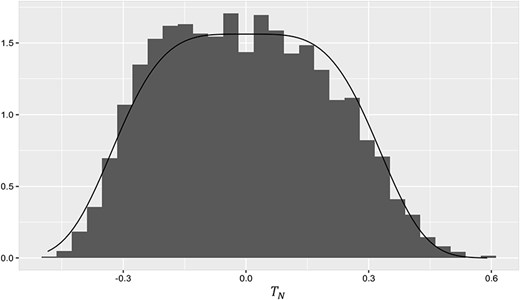
Histogram and theoretical density of |$T_{N}$| at the (Type-I) special point (⁠|$\beta =0.778$|⁠, |$h=0.485$|⁠).

Open in new tabDownload slide

3. Asymptotics of the maximum likelihood estimates

In this section, we prove results about the asymptotics of the ML estimates of the parameters |$\beta $| and |$h$|⁠. We define |$u_{N, p}$| and |$u_{N, 1}$| to be the functions appearing in the LHS of the equations (1.3) and (1.4), respectively, that is,

It follows from Lemma S.7.1 that for fixed |$h$|⁠, the ML estimate |$\hat{\beta }$| satisfies the equation:

and for fixed |$\beta $|⁠, the ML estimate |$\hat{h}$| satisfies the equation:

We start with the results about the asymptotic distribution of |$\hat{h}_{N}$|⁠, which depend on whether the underlying parameters are regular, special or critical.

Theorem 3.1 is proved in Supplementary S.3.1. It shows that |$\hat{h}_{N}$| is |$N^{\frac{1}{2}}$|-consistent and asymptotically normal at the regular points. Before discussing more about the implications of this theorem, we state the result for the asymptotic distribution of |$\hat{h}_{N}$| when |$(\beta , h)$| is special.

The proof of Theorem 3.2 is exactly similar to the proof of Theorem 3.1, so we skip it. It shows that at the Types-I and -II special points, |$\hat{h}_{N}$| is superefficient, and is |$N^{3/4}$| and |$N^{5/6}$|-consistent, respectively, and the limiting distributions are also non-Gaussian. We now state the result on the asymptotics of |$\hat{h}_{N}$| at the critical points. For this, we need a few definitions:

Theorem 3.3 is proved in Supplementary S.3.2. It shows that at the critical points, the limiting distribution of |$\hat{h}_{N}$| is a mixture distribution consisting of half-normal distributions and a point mass at |$0$|⁠. In particular, |$\hat{h}_{N}$| is always |$\sqrt{N}$|-consistent at the critical points. We now shift our attention to the asymptotics of |$\hat{\beta }_{N}$|⁠.

Theorem 3.4 is proved in Supplementary S.3.3. It shows that |$\hat{\beta }_{N}$| is |$N^{\frac{1}{2}}$|-consistent and asymptotically normal at the regular points when the maximizer is not |$\boldsymbol x_{0}$|⁠, whereas if the maximizer happens to be |$\boldsymbol x_{0}$|⁠, then |$N^{\frac{1}{2}}(\hat{\beta }_{N}-\beta )$| is inconsistent.

We omit the proof of Theorem 3.5 due to its close resemblance to the proof of Theorem 3.4. It is worth noting the difference between the two types of special points even in terms of the asymptotics of the ML estimates. While |$\hat{h}_{N}$| remains consistent at both these types of special points, |$\hat{\beta }_{N}$| becomes inconsistent at Type-II special points, whereas it still remains consistent at most type-I special points.

Finally, we state the result about the asymptotics of |$\hat{\beta }_{N}$| at the critical points.

Theorem 3.6 is proved in Supplementary S.3.4. It says that as long as |$(\beta ,h) \ne (\beta _{c},0)$|⁠, |$\hat{\beta }_{N}$| is |$\sqrt{N}$|-consistent, and its asymptotic distribution is either a mixture of half-normals and a point mass at |$0$|⁠, or just a normal, depending on whether the point is strongly or weakly critical, respectively. However, if |$(\beta ,0)=(\beta _{c},0)$|⁠, then |$\hat{\beta }_{N}$| is no longer |$\sqrt{N}$|-consistent, and a portion of the asymptotic mass escapes to |$-\infty $|⁠. The last phenomenon can be explained by the fact that for |$h=0$|⁠, if |$\beta <\beta _{c}$|⁠, |$\sqrt{N}(\hat{\beta }_{N}-\beta )$| does not have any asymptotic finite mass, and for |$\beta>\beta _{c}$|⁠, |$\hat{\beta }_{N}$| is |$\sqrt{N}$| consistent, so at the transition point |$\beta _{c}$|⁠, a portion of the asymptotic mass of |$\sqrt{N}(\hat{\beta }_{N}-\beta )$| is finite, and the remaining mass stays at |$-\infty $|⁠.

4. Confidence intervals for the model parameters

In this section, we start by summarizing the partition of the parameter space into different components, induced by the function |$H_{\beta ,h}$|⁠. This summary is a consequence of the results proved in Supplementary S.6. The existence of this partition and the different forms of the limiting distributions of the ML estimates on the different components of this partition gives rise to an inherent difficulty in constructing confidence intervals for the model parameters. In this context, there are two different scenarios:

• 1.

  |$\boldsymbol{p\ge 5 \ \ \mathbf{or}\ \, q\ne 2}$|⁠: In this case, the only special point in the parameter space |$({\widetilde{\beta }_{p,q}},{\widetilde{h}_{p,q}})$| lies in |$(0,\infty )\times (0,\infty )$|⁠. This point is Type-I special. The set |$\mathscr{C}_{p,q}^{1}$| is a smooth, strictly decreasing curve starting from the point |$({\widetilde{\beta }_{p,q}},{\widetilde{h}_{p,q}})$| (excluding it), and continuing till a point |$(\beta _{c}(p,q),0)$| (including it). The set |$\mathscr{C}_{p,q}^{2}$| is the interval |$\{(\beta ,0): \beta> \beta _{c}(p,q)\}$|⁠. The remaining portion of the parameter space |$\varTheta $| is the set of all regular points.

• 2.

  |$\boldsymbol{p\in \{2,3,4\},~ q= 2}$|⁠: In this case, any point |$(\beta ,h)$| with either |$h>0$| or |$\beta <\beta _{c}(p,q) = \frac{2^{p-1}}{p(p-1)}$| is a regular point. The point |$(\beta _{c}(p,q),0)$| is the unique special point, which is of Type-I if |$p\in \{2,3\}$|⁠, and Type-II if |$p=4$|⁠. The remaining portion of |$\varTheta $|⁠, i.e. the interval |$\{(\beta ,0): \beta> \beta _{c}(p,q)\}$| is the set |$\mathscr{C}_{p,q}^{2}$|⁠. Consequently, |$\mathscr{C}_{p,q}^{1} =\varnothing $| in this case.

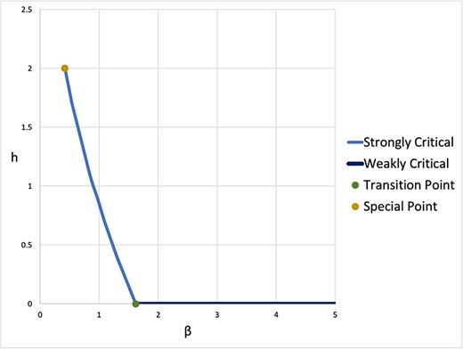
In Fig. 4, we illustrate this partition for the case |$p=7, q=5$|⁠, and in Fig. 5, for the case |$p=4,q=2$|⁠, through phase diagrams. One should note the following stark differences between the classically well-understood case |$p=2$| and the higher |$p$| case. First of all, for |$p=2$|⁠, type-II special points do not appear, unlike the case |$(p,q)=(4,2)$|⁠, and hence, sixth-order Gaussian asymptotics of the magnetization vector never arise in the former classical case. Secondly, in the |$2$|-colour model |$(q=2)$|⁠, higher-order Gaussian asymptotics of the magnetization can only occur in presence of a non-zero external field for |$p\ge 5$|⁠, whereas such asymptotics occur in the absence of any external field for |$p=2$| (and also for |$p=3,4$|⁠). Finally, the critical curve for the case |$p=2$| is a straight line (see Equation (2.4) in [22]) whereas for higher |$p$|⁠, linearity is not guaranteed.

Fig. 4.

Phase diagram for the case |$(p,q)=(7,5)$|⁠. The strictly decreasing part of the curve in the |$h>0$| region denotes the set of strongly critical points, the flat part of the curve (where |$h=0$|⁠) denotes the set of weakly critical points, the topmost extreme point of the curve denotes the special point (which in this case is of Type-I), and the point in the |$h=0$| axis at the junction of the strictly decreasing and flat parts of the curve denotes the transition point |$\beta _{c}$|⁠. The rest of the plain, which is the complement of all these curves, lines and points, is the set of regular points.

Open in new tabDownload slide

Fig. 5.

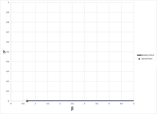
Phase diagram for the case |$(p,q)=(4,2)$|⁠. The flat line (with |$h=0$|⁠) denotes the set of weakly critical points, and the point at the left extremity of this flat line denotes the special point, which is of type II. The remaining region, which is the complement of these two sets, is the set of regular points.

Open in new tabDownload slide

We now discuss how to construct confidence intervals for the model parameters |$\beta $| and |$h$|⁠, with asymptotic coverage probability |$1-\alpha $|⁠. This is not a direct task, since the asymptotics of the ML estimates depend upon the exact position of the true |$(\beta ,h)$| in |$\varTheta $|⁠. However, intuitively speaking, since the complement of the set of regular points has Lebesgue measure |$0$|⁠, it should be enough to just use the limiting distributions at the regular points to construct the confidence intervals for the model parameters. So, let us imagine that an oracle told us beforehand that the unknown parameter |$(\beta ,h)$| is regular. Then, the intervals:

are asymptotic |$(1-\alpha )$|-coverage confidence intervals for |$h$| given |$\beta $|⁠, and |$\beta $| given |$h\ne 0$|⁠, respectively.

We now discuss how to modify the intervals |$I$| and |$J$| to asymptotically valid confidence sets at all points. Towards this, for every |$\beta $|⁠, let |$S(\beta )$| be the set of all |$h$|⁠, such that |$(\beta ,h)$| belongs to the closure of the set |$\mathscr{C}_{p,q}$|⁠, and for every |$h\ne 0$|⁠, let |$T(h)$| be the set of all |$\beta $|⁠, such that |$(\beta ,h)$| belongs to the closure of the set |$\mathscr{C}_{p,q}$|⁠. Note that both |$S(\beta )$| and |$T(h)$| have cardinality at most |$1$|⁠. Clearly, |$I\bigcup S(\beta )$| and |$J\bigcup T(h)$| are asymptotically level |$1-\alpha $| confidence sets for |$h$| given |$\beta $| and |$\beta $| given |$h\ne 0$|⁠, respectively, which have the same Lebesgue measure as the intervals |$I$| and |$J$|⁠, respectively.

There is an alternative, more precise two-step algorithm one can follow, than just uniting the points on the closure of the critical curve to |$I$| and |$J$| as described above, to get the universally valid confidence intervals. For fixed |$\beta $|⁠, one can first consistently test the null hypothesis |$H_{0}: h \in S(\beta )$| at level |$\alpha $| using the asymptotic distribution of |$\hat{h}_{N}$| at the critical or special points. If this null is rejected, then he can report |$I$| as the confidence interval for |$h$|⁠, and otherwise, he can declare the singleton set |$S(\beta )$| as the confidence interval (which is either empty, or just a point). A similar approach can be followed for constructing the confidence interval for |$\beta $| also, where this time, one tests the null hypothesis |$H_{0}: \beta \in T(h)$| in the first step, and if this is accepted, reports |$T(h)$| as the confidence interval for |$\beta $|⁠, and |$J$| otherwise.

5. Sketch of proof

In this section, we provide a brief sketch of the proofs of the main results in this paper. We begin with the proof of the asymptotics of the magnetization vector. Our derivation of the limiting distributions for the magnetization vector builds upon ideas from [22]. However, while [22] leverages specific properties of the maximizers of the free energy function |$f_{\beta ,h}$| for |$p=2$| (see their Theorem 2.3), such properties were not readily available in the literature for |$p>2$|⁠. A careful analysis was therefore necessary to establish these properties for the general case. On the other hand, the model in [21], in addition to being restricted to the |$p=2$| case, did not incorporate any external field term either, and hence, the interesting 2D phase transition phenomena were not revealed in their paper. Also, note that unlike [22] and our paper, in the setting of [21] (⁠|$p=2$|⁠, |$h=0$|⁠, |$q\ge 3$|⁠), no special points exist where higher-order Gaussian type of asymptotics for the magnetization vector arise.

The first step towards proving asymptotics of the magnetization vector, is to show that the magnetization vector concentrates around the set of all global maximizers of the function |$H_{\beta ,h}$|⁠, which makes them natural candidates for centering in the central limit theorems. The next step is to show that conditional on the event that |${\bar{\boldsymbol X}_{N}} $| is some neighbourhood of a global maximizer |$\boldsymbol m_{*}$| whose closure is devoid of any other maximizer, every bounded, continuous function |$g:\mathbb{R}^{q} \to \mathbb{R}$|⁠, satisfies:

where |$Y$| follows the law of the appropriate limiting distribution (which is either a Gaussian, or a fourth-order or sixth-order Gaussian, depending on whether the true parameter is regular/critical or special). A subsequent uniform integrability argument for all moments of |$\sqrt{N}({\bar{\boldsymbol X}_{N}} - \boldsymbol m_{*})$| will now imply its weak convergence and convergence in all moments to |$Y$|⁠. With the vision of applying these results to derive the asymptotics of the ML estimates, we prove these convergence results under slightly perturbed versions of the true parameters, the perturbations being of the order |$N^{-1/2}$|⁠.

The results on the asymptotics of the ML estimates in our paper are completely new, and have not appeared in, for example, [21, 22]. For proving these results, using monotonicity of the functions |$u_{N,1}$| and |$u_{N,p}$|⁠, one can express the cumulative distributions of |$\sqrt{N}(\hat{h}_{N} - h)$| and |$\sqrt{N}(\hat{\beta }_{N}-\beta )$| in terms of the cumulative distributions of |$\sqrt{N}(\bar{X}_{\cdot 1} - m_{*1})$| and |$\sqrt{N}(\|{\bar{\boldsymbol X}_{N}}\|_{p}^{p} - \|\boldsymbol m_{*}\|_{p}^{p})$| at their respective expectations under the perturbed parameters. This then enables one to translate the asymptotic results of |${\bar{\boldsymbol X}_{N}}$| to asymptotics of the ML estimates. Some care needs to be cautioned at critical points where there are more than one maximizer, but in that case, the leaning of |${\bar{\boldsymbol X}_{N}}$| towards some particular maximizers and away from the others, is largely governed by the sign of the perturbation of the true parameters, which is made rigorous through some perturbative concentration results proved in Supplementary S.5.

Acknowledgements

The authors wish to thank the editor, and the anonymous referee for their insightful comments, which greatly improved the quality and the presentation of the paper.

Funding

National University of Singapore start-up grant WBS A0008523-00-00 to S.M. and the FoS Tier 1 grant WBS A-8001449-00-00 to S.M.

Data availability

No real data were analyzed in this paper.

References