


Abstract
With high temperature becoming an increasing health risk due to a changing climate, it is important to quantify the scale of the problem. However, estimating the burden of disease (BoD) attributable to high temperature can be challenging due to differences in risk patterns across geographical regions and data accessibility issues.
We present a methodological framework that uses Köppen–Geiger climate zones to refine exposure levels and quantifies the difference between the burden observed due to high temperatures and what would have been observed if the population had been exposed to the theoretical minimum risk exposure distribution (TMRED). Our proposed method aligned with the Australian Burden of Disease Study and included two parts: (i) estimation of the population attributable fractions (PAF); and then (ii) estimation of the BoD attributable to high temperature. We use suicide and self-inflicted injuries in Australia as an example, with most frequent temperatures (MFTs) as the minimum risk exposure threshold (TMRED).
Our proposed framework to estimate the attributable BoD accounts for the importance of geographical variations of risk estimates between climate zones, and can be modified and adapted to other diseases and contexts that may be affected by high temperatures.
As the heat-related BoD may continue to increase in the future, this method is useful in estimating burdens across climate zones. This work may have important implications for preventive health measures, by enhancing the reproducibility and transparency of BoD research.
A general framework to calculate the burden of disease (BoD) attributable to high temperatures as measured by disability-adjusted life-years (DALYs).
Hands-on methodology for estimating the heat-attributable BoD considering climatic variations and population distribution.
A transparent method for estimated current burden of disease and future projections with clear assumptions.
Background
Quantifying the burden of disease (BoD) associated with specific risk factors is important, as this provides timely and policy-relevant information to inform needed actions toward improving health.1 The Global Burden of Disease (GBD) study, which has been conducted periodically since 1996, was among the first attempts to estimate the magnitude of health loss associated with a variety of diseases, injuries and population risk factors.2,3 Studies have estimated the BoD attributable to environmental health risk factors, including ambient and indoor air pollutants, unsafe water, lead and occupational exposures.4,5 The GBD study of 2019 assessed 87 risk factors, with major updates to environmental health risk factors by including non-optimal temperature exposure.3 Generally, these studies follow a similar methodological approach in applying risk functions to simulated exposure distributions across populations under specific scenarios.6–9
In response to the GBD study, several countries have developed independent BoD studies that aim to provide evidence tailored to their national circumstances.10–13 However, given the complexity in the BoD approach and differences in availability of data sources, purposes and methods, flexible strategies are required to facilitate interpretation and application of the most appropriate data in the national context.14,15 Recently, concerns have been raised about the limited interaction and collaboration between environmental epidemiologists and BoD researchers, and about the currently limited coverage of environmental health risk factors by the GBD project.16 In addition, specific challenges are involved in the estimation of BoD attributable to environmental health risk factors. For example, assumptions need to be made regarding uncertainties related to the patterns of health risks associated with particular environmental health risk factors and the variability in confounding factors and exposure distributions in the population.17 There are also inherent limitations in data sources which may constrain the accuracy of environmental BoD estimates.18
Global climate change is one of the most pressing environmental challenges that humans will face in the coming decades.19 Extreme heat, a significant environmental risk factor that has wide-ranging negative impacts on human health, is expected to become more frequent and intense worldwide.19 The excess morbidity and deaths associated with the effects of ambient heat exposures are well documented. Although studies have estimated the health impacts attributed to heat exposure using years of life lost (YLL),20 relatively few have used disability-adjusted life-years (DALYs) as their outcome indicator, perhaps because such studies are highly dependent on the availability of years lived with disability (YLD) data.16 By taking the severity of disease and age at death into account, and allowing inclusion and comparison of both non-fatal and fatal outcomes, DALYs are considered to be an important summary measure for population health and health policy planning.2,3,10 However, there is a lack of a structured illustration that lays out the key steps in quantifying the heat-related BoD.6,9 To address these concerns, we outline the steps involved and define the assumptions that need to be made when using high temperatures as an environmental health risk factor. Following the method used by the Australian Burden of Disease Study led by the Australian Institute of Health and Welfare,10 the present methodology comprises two steps (Figure 1). First, we estimate the population attributable fractions (PAF) using relative risks of the exposure-response relationship classified according to the Köppen–Geiger climate system,21 the exposure associated with the lowest conceivable risk to the population (theoretical minimum risk exposure distribution, TMRED), and exposure levels of the risk factor. Second, we calculate the BoD attributable to high temperatures, incorporating YLL and YLD to obtain climate-specific and national attributable DALYs. The methodology used will be demonstrated by using a case study: estimating the suicide and self-inflicted injuries burden attributable to high temperatures in Australia.
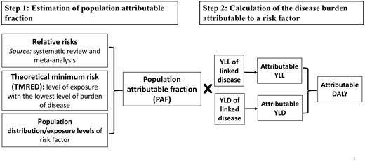
Inputs and steps in the calculation of the disease burden attributable to a risk factor. YLL, years of life lost; YLD, years lived with disability; DALY, disability-adjusted life-years. Adapted from Australian Burden of Disease Study 201810
Methods
Case study
Suicide is a complex psychopathological phenomenon influenced by biological, psychological, social (traumatic and stressful events) and environmental factors (seasonality, green spaces).22 As one source of environmental factors, high temperatures have been linked to suicide and self-inflicted injuries risks across different geographical and climatic regions.22 Although there is mixed evidence in regards to the shape of the association (linear and non-linear), consistent findings have suggested that higher temperatures are associated with an increase in the risk of suicide.22–24 A plausible explanation is that changes in biochemical reactions (e.g. serotonin function) during extreme heat contribute to the build-up of compound stress, which can lead to mental conditions such as aggression, impulsiveness and suicidal tendencies.22–24
Climate classification based on seasons and environmental variables can be useful in determining temperature-related health outcomes.21,25 The Köppen–Geiger climate system uses precipitation and temperature to delineate climate types across the globe and has been used extensively in environmental and ecology research, and recently in health-related studies.21,22,25–29 We therefore propose that a paradigm matching exposure-response relationships by climate zone is useful in determining the global burden of temperature-sensitive diseases.28
As Australia is an expanse of about 7.69 million square kilometres encompassing a range of climate features, it is unreasonable to assume homogeneity in temperature exposure. We therefore stratified our analyses by 12 Köppen–Geiger climate zones across the country,21 each consisting of between five and 854 spatial areas, referred to as Statistical Areas Level 2 (SA2) in Australia. According to the Australian Bureau of Statistics, each SA2 (approximately a suburb) represents a community that interacts together socially and economically, with populations between 3000 and 25 000, although less in remote areas.30
Data acquisition
The reference period is the first factor to consider, as it serves as the basis for subsequent assumptions.31Figure 1 illustrates the several data sources required for calculating the attributable BoD. Ideally, all the required data would be available for the reference period, be it a single year or multiple years. For exposure-response relationships, the best available epidemiological evidence of the relative risk of the disease at the exposure site is obtained. We describe in the next section our systematic literature review and meta-analysis of evidence of the association required for the analysis.
In this case study, we examined the impact of high temperatures using the reference year 2003. We obtained gridded daily maximum and minimum temperature data from the Scientific Information for Land Owners interpolated climate raster datasets, with 0.05° × 0.05° (about 5 km × 5 km) spatial resolution, and calculated daily mean temperature.32 We then spatially interpolated these raster meteorological data and processed them at SA2 level. Using geographical information system techniques, we aligned the SA2 map with the climate zone map for Australia, thereby assigning the temperature and population information at the SA2 level (n = 2310) to different climate zone regions (n = 12). Population data at SA2 level were obtained from the Australian Bureau of Statistics to calculate a weighted BoD.33
Data on the annual burden of linked diseases [i.e. fatal burden (YLL) and non-fatal burden (YLD)] are required in the calculation of attributable BoD (Figure 1). For this case study, data on suicide and self-inflicted injuries (International Classification of Diseases, ICD-10: X60-X84, Y87.0) in 2003, at both state and national levels, were sourced from the Australian Institute of Health and Welfare.10
Step 1: estimation of population attributable fraction (PAF)
The estimation of PAF requires three inputs: (i) effect size estimation, (ii) TMRED detection and (iii) exposure level of risk factors. A detailed description of each of these inputs is given below.
Estimation of effect size (relative risks)
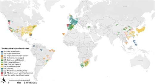
The first input involved in calculating the PAF is the effect size that expresses the strength of the association between the level of exposure to a risk factor and a disease outcome (relative risk per unit increase in exposure). Previous studies have shown that ambient temperature is associated with increased risk of population mortality and morbidity, often exhibiting a J-, V-, or U- shaped curve, with a positive association above and/or below a specific temperature or temperature range.24,34 In this study investigating the impacts of high temperature on suicide and self-inflicted injuries,22 we assume a constant log-linear increase in relative risk per unit increase in temperature above the defined TMRED.27,35,36 Due to the lack of some relevant Australian studies showing the association between high temperatures and suicide morbidity/mortality using finer temporal resolution data (i.e. daily data), we estimated the relative risk using data from recently published international systematic reviews22,24 and epidemiological studies.37–39 In these articles, each study location was assigned to a Köppen–Geiger climate zone21 as a proxy indicator for climate factors affecting health risk associated with high temperatures.25,28,40 The study locations varied widely, from Asia and Europe to North and South America, and included 328 estimates from international cities that lie within the 12 climate zones represented in Australia (Figure 2). We then calculated the pooled relative risk (per 1°C increase) for each climate zone using random-effect meta-analysis22,27,35 conducted using the ‘metan’ package in Stata (version 15.0). Table 1 summarizes the results.
Random-effect meta-analysis estimates of the relative risk (RR) and 95% confidence interval (CI) for risk of suicide per 1 °C increase in temperature for different Köppen–Geiger climate zones in Australia
| Climate zones | RR (95% CI) | k | I2, P-value | N |
|---|---|---|---|---|
| Af: Tropical rainforest | 1.020 (0.987-1.053) | 6 | 0.0%, P = 0.616 | 8360 |
| Am: Tropical monsoon | 1.162 (1.099-1.225) | 3 | 0.0%, P = 0.652 | 6511 |
| Aw: Tropical savanna (dry-winter) | 1.114 (1.005-1.223) | 11 | 33.9%, P = 0.127 | 12 010 |
| BSh: Hot semi-arid (steppe) | 1.022 (0.982-1.063) | 11 | 12.9%, P = 0.322 | 4862 |
| BSk: Cold semi-arid (steppe) | 1.022 (1.010-1.035) | 31 | 7.3%, P = 0.351 | 22 878 |
| BWh: Hot arid (desert) | 1.033 (1.008-1.058) | 4 | 0.0%, P = 0.893 | 5008 |
| BWk: Cold arid (desert) | 1.025 (0.971-1.078) | 3 | 0.0%, P = 0.638 | 1378 |
| Cfa: Humid subtropical | 1.027 (1.023-1.030) | 157 | 34.7%, P = 0.000 | 1 070 935 |
| Cfb: Oceanic | 1.052 (1.049-1.055) | 57 | 85.3%, P = 0.000 | 652 133 |
| Csa: Mediterranean hot summer | 1.038 (1.018-1.057) | 23 | 0.0%, P = 0.967 | 14 727 |
| Csb: Mediterranean warm/cool summer | 1.005 (0.981-1.030) | 14 | 0.0%, P = 0.503 | 5668 |
| Cwa: Dry-winter humid subtropical | 1.029 (1.009-1.048) | 8 | 46.2%, P = 0.072 | 27 892 |
As concerns could be raised about whether relative risks from studies conducted in climate zones in other countries would be relevant to Australian climate zones, we conducted a series of sensitivity analyses. We first identified the location-specific predictors (i.e. gross domestic product per capita, the annual average mean temperature, latitude and longitude) that might explain the heterogeneity for the included 328 estimates.9 We then conducted a meta-regression analysis as explained in the Supplementary Material (p. 1), available as Supplementary data at IJE online. The fitted meta-regression was then used to predict the adjusted relative risk for the Australian context. Analysis was conducted using the adjusted relative risk, and results can be found in Supplementary Table S1 (available as Supplementary data at IJE online). Second, we conducted sensitivity analyses using the non-linear functional forms (quadratic and cubic) of the exposure-response associations (see Supplementary Table S2, available as Supplementary data at IJE online). We also conducted a third sensitivity analysis using relative risks from local research—i.e. an Australian study, which used monthly (rather than daily) temperature data (see Supplementary Table S3, available as Supplementary data at IJE online).41
Theoretical minimum risk exposure distribution
The second input involved in calculating the PAF is the TMRED (also known as the theoretical minimum risk exposure level, TMREL). Following the comparative risk assessment framework,18 the estimated contribution of a risk factor to the BoD is calculated by comparing the observed exposure distribution with a counterfactual scenario (the TMRED). Specifically, the TMRED is the exposure at which the rate of the outcome is lowest, or the theoretical level of minimum risk in a population.10
The TMRED was the temperature at which the lowest risk of suicide and self-inflicted injuries occurs (minimum cause-specific mortality/morbidity temperature, MMT). Unlike other risk factors included in the GBD which have a fixed TMRED that applies to the whole population examined (e.g. occupational exposures and carcinogenic hazards),3,16 the TMRED for ambient temperature varies between locations due to diverse climate characteristics, temperature distributions, population characteristics (age, underlying medical conditions, socioeconomic status etc.) and other location-specific causes (rural or urban landscape, and infrastructure characteristics).42–43 Ideally, MMTs are determined by exposure-response curves, but this relies on the availability of data in a particular area.42 In the absence of such data allowing us to calculate MMT at each SA2 within specific climate zones in Australia, alternative approaches were explored to estimate the TMRED.28,42,44 In this case study, the most frequent daily mean temperature (MFT) was selected as a surrogate for MMT in each climate zone, based on the very close values and the unchanged MFT-MMT association reported in previous studies.42,45 This approach is supported by other studies showing that locations with higher mean temperatures tend to have higher optimal temperatures in association with disease outcomes.24,35 Other temperature metrics, such as annual mean temperature or annual median temperature, may be used as an alternative TMRED as appropriate.28,44 Sensitivity analyses were therefore conducted for a better understanding of the potential uncertainty of TMREDs (Supplementary Tables S4–S8, available as Supplementary data at IJE online).
Exposure levels of risk factor and associated effect size
The third input involved in the calculation of the PAF is the distribution of exposure, or exposure level prevalence (P) of the risk factor. For estimating the proportion of the year at each level of risk, it is crucial to have a clear and consistent definition of the unit of exposure.46
In our case study the risk factor was high temperature, and exposure to temperatures above the TMRED was assumed to be a risk factor for suicide. Therefore, the proportion of days with a mean daily temperature higher than the TMRED within a year was grouped in 1°C increments. The associated relative risks per unit (X degrees of temperature) were calculated, assuming a log-linear relationship between relative risk and temperature (Figure 3).35 We then multiplied the natural log relative risk by X before applying the exponential function.27,47 Thus the relative risk at temperature category c in zone z is given by Equation 1:
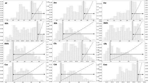
Histograms showing the distribution of mean ambient temperature in each climate zone across Australia in 2003. The arrows represent exposure levels of high temperature among population in 1-°C increments above the selected theoretical minimum risk exposure distribution (most frequent temperature, MFT). The dash-dot lines show how the relative risk increases above the MFT (solid line). Af, tropical rainforest; Am, tropical monsoon; Aw, tropical savanna (dry-winter); BSh, hot semi-arid (steppe); BSk, cold semi-arid (steppe); BWh, hot arid (desert); BWk, cold arid (desert), Cfa, humid subtropical; Cfb, Oceanic; Csa, Mediterranean hot summer; Csb, Mediterranean warm/cool summer; Cwa, dry-winter humid subtropical. Left axis, percentage; right axis, relative risk
Figure 3 presents the results of the high temperature exposures above the MFT, and the increase in relative risk of suicide and self-inflicted injuries in each climate zone. Supplementary Figure S1 (available as Supplementary data at IJE online) shows other TMREDs used for determining high temperature exposure levels.
Population attributable fraction (PAF) for heat-related health outcomes
The PAF determines the proportion of disease burden that could potentially have been prevented if exposure to a risk factor were reduced to an alternative ideal exposure scenario.8,35 The PAF is calculated by using the relative risk and the exposure level (P) of the risk factor (Equation 2 below).
As there were multiple exposure levels and associated relative risks in our case study, the products in the numerator and denominator were summed. For each climate zone we calculated the PAF using the following formula for a risk factor that has multiple categories of relative risks and exposure levels of mean temperature in 2003 (Equation 2): where ∑c is the sum over all categories, c is an index for exposure level category, P is the proportional exposure at each exposure level (i.e. the proportion of ‘hot’ days above the TMREDs in the reference year) and RRc is the relative risk specific to the temperature category as defined above.
Step 2: estimation of burden of disease attributable to high ambient temperature
The attributable BoD is the product of the PAF calculated in Step 1 and the national BoD data (YLL, YLD, DALY) weighted by population in the spatial area.33 We multiplied YLL and YLD with PAFs for each climate zone group, and the total attributable DALY is derived from the sum of the burden across all zones, using the following formula (Equation 3): where the YLL and YLD are sourced from the Australian Institute of Health and Welfare BoD databases. ∑i is the sum over all categories, i is an index for climate zone category, PAFYLLi is the mortality population attributable faction for category i, YLLi is the fatal burden of the category i, PAFYLDi is the morbidity population attributable fraction for category i and YLDi is the non-fatal burden of the category i.
In this case study, we calculated the proportion of the national population residing in each climate zone. We then multiplied this fraction by the BoD metric for suicide and self-inflicted injuries, obtained from the Australian Burden of Disease Study,46 to obtain the weighted DALYs. To estimate the heat-attributable BoD, DALY was multiplied by PAF for each climate zone to generate the total heat-attributable DALY. Table 2 shows the PAFs due to high temperature exposure, and the heat-attributable burden of suicide and self-inflicted injuries per climate zone across Australia. Results for sensitivity analyses using adjusted relative risk, different functional forms of exposure-response associations (linear and non-linear) and TMREDs for exposure levels are attached in Supplementary Tables S1–S8.
Summary statistics, population attributable fractions (PAFs) and heat-attributable burden of suicide by climate zone in Australia, 2003
| Climate zones | Population | MFT (°C) | Burden weighted by population | PAFs (%) | Heat-attributableburden | Heat attributable burden(per 10 000 population) | ||||||
|---|---|---|---|---|---|---|---|---|---|---|---|---|
| YLL | YLD | DALY | YLL | YLD | DALY | YLL | YLD | DALY | ||||
| Af: Tropical rainforest | 22 572 | 24.75 | 116.1 | 1.3 | 117.3 | 1.4 | 1.6 | 0.02 | 1.6 | 0.7 | 0.01 | 0.7 |
| Am: Tropical monsoon | 152 726 | 26.76 | 785.2 | 8.5 | 793.7 | 5.3 | 41.6 | 0.5 | 42.1 | 2.7 | 0.03 | 2.8 |
| Aw: Tropical savanna (dry-winter) | 443 317 | 27.33 | 2279.2 | 24.5 | 2303.8 | 6.2 | 141.3 | 1.5 | 142.8 | 3.2 | 0.03 | 3.2 |
| BSh: Hot semi-arid (steppe) | 293 252 | 27.64 | 1507.7 | 16.2 | 1523.9 | 0.6 | 9.05 | 0.1 | 9.1 | 0.3 | 0.00 | 0.3 |
| BSk: Cold semi-arid (steppe) | 1 711 924 | 12.17 | 8801.5 | 94.7 | 8896.2 | 10.0 | 880.2 | 9.5 | 889.6 | 5.1 | 0.06 | 5.2 |
| BWh: Hot arid (desert) | 222 814 | 26.78 | 1145.6 | 12.3 | 1157.9 | 2.2 | 25.2 | 0.3 | 25.5 | 1.1 | 0.01 | 1.1 |
| BWk: Cold arid (desert) | 99 324 | 11.1 | 510.7 | 5.5 | 516.1 | 14.0 | 71.5 | 0.8 | 72.3 | 7.2 | 0.08 | 7.3 |
| Cfa: Humid subtropical | 8 647 189 | 21.52 | 44 457.7 | 478.4 | 44 936.1 | 1.1 | 489.03 | 5.3 | 494.3 | 0.6 | 0.01 | 0.6 |
| Cfb: Oceanic | 5 390 304 | 9.6 | 27 713.1 | 298.2 | 28 011.3 | 23.2 | 6429.4 | 69.2 | 6498.6 | 11.9 | 0.13 | 12.1 |
| Csa: Mediterranean hot summer | 1 775 819 | 14.11 | 9130.0 | 98.2 | 9228.2 | 17.1 | 1561.2 | 16.8 | 1578.0 | 8.8 | 0.09 | 8.9 |
| Csb: Mediterranean warm/cool summer | 852 701 | 10.54 | 4384.0 | 47.2 | 4431.2 | 2.4 | 105.2 | 1.1 | 106.3 | 1.2 | 0.01 | 1.2 |
| Cwa: Dry-winter humid subtropical | 108 795 | 26.69 | 559.4 | 6.0 | 565.4 | 0.4 | 2.2 | 0.02 | 2.3 | 0.2 | 0.00 | 0.2 |
| National | 19 720 737 | – | 101 390 | 1091 | 10 2481 | – | 9757.6 | 105 | 9862.6 | 4.9 | 0.05 | 5.0 |
MFT, most frequent temperature; YLL, years of life lost; YLD, years of healthy life lost due to disability; DALY, disability adjusted life-years. PAFs, population attributable fractions.
Discussion
This methodology offers a general framework for calculating the PAFs and heat-attributable BoD which accounts for climatic variations and population distribution. Our method comprises two steps. First, the PAF for a health outcome associated with high temperatures, the environmental health risk factor, is estimated for the climate zones in the study region. Second, the heat-attributable burden is estimated by calculating the weighted DALYs according to population size and multiplying by the PAFs.
By using the best available epidemiological evidence from previous literature and local BoD data, we described the key steps to calculate heat-attributable BoD, through a practical example of an applied analysis. Our case study revealed the burden of suicide and self-inflicted injuries attributed to high temperatures within Australia. With MFT as the designated TMRED, the national heat-attributable suicide and self-inflicted injuries burden for 2003 was 5.0 DALYs per 10 000 population, with the highest rate of heat-attributable suicide in Oceanic (12.1 per 10 000 population) and Mediterranean hot summer (8.9 per 10 000 population) climate zones and the lowest in dry-winter humid subtropical climate zones (0.2 per 10 000 population) (Table 2). Despite heterogeneity across the climate zones, the heat-attributable burden of suicide was found to be higher in areas with higher temperature variability (Cfb-Oceanic, Csa-Mediterranean hot summer, BWk-Cold arid and BSk-Cold semi-arid climate zones) and relatively low MFTs. This suggests areas with a higher number of days of heat exposure generally showed more pronounced impacts.
Key assumptions and uncertainties in the methodology
The approach outlined here details the data and calculations required in estimating the heat-attributable BoD, but several assumptions need to be made, particularly if specific data on the exposure/health outcome association in the study population are not available. By explicitly stating these assumptions and uncertainties, which mainly concern the estimation of the relative risks and the determination of the TMRED, a transparent evaluation of the quality of the estimates can be made.
First, in the absence of local research to define the relative risks, the estimates can be sourced from systematic reviews of previous literature.10,48 A meta-analysis of relative risks reported in studies within certain climate zones can then be undertaken. Although the reviewed literature may include a limited number of estimates from a climate zone, we make the assumption that the pooled relative risk represents the relative risk occurring in association with a 1°C increase in temperature at any location within that climate zone. When there are no reported risk-outcome data available for a climate zone of interest, we make the assumption that the relative risks of a ‘similar’ climate zone (based on geography, and/or meteorological data) are applicable. Whereas exposure-response associations were assumed to be linear in the main analysis, sensitivity analyses showed little differences in the PAFs when using non-linear functional forms (quadratic and cubic) of the exposure-response associations (Supplementary Table S2).
Second, an important aspect of determining attributable BoD is to define the TMRED.18 Ideally, the TMRED would be derived from location-specific exposure-response curves using daily temperature data and health outcome data, while accounting for potential time lags in exposure and outcome.3,8 Where information on local exposure-response associations is unavailable, we make the assumption, following previous literature, that due to population acclimatization the TMRED reflects the most commonly occurring temperature (MFT) which is optimal for health in each location.42,45 We further assume that health outcomes occurring on days above the TMRED may be heat-attributable, whereas health outcomes on days at or below the TMRED are not. In averaging the daily temperatures for regions within the climate zones, we assume that the calculated average applies to the whole climate zone in the reference year. We found substantial differences in the estimates of heat-attributable BoD when using other alternative TMREDs [annual mean temperature, median temperature in our sensitivity analyses (Supplementary Tables S1–S5)].
Third, it is worth mentioning that we use the population data to calculate the weighted disease burden. This assumes no differences in disease burden due to possible differences in age structure and baseline health of sub-populations within each region.48
Strengths and limitations
A unique strength of this study is the relatively simple methodological framework for estimating the heat-attributable BoD across climate regions. It considers the breakdown of the study areas into climate zones and allows one to account for the impact of regional heat exposure on health. This new approach is readily transferable to other settings and publicly available data can be used. Where the relative risks of exposure and response are not available locally, they can be obtained either via a systematic literature review or sourced from previously published systematic reviews.46,48 To justify our approach, we conducted sensitivity analyses using alternative relative risks, i.e. relative risks adjusted for predictors (Supplementary Table S1) and relative risks from an Australian study (Supplementary Table S3). The heat attributable DALYs for suicide and self-inflicted injuries calculated as the proportion of the total national DALYs were 10.5% and 7.6%, respectively, both of which were within the 95% CI of our heat-attributable estimate of 9.6% (7.1–12.0%) using relative risks assigned from other Köppen–Geiger climate zones (Supplementary Table S5). This new approach is readily transferable to other settings and publicly available data can be used. The method can also be applied to estimate future BoDs associated with climate change projections.48–50
We have provided a step-by-step tutorial, complemented with a practical case study. In our example we used Australian data on BoD, population and temperature data,9,30,32 and relative risks sourced from recently published systematic reviews of international studies and original research conducted in locations with the same climate zones as Australia. The location-specific estimates were then classified into different climate zones to provide a comparable context which relative risks can be related to,27,28 allowing for a contextualization of the risk associated with temperature-related health outcomes across the continent.27,28 By using evidence from recent systematic reviews and epidemiological studies, we also incorporated the lagged temperature effects for exposure-response associations, which were captured through a meta-analysis of relative risk from studies using models including lag elements (e.g. distributed lag non-linear models).
In addition, it is noteworthy that our method for estimating the exposure-response association differs from the recent GBD studies that calculated relative risks based on raw data from other countries.3,6 A potential limitation of both approaches is that the exposure-response relationship in other countries may vary to that locally due to population-specific characteristics, baseline health and health systems, and socioeconomic factors.51,52 Despite assumptions involved, a series of sensitivity analyses supports the validity of our approach (Supplementary Tables S1–S8). Furthermore, the exposure-response association derived from retrospective studies may not apply to current scenarios if there have been changes in population vulnerability or adaptation levels.31,50,53 Although we included effect estimates from 328 locations (Figure 2) with diverse climates, these pooled effect estimates should be interpreted with caution due to the small number of risks estimates in some climate regions (Af, Am, BWh, BWk) and the other unaccounted differences in determinants (i.e. population health status, religions and population behaviours) across countries. As a result, whereas we accounted for heterogeneity between climate zones, it should be noted that we might have under- or overestimated the PAF in areas with greater or lower temperature sensitivity within each climate zone. Future studies to improve the understanding of the impacts of high temperature on suicide and self-inflicted injuries are warranted, particularly those that consider differences within climate zones and factors such as societal lifestyle, rurality and accessibility to mental health services.23–25,43
We acknowledge that different parameter specifications (Table 1; Supplementary Tables S4–S8) associated with the TMREDs could cause considerable uncertainty regarding the magnitude of the estimates. However, the range of uncertainty of the estimates can be checked via sensitivity analyses using different TMRED parameters, changes in functional forms of linear and non-linear relationships and the range of relative risks.54 Nonetheless, this method can be extended to include regional-specific data on daily health outcomes in future iterations. In addition, we also conducted the study on a broad scale using BoD data for the whole nation. Analysis can be undertaken by adjusting for climate zones, population and BoD data specific to each Australian state and territory. Whereas we only used 1 year’s data for demonstrative purposes, the analysis can readily apply to a longer study period or to other diseases, in Australia or elsewhere.
The case study setting described above is based on certain assumptions that did not account for human adaptation behaviour, demographic changes6,9 or other modulating factors (mental health support and intervention) within each climate zone.24 This may not be adequate to represent more complex scenarios characterized by dynamic mechanisms that can arise and change in day-to-day situations. Therefore, the calculation of heat-attributable BoD should be interpreted with caution.
Implications and further extensions
Following the GBD studies, several countries have initiated and undertaken BoD studies for specific health outcomes.10–13,55,56 Given the complexity of modelling involved, and differences in capacities to conduct similar studies, researchers have stressed the importance of using integrated analyses of localized data using the GBD framework.17,57 Local health authorities can therefore effectively incorporate BoD estimates into public health policy, interventions and prevention by understanding the methodology and interpreting the results.
Furthermore, there is an increasing interest in assessing the potential health effects from ambient heat and estimating the future impacts under different climate change scenarios.3,6,50 These need to account for changes in exposure levels and baseline populations57–59 as well as the possible spatial change in climate zones.24,36 Projections of future attributable burden would likely include more assumptions and uncertainties than the current estimates, but these can be incorporated in this methodological framework by replicating the procedure and using future temperature and population projections as inputs.
Conclusion
In conclusion, we have presented a general and flexible methodological framework with parallels to the calculations used in the GBD,6,9 which accounts for the importance of geographical variations of risk estimates between climate zones, and provided a practical case study as an example. This contribution can assist in collaborative research and enhance the benefits of reproducibility and transparency in science. Our proposed framework can be modified and adapted to other health impacts, diseases and contexts that may be affected by ambient temperatures.
Ethics approval
Not applicable
Data availability
Example dataset and the python code for the analysis are available as Supplementary data.
Supplementary data
Supplementary data are available at IJE online.
Author contributions
J.L., A.H., B.V. and P.B. conceived of the presented idea. J.L. and A.H. conducted the analysis and wrote the first draft. B.V. and K.D. helped to design the analytical strategy and to interpret the findings. All authors critically revised the paper for intellectual content and approved the final version of the manuscript.
Funding
J.L. is supported by the Adelaide University China Fee Scholarships (China Scholarship Council). This project is part of an Australian Research Council Discovery Program project (DP200102571 awarded to P.B.).
Acknowledgements
We gratefully acknowledge the Australian Institute of Health and Welfare for data provision and for support and comment in developing this methodology framework. We would like to thank others who have contributed to this work, including Baichuan Cao as guide to developing the code for reproduction.
Conflict of interest
None declared.

