


Abstract
Because marine protected areas (MPAs) are not equally effective across their areas, monitoring should progress from dichotomic (within vs. outside) to a finer spatial resolution. Here, we examine the effect of an Eastern Mediterranean no-take MPA on fishes across the MPA and into fished areas, using three methods: underwater visual censuses, acoustic surveys, and towed-diver surveys. The Eastern Mediterranean includes non-indigenous species, so the effect of the MPA was also evaluated for its resistance to invasion. The fine-scale analysis revealed ecological phenomena that could not be captured by dichotomic sampling, such as the edge effect, a reduction of fish biomass along the MPA periphery. Despite their differences, all three methods revealed similar spatial patterns. The fine-scale analysis did not support a biotic resistance of the MPA to non-indigenous species. Our study supports the prevalence of edge effects even in well-enforced no-take MPAs and highlights the need for continuous monitoring to reveal these patterns.
Introduction
Overfishing is one of the leading factors in the decline of fish populations in the oceans (Steneck and Pauly, 2019). Marine Protected Areas (MPAs) restrict resource exploitation, mainly fishing activities, to protect and restore marine ecosystems, and fish populations (Lester et al., 2009; Edgar et al., 2014). The MPA efficacy must be evaluated to establish and maintain effective management plans (Thiault et al., 2019). No-take MPAs, where all fishing activities are forbidden, are the most effective management tool to achieve both marine conservation and fishery enhancement goals (Costello and Ballantine, 2015; Sala and Giakoumi, 2017).
Even no-take MPAs have variation in their efficacy across their area, and their impact on fish populations is related to the distance from MPA borders. Inside MPAs, an edge effect, a reduction of fish biomass in the periphery (Ohayon et al., 2021), results from fishing the line, concentrated fishing along the MPA borders (Kellner et al., 2007). The export of fish from within the MPAs to adjacent fished areas, spillover, contributes to fisheries (Di Lorenzo et al., 2016); (Di Lorenzo et al., 2020). Although the spatial scale of edge effects and spillover is critical for understanding MPA functioning and benefits to fisheries, most studies only compare samples from within versus outside of the MPA (García-Charton et al., 2008; Molloy et al., 2009). To study spatial variations within and outside MPA borders, sampling over large areas with high spatial resolution is needed.
Spatial variations across MPAs may also elucidate interactions between MPAs and non-indigenous species (NIS). According to the biotic resistance hypothesis, diverse communities, such as those often observed within MPAs, are more resistant to invasions by NIS (Elton, 1958). Alternatively, protection from fishing offered by MPAs may serve as a favorable environment for NIS. Empirical studies uncover both positive and negative responses of NIS to protection (Ardura et al., 2016; Giakoumi and Pey, 2017; Frid et al., 2021). Some of the contrasting results may be resolved when considering spatial variations within the MPA. We hypothesize that NIS may be limited at the MPA core due to biotic resistance, but increase in the disturbed edges, where impacts of both fishing and indigenous species may be intermediate.
Detecting spillover, edge effects, and species invasion have been inferred from spatial patterns of abundance or biomass (Cale et al., 1989), but the patterns may be influenced by the sampling method (Rojo et al., 2021). The prevailing approach to monitoring MPAs is underwater visual censuses (UVC) (Guidetti et al., 2014; Prato et al., 2017; Frid et al., 2023). However, because UVC effort is resource limited (Murphy and Jenkins, 2010), it is seldom applied on the spatial scales needed to evaluate edge effect and spillover. Acoustic methods can sample large areas relatively quickly and provide estimates of fish density and biomass (Simmonds and MacLennan, 2005). However, acoustic methods do not easily provide species-level data (McClatchie et al., 2000) and are less suited to detecting fish near the seafloor (Ona and Mitson, 1996). Towed-diver surveys (TDS) allow the visual description of fish communities and habitat characteristics over a large continuous seascape, in a relatively short time and with little manpower (Richards et al., 2011), however, it can compromise the taxonomic resolution and limit the detection of small-sized and cryptic fish (Rassweiler et al., 2020). These three methods (UVC, Acoustic surveys, and TDS) each have advantages and limitations, and each may sample different facets of the fish community.
Yam Rosh Hanikra is an enforced no-take MPA, located in the Eastern Mediterranean Sea, which is a known hotspot of biological invasions (Galil et al., 2021; Frid et al., 2021). Using UVC, Acoustic surveys, and TDS we examine the effect of Yam Rosh Hanikra on fish communities relative to the surrounding fished areas. Our goals were to: (1) examine the effect of the MPA on fish biomass and species composition using the traditional in/out approach; (2) describe the spatial patterns continuously across the MPA borders, which may indicate edge effects and spillover; (3) examine whether the patterns depend on fish characteristics such as commercial value, body size, and species origin (indigenous versus non-indigenous); (4) compare sampling effort among the methods and investigate whether they produce different spatial patterns. Quantifying continuous patterns across MPA borders can provide a deeper understanding of MPA functioning.
Methods
Study site
The study was carried out in the Yam Rosh Hanikra no-take MPA, 10 km2 in size, and in fished areas south of the MPA border (Figure 1). The MPA was established in 1968; however, effective enforcement of regulations started only in 2005, at which point only recreational fishing from shore was permitted within the MPA. As of 2017, recreational fishing was further restricted, turning most of the MPA area to a no-take zone. In 2019, Yam Rosh Hanikra MPA was significantly expanded to protect the deep areas of the Achziv underwater canyon. Our study refers to the MPA borders prior to the expansion. The northern border of the MPA overlaps the international border between Israel and Lebanon (Figure 1). Military restrictions on both sides of the border suggest that the northernmost part of the MPA is least exposed to fishing activities.
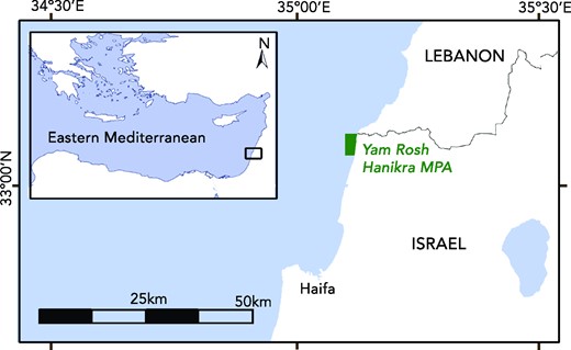
Location of study site. Yam Rosh Hanikra MPA is marked by a green polygon.
Study design
We documented fish communities using three methods: UVC, acoustic surveys, and TDS. We focused on a continuous rocky reef, stretching in parallel to the shore and ranging 5–12 m in depth (Figure 1 and Figure SM1 in the Supplementary Material). Sampling took place along the rocky reef, from 4 km inside the MPA up to 6 km in fished areas.
Underwater visual census (UVC)
UVC is a visual, non-destructive method, providing individual-level data. UVCs in Yam Rosh Hanikra were conducted as part of the Israeli MPA monitoring program led by the Israel Nature and Park Authority (Frid et al., 2021). Surveys were carried out during the spring and fall of 2015, 2017, 2019, and 2021 (eight campaigns in total). To compare fish communities from similar habitat and depth range between the different methods, only data from the medium depth (9.1–17.9 m) was included in this study (Figure 2a). In each site, two scientific SCUBA divers performed 2–4 replicate belt transects (25 long, 6 m wide;3 m on each side of the transect line), resulting in a survey area of 150 m2. Divers recorded the fish species, abundance, and total length (TL) of the entire benthic and benthic-pelagic fish community (excluding cryptic species) up to ∼3 m above the seabed. Prior to the surveys, the divers performed a size-calibration training dive, visually estimating the TL of plastic fish. Mean error for TL estimation was 15% ± 2% (Supplementary Material; Figure SM2). Fish TL were converted into biomass using the length-weight formula:
where W is the fish weight in grams, L is the fish TL in centimeters, and a and b are species-specific parameters obtained from FishBase (Froese and Pauly, 2022). Fish weights were then multiplied by the abundance and summed up to give the total biomass within a transect. We took the data obtained by the more experienced surveyors from each survey team for the analysis. The final UVC dataset for analysis included 143 transects from 50 different locations, extending 4 km inside the MPA and 4 km in fished areas (however, most data reached only 2 km into the fished area).
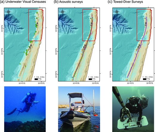
Sampling methods used in this study (a) UVC, (b) Acoustic surveys, (c) TDS. For each method, the top panels show a map with sampling locations/routes (colored diamonds/lines) relative to the MPA borders (red polygons). The bottom panels illustrate typical fieldwork.
Acoustic surveys
Acoustic surveys are a non-intrusive and non-destructive method to study fish populations in their natural habitat using active sound waves (Simmonds and MacLennan, 2005). The acoustic surveys were performed using a Simrad EK80 echosounder system equipped with a wide-band transceiver (WBT) tube and a split-beam circular transducer ES70-7c (Figure 2b). The echosounder was operated in a frequency modulated (FM) mode, emitting wideband “chirp” signals covering 45–90 kHz (nominal frequency 70 kHz). The downward-facing transducer was positioned 0.5 m below the water surface. The nominal half-power (3 dB) beamwidth corresponds to 7°. The pulse duration and ping interval were 0.512 ms and 0.4 s, respectively. The echosounder was calibrated with the standard sphere method using a tungsten carbide sphere of 38.1 mm (Demer et al., 2015). To ensure a reliable representation of fish distribution in the survey area, we used the formula for the degree of coverage, Λ (Aglen, 1989):
where D is the cruise track length, A is the size of the survey area, and for adequate coverage Λ should be ≥ 6. The total size of the rocky reef in the defined study area was 32 km2, requiring us to cover ≥ 34 km per survey. The rocky reef was very narrow, with different habitats on each side (sand on its eastern side or deep canyon on its western side, Figure 2), which limited our ability to perform a classic zig-zag survey. Thus, we designed each survey as multiple continuous linear transects along the east side of the reef and increased the overall sampling effort. Each linear transect (i.e. sampling unit), extended over ∼10 km; 4 km inside the MPA and 6 km in fished areas. Overall, we performed 23 acoustic transects (Supplementary Material; Table SM1), covering a cumulative distance of ∼230 km which ensured a good cover of the study area. The acoustic surveys were carried out during the spring and fall of 2020–2021, during daytime with wave height <0.4 m. Boat speed throughout the surveys was <4 knots.
Acoustic data processing. The raw files of the acoustic data were processed using Echoview 9 software (Echoview Pty Ltd, Hobart, Australia), following the standard operation procedure (Parker-Stetter et al., 2009), to exclude irrelevant/unreliable data (e.g. signals from the seabed, echoes of bubbles, noise near the transducer) and detect the echoes from single targets. Following these stages, only data from 1 m beneath the water surface to 0.5 m above the bottom were used for analysis. To examine the spatial changes, each acoustic recording was divided into 100 m distance intervals, to serve as the elementary sampling distance units (ESDUs) for integration, resulting in a total of 2 574 ESDUs. Acoustic variables for analysis were computed at the center frequency of the band (67.5 kHz) from the obtained wideband acoustic data following the procedure described in Appendix 1. For each ESDU, we produced the mean volume backscattering strength (Sv; dB re 1 m−1) and the nautical area scattering coefficient (NASC, m2 nmi−2). From the single target echoes, which represents acoustic size of individual targets (i.e fish), we produced the target strength (TS; dB re 1 m2) frequency distribution in each ESDU (from −60 to −20 dB, in 1 dB bins). To discern fish from smaller targets, we applied minimum thresholds of −66 dB for Sv and −60 dB for TS (TS = −60 dB corresponds to targets of ∼1.6 cm TL). We used the NASC, which represents the total backscattered energy from fish per area, as a measure of acoustic biomass. To estimate fish density, we used mean Sv and mean TS following the conventional echo integration method (Winfield et al., 2011). For easier comparison with other methods, we also calculated biomass using the TS frequency distribution in each ESDU (Yurista et al., 2014). As none of the main species observed in this study have TS-length conversion coefficients, we used the Love's multispecies TS-length equation (Love, 1971) and general constants for the L-W equation (Froese, 2006). Full description of the methods is presented in the section "Appendix 2". While acoustic biomass estimates are more comparable to the other methods, NASC relies on fewer assumptions and is computed directly by the Echoview software.
Towed-diver survey (TDS)
TDS enable SCUBA divers to visually document a large continuous seascape while towed to a slow-moving boat using a “manta board” (Figure 2c) (Richards et al., 2011). We used the TDS method in parallel to an acoustic survey, extending 4 km within the MPA and 6 km outside the MPA. The ∼10 km transect route was divided into five sections of ∼2 km and each section was surveyed by a different pair of divers. Each diving pair consisted of a fish surveyor and a habitat surveyor. The fish surveyor documented fish continuously within 2.5 m on each side of the surveyor and 3 m above the seabed. The surveyor focused his observations on fish schools (>10 individuals) and large bodied fish (>15 cm), documenting their species, TL, and number of individuals. To simplify the survey, two similar invasive herbivorous fish, Siganus rivulatus and Siganus luridus, were assigned to the genus level (e.g Siganus spp.) and two small-bodied local reef fish, Thalassoma pavo and Coris julis, were excluded from the survey. The habitat surveyor visually evaluated the complexity of the habitat each minute using three metrics: (1) habitat type (sand, gravel, rock), (2) habitat complexity on a scale from 0 to 5, based on Polunin and Roberts, 1993), (3) presence of special rock formations (e.g pinnacle, crack, gorge, wall, or overhang; more than one feature could be recorded in a location). The habitat type was converted into numerical values (sand = 1, gravel = 2, rock = 3) and added to the complexity estimate and the number of special rock features to give an index of total habitat complexity.
The visual records of fish were converted into biomass in the same procedure described for the UVC (section 2.3) and georeferenced using time synchronization with the boat GPS track. Data was then integrated into 50 m intervals, the approximate distance traveled by the boat every minute during the survey, giving an estimation of fish biomass in 250 m2.
Environmental data
For each sampling location/ESDU, we calculated the distance (m) from the south border of the MPA, with negative values representing positions inside the MPA and positive values representing positions outside the MPA. We calculated two complexity indices based on a high-resolution bathymetric map of the study area (horizontal resolution of 4 m and vertical resolution of 10 cm): (1) Slope-calculated based on each pixel's eight neighbouring pixels. (2) Bathymetric position index (BPI, Walbridge et al., 2018), which quantifies depth relative to the overall seascape (mean elevation in a ring with a 2 m inner radius and 50 m outer radius). We tested both the original BPI values (positive and negative values) and the absolute BPI values as predictors in the models (see below), but since there was no difference in the results we used the original values.
Fish characteristics
We examined whether fish characteristics affect the spatial patterns of fish biomass across the MPA border. We used the UVC and TDS datasets and examined: (1) fish size-estimated directly from the visual observations. We additionally estimated two species-level indices: (2) Commercial value-species were classified as either “commercial” or “non-commercial” based on the index of species price category and commercial importance obtained from FishBase (Froese and Pauly, 2022) as well as personal knowledge of the local demand. (3) Fish origin-species were classified as either “indigenous species” (IS) or as “non-indigenous species” (NIS).
Statistical analysis
Spatial patterns.The spatial patterns of fish were modelled using general additive models (GAMs) from the “mgcv” R package (Wood, 2017), which allows to describe non-linear patterns. For all three datasets, we constructed a basic model with distance from the MPA border as a continuous predictor and the relevant response variable (NASC in the acoustic dataset and biomass in the visual datasets). For each method, we included the appropriate random effects: (1) UVC-campaign (8 levels), observer ID (15 levels), (2) acoustic surveys-survey ID (4 levels), (3) TDS-observer ID (2 levels) (Supplementary Material; Table SM2). These random effects were used in all subsequent models. For smoothing of the main predictor (i.e distance from MPA border), we used a thin plate spline (TPS, bs = “tp”). We either log10 transformed the response variable or used the raw values, depending on model fit and the fit to model assumptions (examined on the residuals using the “gam.check” function). For the acoustic data, values of zero were replaced by a small positive number (10−8). The number of basis functions for the GAM smoothing (k values) in each model was adjusted for minimal wiggliness while adhering to model assumption. For all models we applied a gaussian distribution family. We evaluated the entire model, by comparing the basic models to reduced models containing only random effects, based on Akaike information criterion (AIC) and deviance explained (DE). We further examined the effect of environmental factors by including water depth and habitat complexity as fixed effects in the models. For the TDS data we used the visual complexity index, and for the UVC and acoustic data we used slope and BPI. These models were compared to the basic model. For the visual datasets (UVC and TDS), we also tested the effect of fish characteristics on the spatial pattern of fish biomass using the “by” argument in the GAMs The effect of fish size (smaller or larger than 15 cm) and fish origin (IS/NIS) were tested on reduced datasets, containing only the commercial species. A summary table with model formulations is presented in the Supplementary Material (Table SM2).
We estimated the distance (on the X axis) and magnitude (on the Y axis) of edge effects and spillover from the spatial patterns obtained by the GAM models. Edge effect distance was measured as the distance from where the point of highest biomass within the MPA starts to decrease to the MPA border. For spillover, the distance was measured as the distance from the border to the point of lowest biomass outside the MPA. The magnitude of these processes was estimated as the difference in biomass between (1) maximal biomass inside the MPA and the biomass at the MPA border (edge effect), and (2) biomass at the MPA border and the minimal biomass outside the MPA (spillover).
Sensitivity analysis for UVC sample size. We tested whether the clear spatial pattern obtained by UVC is a result of the large sampling effort (n = 143). For this, we selected n random transects (n = 5, 15, 30, 60, 120) from the full dataset, fitted a linear model of the biomass against distance from the MPA border, recorded the slopes, and repeated the procedure 100 times. All statistical analyses were performed in the R environment version 3.6.1 (R Core Team, 2022).
Results
The effect of Yam Rosh Hanikra MPA using the traditional in/out approach
We first compared biomass estimates in the traditional dichotomous approach. When looking at the overall MPA effect (fish biomass inside versus outside the MPA), the difference was strongest in the UVC data and weakest in the acoustic data (gray shaded columns, Table 1). Nevertheless, these differences between inside and outside MPA were generally non-significant for all methods (Table 1). Mean biomass estimates using the visual methods, UVC and TDS, were high in the MPA core (−4–−2 km), decreased close to the border (−2–0 km) and were lowest in the fished areas close to the MPA border (0–2 km). For both visual methods, biomass in the MPA core was ∼200% higher than in the adjacent fished areas. For the acoustic data, biomass in the MPA core was ∼100% higher than in the border area and the adjacent fished areas. In the TDS and acoustic data, biomass estimates in distant fished areas (4–6 km) exceeded the biomass estimates in the MPA core. Biomass estimates obtained with the UVC surveys were 3–4 times higher than the TDS estimates, and the biomass estimates using the acoustic method were an order of magnitude lower than those obtained by both visual methods (Table 1).
Mean biomass estimates (± SD) for UVC, TDS and acoustic surveys integrated over the entire MPA/Fished areas (grey columns) and in 2 km intervals (white columns). To allow comparison, all biomass estimates were converted to units of g/m3.
| Method | MPA | Fished areas | |||||
|---|---|---|---|---|---|---|---|
| Total (−4– 0 km) | Core (−4–−2 km) | Border (−2–0 km) | Adjacent (0–2 km) | Medium (2–4 km) | Far (4–6 km) | Total (0–6 km) | |
| UVC | 15.78 ± 17.92 | 16.76 ± 19.63 | 11.78 ± 6.92 | 5.89 ± 5.77 | 6.5 ± 5.89 | – | 5.88 ± 5.62 |
| TDS | 3.54 ± 4.37 | 3.94 ± 4.58 | 3.18 ± 4.2 | 1.28 ± 1.63 | 2.05 ± 2.32 | 5 ± 7.5 | 2.71 ± 4.61 |
| Acoustic surveys | 0.32 ± 2.31 | 0.45 ± 3.19 | 0.2 ± 1.1 | 0.22 ± 1.74 | 0.88 ± 9.4 | 0.82 ± 7.48 | 0.61 ± 6.82 |
In the visual methods (UVC and TDS), fish identity and size are recorded, allowing us to identify species that benefit from MPA protection and explore the target species captured by each method (Figure 3). The herbivorous, non-indigenous, schooling fish Siganus spp. (S. luridus and S. rivulatus) composed 75% and 72% of the total biomass in the TDS data, compared with only 27% and 33% of the total biomass in the UVC data (MPA vs. fished areas, respectively). In both methods, the proportional biomass of Siganus spp. was relatively similar inside and outside the MPA.

Comparison of fish community composition between Yam Rosh Hanikra MPA and the surrounding fished areas as obtained by UVC (left panel) and TDS (right panel). The Y axis is the relative biomass (%) of each species from the total biomass over the entire dataset and the X axis denotes the location (MPA/Fished). Only species that comprise more than 1% of the total biomass are presented in the graphs.
The proportional biomass of three species of indigenous groupers with high commercial value, Epinephelus marginatus, Epinephelus costae, and Mycteroperca rubra, was higher inside the MPA (43% and 9% for UVC and TDS, respectively) compared to fished areas (11% and 2%). In both methods, the biomass of Chromis chromis, a small non-commercial schooling fish, was higher in fished areas compared to inside the MPA, with relatively higher proportions in the UVC data (UVC: 16% and 7%, TDS: 7% and 3%, fished areas vs. MPA, respectively). Taeniura grabata, a large indigenous Batoid, presented an opposite trend with higher biomass inside the MPA compared to fished areas in both methods, and with relatively higher proportions in the TDS data (UVC: 4% and 1%; TDS: 7% and 4%, MPA versus fished areas, respectively). Overall, this small group of species (two species of Siganus spp., three species of groupers, C. chromis, and T. grabata) composed 61% and 81% of the total fish biomass in the UVC data and 85% and 94% in the TDS data (fished areas versus MPA, respectively).
Continuous spatial patterns across Yam Rosh Hanikra MPA border
The continuous spatial patterns of fish as a function of distance from the Yam Rosh Hanikra MPA border, obtained using three different methods, are presented in Figure 4 (results for models with distance as the main predictor compared with reduced models including only random effects: Figure 4a-UVC: ΔAIC = 30.6, DE = 32.3%, p-value distance <0.001; Figure 4b-Acoustic survey based on NASC: ΔAIC = 25.52, DE = 49%, p-value distance <0.001; Figure 4c-TDS: ΔAIC = 4.68, DE = 5.51%, p-value distance <0.05). Inside the MPA, we observed an almost linear decrease in fish biomass/NASC in log10 scale in all three methods, with highest values recorded in the northernmost part of the MPA, decreasing across the MPA border (Figure 4). This is consistent with an edge effect that extends to the innermost part of the MPA. Modelling the spatial patterns of fish based on acoustic density and biomass produced similar patterns to NASC Supplementary Material; Figure SM3).

Continuous spatial patterns of fish communities across Yam Rosh Hanikra MPA borders based on data obtained using three different methods: (a, d) UVC, (b, e) Acoustic surveys, and (c, f) TDS. Top panels are results for GAMs with distance as a sole predictor, and bottom panels are model results with distance, water depth, and habitat complexity as predictors. The Y axes are the total fish biomass (log10 transformed) per area For UVC and TDS, and NASC (log10 transformed) for the acoustic surveys. The X axes are distance (km) from the MPA border and dashed vertical lines represent the MPA border. Shaded areas around the model curves denote 95% confidence intervals.
Outside the MPA, the spatial patterns were also similar among methods with slight changes. Biomass in the UVC data continued to decrease up to 2 km from the border, and then showed a slight increase from 2 to 4 km (Figure 4a). Both the TDS and acoustic data displayed a similar pattern to the UVC data (within the same range), but also detected an increase in biomass from ∼2–2.5 km to 6 km south of the MPA border (Figure 4b and c). For the acoustic data, when we increased the “wiggliness” parameter of the GAM; e.g. when we increased the number of basis functions to k = 10, we detected additional peaks both within and outside the MPA (Supplementary Material; Figure SM4).
The spatial pattern of the three methods differed when incorporating water depth and habitat complexity indices into the models. For the UVC data, incorporating depth or complexity did not improve the models (results for models with distance, water depth and habitat complexity indices as main predictors compared with reduced models including only distance: Figure 4d, ΔAIC = −4.6, DE = 31.6%, p-values: distance <0.001, depth = 0.77, slope = 0.46, BPI = 0.48). In the acoustic data, incorporating depth to the model caused a disappearance of the peak in NASC values far from the MPA border, yet distance remained significant (Figure 4e, ΔAIC = 83.98 compared to a model with distance only, DE = 50.7%, p-values: distance <0.05, depth <0.001, slope = 0.85 BPI = 0.07). In the TDS data, adding the visual complexity index to the model explained most of the variability in the data. Distance was no longer a significant variable and the spatial pattern almost disappeared (Figure 4f; ΔAIC = 30.4 compared to a model with distance only, DE = 12.9%, p-values: distance = 0.28, depth = 0.93, visual complexity <0.001).
The effect of fish characteristics
We next examined how different fish characteristics affect the patterns across the MPA border. We found that the dominant pattern of high biomass in the MPA core, decreasing towards the border and fished areas, is mainly associated with species of commercial value (results for models including commercial value compared with reduced models including only distance, depth, and habitat complexity: Figure 5a-UVC: ΔAIC = 83.73, DE = 42.9%, p-value commercial <0.001; Figure 5b-TDS: ΔAIC = 43.95, DE = 27.6%, p-value commercial <0.001). Testing the effect of fish size, we found that the pattern of decreased biomass across the MPA border was influenced mostly by large-bodied individuals (TL >15 cm, Figure 5c-UVC: ΔAIC = 40.22, DE = 29.2%, p-value fish size <0.001; Figure 5d-TDS; ΔAIC = 1.53, DE = 17.7%, p-value fish size <0.01). Examining the effect of fish origin (IS: indigenous species, vs. NIS: non-indigenous species), we found different patterns for models based on different methods. While the UVC data showed that the decrease in biomass across the MPA border is associated with indigenous species, the TDS data indicate that the decrease in biomass is mostly associated with non-indigenous species (Figure 5e-UVC: ΔAIC = 8.83, DE = 30.5%, p-value fish origin <0.1; Figure 5f-TDS: ΔAIC = 14.28, DE = 22.7%, p-value fish origin <0.001).
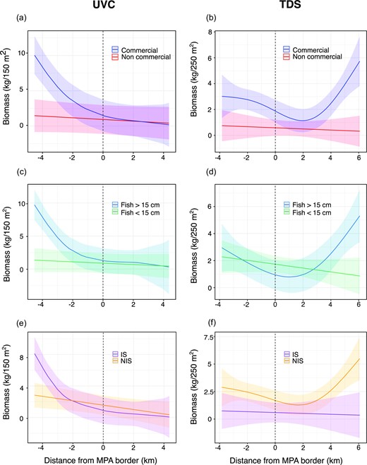
The effect of fish characteristics on the spatial patterns of fish biomass across Yam Rosh Hanikra MPA border. (a, b) fish commercial value (commercial/non-commercial), (c, d) fish size (< 15 < cm), and (e, f) fish origin (IS: indigenous species, NIS: non-indigenous species). Left panels are based on UVC data and right panels are based on TDS data. The Y axes are fish biomass per area and the X axes are distance (km) from the MPA border. Dashed vertical lines represent the MPA border. Response variables are shown on the linear (non-log-transformed) scale for visualization purposes. Shaded areas around the model curves denote 95% confidence intervals.
Based on the species composition analysis, we also constructed models for the main species in the datasets, i.e groupers and Siganus spp.. This analysis approved that the spatial patterns based on the TDS data largely follow the pattern obtained for the Siganus spp. alone, and that the patterns based on the UVC data resemble the spatial pattern obtained for groupers alone (Supplementary Material; Figure SM5).
Comparing methods in terms of sampling effort
To evaluate our ability to detect patterns in relation to sampling effort, we compared the sampling days, manpower required, area and volume sampled, and estimated costs per survey day and area sampled (Table 2). Both the area and volume of water sampled by the acoustic method were an order of magnitude larger than those sampled with the UVC, with the same amount of sampling days and a quarter of the people-days. The area and volume covered by one TDS were twice as large as all 143 UVCs transects, with a quarter of the sampling days and fifth of the people-days. Overall, UVC is the most costly method per area surveyed, followed by the acoustic method, with TDS being the least costly.
Summary of the sampling effort performed in each of the methods in the study.
| Parameter/Method | UVC | TDS | Acoustic survey |
|---|---|---|---|
| Sampling days | 8 | 2 | 8 |
| People days | 64 | 10 | 16 |
| Number of transects | 143 | 1 | 23 |
| Estimated area sampled | 21 450 m2 | 50 000 m2 | 218 000 m2 |
| Estimated volume sampled | 64 350 m3 | 150 000 m3 | 1 138 500 m3 |
| Estimated cost per survey day ($) | 9050 | 8050 | 10 500 |
| Estimated cost per m2 sampled ($) | 5 | 0.32 | 0.37 |
UVC sample size
We also tested whether the clear spatial pattern obtained by the UVC is a result of the high number of transects (n = 143), and whether reducing the sampling effort can produce similar results. The results demonstrate that even with only five transects, a clear pattern of decreasing biomass with distance from the MPA border is observed (Figure 6). Nonetheless, increasing the sampling effort produced higher intercept values and steeper slopes.
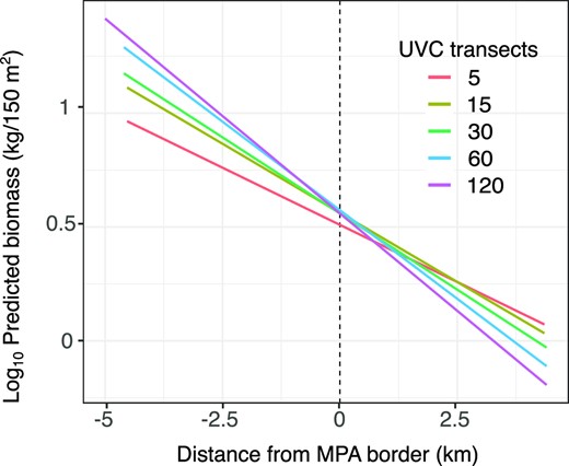
Predicted fish biomass with distance from the MPA border based on different UVC sample sizes. The Y axis is the log10 transformed predicted fish biomass (kg) and the X axis is distance from the MPA border (km). The different colors represent the average results for different numbers of transects based on 100 repetitions.
Discussion
Our study examined the effect of the Yam Rosh Hanikra no-take MPA on fishes using both a dichotomous approach (in/out), and a continuous approach, examining the spatial patterns across the MPA into fished areas as far as 6 km from the MPA border. We used three different methods and found support for the prevalence of strong edge effects and minor spillover even in a well enforced no-take MPA. These findings highlight the need for continuous sampling in the spatial domain to reveal such patterns.
The effect of Yam Rosh Hanikra MPA using the traditional in/out approach
We consistently found higher biomass values in the MPA core (−4–−2 km) relative to adjacent fished areas (0–2 km). These trends were captured by all three methods, although these differences were non-significant (Table 1). The non-significant differences reflect the large spatial variability in biomass estimates. Spatial sampling can potentially overcome this challenge, and reveal areas of high and low biomass both within and outside the MPA. In terms of species compositions, the benefits of MPA protection were mainly expressed by the increase of the commercial grouper species relative to the fished areas (Figure 3).
Continuous spatial patterns of fishes across Yam Rosh Hanikra MPA border
The spatial patterns presented a general trend of high biomass in the northernmost part of the MPA, decreasing towards and across the MPA southern border, and lowest in the adjacent fished areas (Figure 4). These results indicate that the real core of Yam Rosh Hanikra MPA, the area with highest biomass, is not in the centre of the MPA, but rather in the northernmost area. When considering the restricted border area between Israel and Lebanon (Figure 1), which prohibits human activity, this is actually the effective centre of the non-fished areas.
We found a dramatic decrease in biomass/NASC values around the MPA border area across all survey methods (Figure 4). These patterns imply that the MPA may be experiencing edge effects (Ohayon et al., 2021), most likely as a result of intensive fishing along the MPA border, i.e. fishing the line (Kellner et al., 2007). Indeed, data on fishing enforcement events indicate a high density of fishing activity along the southern border of the MPA (Supplementary Material; Figure SM6). The spatial pattern of edge effect reflects a reduction of ∼50% in biomass along 4 km, from the northernmost part of the MPA to its southern border.
Outside the MPA, the biomass pattern in the UVC and acoustic data continued to decrease up to 2–3 km outside the border, reflecting a minor pattern of spillover. For the TDS data, there is no apparent pattern of spillover. The inability to detect significant patterns of spillover may be a result of intensive fishing, which rapidly depletes exported fish along the border, together with an absence of a partially protected area (buffer zone; Di Lorenzo et al., 2020) around Yam Rosh Hanikra MPA.
We detected a surprising pattern of high biomass 6 km from the MPA border using the acoustic surveys and TDS. This can be a result of several scenarios: (1) Increased biomass unrelated to fishing, driven, for example, by habitat features. In support, we note that this pattern mostly disappears for the acoustic and TDS data after accounting for habitat complexity. (2) Higher fishing activity closer to the MPA border, leading to an increase in fish biomass farther away from the MPA where fishing pressure decreases (Hilborn, 2018). (3) Differential response of species to protection and fishing, e.g. decrease in groupers leading to predator release far from the MPA (e.g. for Siganus spp. see below). Further surveys in this area can determine which of the scenarios is more likely to create this pattern.
Habitat structure is an important factor shaping fish distribution and abundances (Gratwicke and Speight, 2005; Lazarus and Belmaker, 2021). In the acoustic and TDS data, accounting for habitat complexity reduced the effect of distance. A possible explanation is that for species that are better recorded using these methods, such as C. chromis and Siganus spp., habitat complexity may play a more substantial role than MPA protection. Specifically, C. chromis schools are often associated with small-scale rock features (pinnacles, walls, cracks, etc.). These features may be better represented in the visual assessments of complexity than in the BPI index, explaining more variability in fish biomass when using TDS data. We did not find an effect of habitat complexity on the spatial pattern of biomass using the UVC method. It is possible that the resolution of the BPI index is too coarse for explaining fish distribution at the scale of UVC. Alternatively, for groupers, which are highly targeted by fishing, the MPA effect could be stronger than the effect of habitat complexity (Di Franco et al., 2021; Ziegler et al., 2022).
The effect of fish characteristics
We were able to confirm the effectiveness of MPAs in protecting species with commercial value, specifically large individuals when using UVC and TDS (Figure 5). However, we found that the relative proportions of species recorded by each method is different (Figure 3). UVC recorded large and commercially valuable grouper species better than the TDS.
Groupers are iconic species for fishers and are extremely favoured by spatial protection (Hackradt et al., 2014). In the UVC data, the sharp increase in biomass in the MPA core is mainly related to the large bodied, indigenous groupers, while in the TDS data the pattern is mainly associated with the smaller non-indigenous Siganus spp. (Figure SM5). Siganus spp. have a commercial potential, but in practice they are of low demand and are not heavily fished. These differences in target species can explain the weaker MPA effect and lower biomass observed using the TDS method.
Highly enforced MPAs have been suggested as a tool to combat biological invasions (Giakoumi and Pey, 2017). According to the biotic resistance hypothesis, one can expect the higher biomass of groupers to be associated with reduced biomass of NIS, especially their prey Siganus spp. (Shapiro Goldberg et al., 2021). While we found that grouper biomass reached a maximum in the MPA core (Figure SM5a), we did not see evidence for a parallel decrease in Siganus spp. biomass (Figure SM5b). This finding is consistent with previous studies, which did not find clear evidence for biotic resistance (Giakoumi et al., 2018). Nonetheless, we found a gradual increase in biomass of Siganus spp. with increasing distance from the MPA border, which may be explained by a combination of a decrease in the fishing pressure (Figure SM6) and lower predation by groupers.
The effect of the survey method
All three methods detected a general MPA effect (higher biomass rates in the MPA core relative to adjacent fished areas, Table 1), which is surprising given that each method captures different facets of the fish community. Although UVC is the most common method for MPAs monitoring, it is not usually perceived as a method for continuous sampling. Our results show that UVC actually presented clear and consistent spatial patterns, associated mainly with grouper species. We demonstrate that even with much fewer sampling locations, a clear gradient of decreasing biomass across the MPA border can be detected (Figure 6). Increasing the sample size, however, produced steeper slopes, which may indicate a larger edge effect and a lower spillover distance. Following these results, we suggest that UVC should be more frequently used as a tool for spatial assessment of MPAs performance. This can be achieved by moving away from a simplistic in/out sampling design, to spreading the sampling sites more evenly over larger areas and analyzing the data continuously.
TDS is a much faster and cheaper method than UVC (Table 2), yet it captures a much smaller subset of species. This means that the ability to reveal patterns is prone to ecological contingencies associated with the identity of particular species. For example, for the TDS data, the increase in biomass in distant fished areas is mostly related to the non-indigenous, large bodied commercial Siganus spp. (Figure SM5b). The use of TDS for MPA monitoring may be improved by pre-defining the main target species for surveys.
The acoustic method allowed us to cover large areas inside and outside the MPA efficiently. However, the biomass estimates were an order of magnitude lower than the visual methods (Table 1). This result can be related to both ecological and methodological reasons. Ecologically, acoustic methods focus on pelagic and benthic-pelagic species, as it is limited in differentiating fish from the seafloor (the “acoustic dead zone”) (Ona and Mitson, 1996). The multiple peaks revealed by the acoustic method when we increased the model wiggliness (e.g. k = 10, Figure SM4) may also reflect the more stochastic response of mobile pelagic and benthic-pelagic fish species to MPA protection (Kramer and Chapman, 1999). Methodological limitations may also impact the efficiency of the acoustic method. At shallow depths, the echosounder beam width is narrow (0.6–1.2 m beam diameter for 5–10 m water depth), reducing the ability to capture rare events of high biomass, such as large schools of pelagic mobile species. A recent study from an MPA in Senegal also highlighted the challenges of monitoring fish in shallow waters using acoustic methods (Béhagle et al., 2018). While acoustic methods have the advantage of covering large areas in short-time, they may be less effective in shallow areas and in multi-species assemblages.
Summarizing the comparison among methods, we find that all three methods captured the increase in fish biomass/NASC within the MPA core, gradually decreasing across the MPA borders. We recommend improving the UVC sampling design to provide better spatial coverage by moving away from binary in/out sampling and increasing the spatial extent and evenness of samples at the expense of more repetitions within each site. At the same time, our study highlights the advantages of acoustic and TDS methods in discovering biomass “hot spots.” Thus, the quick and cost-effective TDS can serve as a complementary method to survey specific target species. With most of the existing MPAs covering shallow coastal areas, the advantages of the acoustic method relative to other methods is reduced. Nonetheless, acoustic methods have a potential for spatial monitoring of pelagic fish in deep-water MPAs. Additional visual methods not tested here, such as baited remote underwater video (BRUV) or autonomous underwater vehicles (AUV), can be used both as monitoring tools and as ground truthing for the acoustic methods (Ferrari et al., 2018; La Manna et al., 2021). Developing and testing new methods for spatial evaluation of MPAs is essential to provide early warning for degradation of fish biomass within MPAs, and to understand the temporal trends in the magnitude of spillover.
Caveats
When comparing among methods, we acknowledge the differences in the exact locations surveyed. For example, acoustic and TDS surveys were conducted along the east side of the rocky reef, while most UVC sites were located on its west side (Figure 2). The UVC locations were part of a long term monitoring program (Frid et al., 2021), and hence could not be modified. Nevertheless, the similar patterns obtained using the three methods increase the robustness of our findings.
Each of the methods used in this study may produce method-specific biases. In the visual methods, surveyor's experiences may impact biomass estimations (Edgar et al., 2004). In addition, fish may display divers or vessel avoidance behaviour (De Robertis and Handegard, 2013), underestimating actual fish biomass. However, since we used the same sampling protocols inside the MPA and in fished areas, these biases should not affect the observed spatial patterns. Of larger concern are biases that may impact fish differentially within and outside the MPAs. For example, fish in fished areas may avoid divers or boat noises to a larger degree than fish inside the MPA (Diaz Pauli and Sih, 2017). Controlling for these biases is beyond the scope of this study and further research is needed to evaluate their effect on patterns of fish biomass.
In the acoustic data analysis, we used generalized conversion rates (Appendix 2) to translate the acoustic signals into biomass, which may lead to under or overestimations of biomass depending on the fish community composition. We tested the sensitivity of acoustic estimates by comparing TS-length and TS-weight relationships for two species similar to the major species found in this study: a grouper (Epinephelus awoara) and Siganus (Siganus canaliculatus). The TS-length and TS-weight relationships show that for the same TS level, the grouper has larger length and weight compared with the Siganus (Supplementary Material; Figure SM7). In this study, the visual methods suggest that the proportions of Siganus spp. were similar in and out the MPA, while groupers were more dominant in the MPA (Figure 3). These results suggest that the pattern of higher acoustic biomass/NASC in the MPA may even underestimate the true contrast between the MPA and fished areas.
Conclusions
Much attention is dedicated to improving MPAs spatial planning in terms of size, shape, zoning, and connectivity (Balbar and Metaxas, 2019; Fox et al., 2019). However, the spatial aspects of MPAs performance and the appropriate methods to examine them are still understudied. In this study, we documented the spatial patterns of fishes across MPA borders continuously, using three non-destructive methods. We found evidence for strong edge effects in Yam Rosh Hankira no-take MPA, as well as evidence for a pattern consistent with fishing the line. These patterns emphasize the risks overfishing pose even to well enforced no-take MPAs, and suggest that additional measures such as the implementation of buffer areas is needed to assure the long-term sustainability of MPAs (Di Lorenzo et al., 2020; Ohayon et al., 2021). At the same time, the observed patterns stress the importance of continuous spatial monitoring of MPAs and exploited fish populations around them.
Acknowledgement
We would like to thank S. Selingre, M. Lazarus, Y. Buba, S. Chaikin, R. Dega, T. Gavrieli and O. Hepner for field assistance. We thank D. Shapiro-Goldberg for reviewing the manuscript.
Funding
This research was partially supported by the Israel Nature and Parks Authority.
Authors contributions
S.O. designed the study, collected the data, performed the data analysis and wrote the original manuscript. H.H. assisted with acoustic data collection, analysis, and writing of sections relevant to the acoustics. S.M. designed the acoustic system platform and participated in the field work. I.O. conceptualized the study and reviewed the manuscript. R.Y. provided access to the Bioblitz UVC data. T.M. conceptualized the study, reviewed the manuscript and assisted with improving its structure. M.K. performed habitat complexity analysis and created the maps. J.B. conceptualized the study, supervised the work, assisted with data analysis and wrote the original manuscript.
Conflict of interest statement
The authors declare no conflict of interest.
Data availability statement
The UVC data is available on Biotime (https://biotime.st-andrews.ac.uk/). The acoustics and TDS data will be made available by the authors to any qualified researcher upon request.
