


Abstract
Human intervention and climate change jointly influence the functions and dynamics of marine ecosystems. Studying the impacts of human and climate on ecosystem dynamics is challenging. Unlike experimental studies, research on natural systems is not amendable at the scale of time, space, and biology. With confounding factors well balanced for two adjacent subtropical estuaries except urbanized disturbances, we conducted ecosystem modelling using indirect reasoning by exclusion to quantify the relative impacts of human disruption on estuarine ecosystems under climate variability. One major finding of this study is that the human intervention tends to magnify species fluctuations, complicate the species interaction network, and enhance species interaction strength combined with disclosed downscaling climate effects (indexed as North Atlantic Oscillation and Atlantic Multi-decadal Oscillation) on estuarine hydrology and biological communities. In addition, functional groups appeared to respond more diversely to external forcing in company with human interventions. While human perturbation was shown to destabilize the estuarine ecosystems, making them vulnerable to environmental variability under climate change, buffering effects of species diversity and trophic interaction tend to underpin the ecosystem functions. The findings of this study contribute to the holistic assessment and strategic management of estuarine ecosystems subjected to human and natural disturbances in the face of climate change.
Introduction
Human activities and changing climate jointly affect marine ecosystems (Harley et al., 2006; Cloern et al., 2016). Increasing evidence indicates that coastal marine ecosystems have been experiencing extensive man-made alterations (Thrush et al., 2003; Madin et al., 2016), including massive loss and fragmentation of habitats (Jackson et al., 2001), hypoxia and acidification (Rabalais et al., 2001), and land-derived pollution (Lotze et al., 2006). In addition, climate change poses another layer of threat to ecosystem functioning (Hughes et al., 2003), as demonstrated in numerous ecosystem collapses (Hoegh-Guldberg et al., 2017; Canadell and Jackson, 2021). While the importance of human–climate–ecosystem interactions has been well recognized (Redman, 1999; Levin et al., 2015), assessing the relative impacts of the triad remains inadequate, mainly because studies on natural ecosystems are not amendable compared to experimental studies at the scale of time, space, and biology. Such inherent dilemmas often lead to risks and uncertainties when performing strategic management of sustainable marine ecosystems.
Viewpoints suggest that human activities tend to decouple ecological relationships such as predator–prey (Rodewald et al., 2011) and host–parasite interactions (Wood et al., 2018). The decoupling tends to be exacerbated in subtropical waters such as the northern Gulf of Mexico (GoM) under climate change (Fodrie et al., 2010), companied with northward intrusion of tropical species (Fujiwara et al., 2019). Selecting subtropical estuaries, we attempt to examine the climate–human synergy on ecosystem dynamics and tease out anthropogenic impacts on ecosystem dynamics under climate scenarios. We target on two adjacent estuaries (Galveston Bay and Matagorda Bay, Texas, USA), which share similarities in climatology, hydrography (Engle et al., 2007), and ecology (Fujiwara et al., 2019), yet with distinct urbanization. Specifically, Galveston Bay (the largest estuary in Texas) surrounded by the greater Houston metropolitan area (the fifth most populous in the USA) is highly urbanized and more subject to anthropogenic activities (e.g. wastewater disposal, dredging, shipping, and coastal construction), whereas Matagorda Bay (the second in size to Galveston Bay) within a rural region still remains relatively undeveloped (Brody et al., 2004).
Long-term ecological time series are valuable indicators of dynamic marine ecosystems (Bi et al., 2022). We employ the fisheries-independent survey data collected over 35 years (1984–2018) in Texas estuaries to quantify how climate change in combination with distinct human pressure affects the two estuarine ecosystems. In this study, we apply empirical dynamic modelling (EDM), a nonparametric modelling approach (Sugihara et al., 2012), to overcome the hurdle of capturing ecosystem nonlinearity using traditional statistical models. EDM has shown great potential to forecast nonlinear dynamics and delineate the complexity of the system dynamics (Sugihara and May, 1990; Sugihara, 1994) and has been applied to provide science-based advice in support of fisheries management (Glaser et al., 2014; Ye et al.,2015; Harford et al., 2017; Liu et al., 2012, 2017a). In addition, convergent cross mapping (CCM), an extension of EDM, has been used to identify causal relationships and shared dynamics in marine ecosystems (Deyle et al., 2013; Clark et al., 2015; Kuriyama et al., 2020).
Ecosystem-based management (EBM) highlights the need for a holistic assessment of the status of an ecosystem (Curtin and Prellezo, 2010; Liu et al., 2012, 2014), in which different ecological processes yet often operate at various scales (Hastings, 2010). It is thus interesting to know the scale-based state of ecosystem components across time and space, from species to ecosystems (Nagelkerken and Munday, 2016). By integrating ecosystem components at three hierarchies: species level, functional group level, and ecosystem level, in this study we address a central question in ecology of detecting the mechanisms of driving ecosystem dynamics subjected to the human–climate synergy from a new perspective.
One key effort towards EBM requires knowing the capacity of an ecosystem to withstand or recover from external perturbations, normally referred to as “stability” (Gunderson, 2000; Oliver et al., 2015). Earlier studies have introduced well-defined measures of ecosystem stability such as the scaling relationship between the mean and the variance of abundance or biomass (Doak et al., 1998; Tilman et al., 1998). Herein, we consider the coefficient of variation (CV) of the integrated abundance of functionally similar species to indicate functional group stability. Further, to quantify ecosystem dynamics, we use local Lyapunov stability derived from the time-varying species interaction matrix, which can handle the complexity of non-equilibrium systems (Ushio et al., 2018).
Underlying mechanisms driving ecosystem stability can be diverse. For example, the cascading effects of large-scale climate drivers [e.g. Oceanic Niño Index (ONI), North Atlantic Oscillation (NAO), and Atlantic Multi-decadal Oscillation (AMO)] on local environmental properties (e.g. river discharge, water temperature, and salinity) and further on biotic variability have been well documented in the northwestern GoM (Tolan and Fisher, 2009; Pollack et al., 2011; Fujiwara et al., 2019; Rodriguez-Vera et al., 2019; Tominack et al., 2020). A coupled effect of NAO and AMO has been found to influence the recruitment success of Gulf menhaden (Brevoortia patronus) by changing regional physical and biological processes (Sanchez-Rubio and Perry, 2015). Ecosystem stability has also been empirically linked to biodiversity (Loreau et al., 2001; Hooper et al., 2005), species interaction strength (Navarrete and Berlow, 2006; Tang et al., 2014), and functional group stability (Bell et al., 2014). All of which may exert stabilizing effects to specific ecosystems; however, the knowledge of how these components mechanistically linked remains limited (Hautier et al., 2015). Here, we seek to understand mechanisms contributing to stability in ecosystem functioning under direct and indirect effects of climate change and human disturbance.
The overall aim of this study is to quantify and partition the relative impacts of external perturbations on ecosystem dynamics through performing a “pseudo experiment” on two geographically and ecologically similar estuarine ecosystems but exposed to distinct human activities. Specifically, we apply a heuristic nonlinear modelling approach to analyse fisheries-independent time series (1984–2018) and examine the ecosystem dynamics of the two estuaries. Our hypotheses are: (1) human activities and climate variability impose pressures on local environments that amplify ecosystem vulnerability; while biodiversity and species interaction tend to alleviate these external perturbations and therefore sustain ecosystem functioning; and (2) a less disrupted system may show strong adaptability to external perturbations because of the resilience of its internal functional groups. This study is designed for fully understanding estuarine ecosystems to contribute to the improved knowledge of the underlying mechanisms by which humans act on coastal ecosystems under increasing climate variability.
Methods
Study sites
Galveston Bay and Matagorda Bay in Texas, USA are two of the largest estuarine systems along the northwestern GoM coast (Figure 1). While the two estuaries are geographically adjacent and share similar hydrological features (Table 1, Supplementary Figure S3), the impact from human activities is distinct to differentiate the two systems. Specifically, Galveston Bay surrounded by the greater Houston area has been subjected to intense human activities over decades; whereas Matagorda Bay, second in size to Galveston Bay among the Texas estuaries, is relatively less urbanized and underdeveloped (Brody et al., 2004).
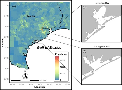
(a) Population density by census tract in Southeast Texas, USA (data from the 2020 decennial US census). (b and c) Maps of Galveston Bay and Matagorda Bay.
Comparisons of characteristics between Galveston Bay and Matagorda Bay.
| Item | The Galveston Bay System | The Matagorda Bay System | Source |
|---|---|---|---|
| Sub-bay | Trinity, Galveston, East, and West Bays | Lavaca, Carancahua, Tres Palacios, and Espiritu Santo Bays | http://www.gulfbase.org/ |
| Surface area | 1 399 km2 | 1 093 km2 | http://www.gulfbase.org/ |
| Drainage area | 63 500 km2 | 109 300 km2 | http://www.gulfbase.org/ |
| Average fresh water inflow | 430 m3/s | 150 m3/s | http://www.gulfbase.org/ |
| Average depth | 2.0 m | 2.0 m | http://www.gulfbase.org/ |
| Average salinity | 11 ppt | 19 ppt | http://www.gulfbase.org/ |
| Coastal wetlands | 1 594 km2 | 348 km2 | http://www.gulfbase.org/ |
| Submerged aquatic vegetation | 73 km2 | 28 km2 | http://www.gulfbase.org/ |
| Tidal height | 0.16 m | 0.12 m | Engle et al.(2007) |
| Rainfall | 112 cm/year | 102 cm/year | Montagna et al.(2007) |
| Commercial finfish harvest | 176 000 kg/year | 59 000 kg/year | Montagna et al.(2007) |
| Commercial shellfish harvest | 4 352 000 kg/year | 2 531 000 kg/year | Montagna et al.(2007) |
| Population | 6.7 million | 147 680 | https://www.census/gov/quickfacts/fact/table/US# |
| Urban development | Heavily developed | Relatively undeveloped | Lester et al.(2002), Brody et al.(2004) |
Data acquisition
Texas Parks and Wildlife Department (TPWD) conducts a long-term standardized fishery-independent monitoring programme to assess the trend of relative abundance and size of finfish and shellfish in Texas estuaries (Martinez-Andrade et al., 2005). Time series of fisheries-independent data (1984–2018) used in this study were collected following stratified randomized sampling design during the biweekly bag seine (13-mm-mesh bag, 1.8-m deep, 18.3-m long) surveys, which include over 10 million individuals of 602 taxa consistently sampled in the two bay systems. Seines were deployed along the shoreline during daylight hours and pulled parallel to the shore for 30.5 m, which covers a total area of 0.03 ha for each haul.
Using Olmstead–Tukey test (Sokal and Rohlf, 1995), we defined dominant species based on the following steps: (1) filter out species with at least 500 records during the period (1984–2018); (2) calculate the log-transformed frequency of occurrence and relative abundance for each species; and (3) use the median calculated from each axis as a cut‐off score and select dominant species above the two cut-off scores. From the frequency-abundance quadrant graph (i.e. Olmstead–Tukey diagram, Figure 2), we extracted 11 dominant species: Atlantic croaker (Micropogonias undulatus), bay anchovy (Anchoa mitchilli), blue crab (Callinectes sapidus), brown shrimp (Farfantepenaeus aztecus), Gulf menhaden (Brevoortia patronus), inland silverside (Menidia beryllina), pinfish (Lagodon rhomboides), spot (Leiostomus xanthurus), striped mullet (Mugil cephalus), white mullet (Mugil curema), and white shrimp (Litopenaeus setiferus). Time series of relative abundance of 11 dominant species in Galveston Bay and Matagorda Bay are shown in Supplementary Figures S1 and S2. Species with ecological equivalence may exhibit similar dynamic features (Liu et al., 2012, 2014) and respond similarly to environmental forcing (Hooper et al., 2005; Loreau and Mazancourt, 2008). Therefore, a particular focus was given to the functional group level within this study, allowing us to study the dynamics of higher-level organizations in response to external forcing. At an ecosystem level, we calculated monthly Shannon–Wiener diversity and richness indices based on the time series of all taxa of fish and invertebrates. Given different sampling efforts between sites and years, the diversity metrics were calibrated using rarefaction curve to extrapolate the true value of diversity (Chao et al., 2014). The rarefaction curve describes the relationship between diversity metrics and the number of samples, and as sample size increases, diversity increases monotonically until reaches asymptote. Applying this method allows us to compare diversity metrics from different sites and years at the same level of effort.
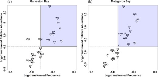
Illustrating the relationship between log-transformed frequency (probability of occurrence/sample) and relative abundance (number of catch/sample) of species in (a) Galveston Bay and (b) Matagorda Bay. The squares show occasional (upper-left), dominant (upper-right), rare (lower-left), and frequent (lower-right) species according to the Olmstead–Tukey diagram. Note that dominant species (n = 11) within the purple square are used in our study. Species names and abbreviations are listed below: Atlantic croaker (AC), bay anchovy (BA), bay whiff (BW), blue crab (BC), brown shrimp (BS), daggerblade grass shrimp (DGS), eastern oyster (EO), Gulf killifish (GK), Gulf menhaden (GM), dardhead catfish (HC), inland silverside (IS), lesser blue crab (LBC), longnose killifish (LK), pinfish (PF), red drum (RD), sand seatrout (SDT), sheepshead minnow (SHM), southern flounder (SF), southern kingfish (SK), spot (SP), spotfin mojarra (SFM), spotted seatrout (SPS), striped mullet (SM), thinstripe hermit crab (THC), white mullet (WM), and white shrimp (WS).
Hydrological time series were compiled from multiple data sources. In-situ water temperature and salinity were measured during the TPWD biweekly bag-seine surveys. In Galveston Bay, the Trinity River provides 55% of total freshwater input (Guthrie et al., 2012), and its river discharge is considered to characterize the inflow of the bay (Buzan et al., 2009). Therefore, the streamflow dataset of Trinity River from a USGS gauge station (# 08066500, Trinity Rv at Romayor) was used as a proxy for the river discharge in Galveston Bay (https://waterdata.usgs.gov/usa/nwis). The majority of inflow of Matagorda Bay comes from the Lavaca River and Tres Palacios River (Kim and Montagna, 2009). The streamflow data for Matagorda Bay were obtained from two USGS gauge stations (# 08164000, Lavaca Rv nr Edna and # 08162600, Tres Palacios Rv nr Midfield, https://waterdata.usgs.gov/usa/nwis).
To include climate variability in the analyses, we considered three climate indices: ONI (https://psl.noaa.gov/data/correlation/oni.data), NAO (https://www.ncdc.noaa.gov/teleconnections/nao/), and AMO (https://climatedataguide.ucar.edu/climate-data/atlantic-multi-decadal-oscillation-amo).
In this study, a period from 1984 to 2018 at a monthly scale for all biotic and abiotic was used throughout time series analyses and EDM. Before the nonlinear modelling, each time series was standardized with a mean of 0 and a standard deviation of 1 for normalization.
Time-lagged coordinate embedding
From a perspective of nonlinearity, complex dynamics evolving through time is governed by an underlying attractor—a geometric object formed by empirical trajectories (Sugihara and May, 1990). A pioneering study has demonstrated that the “shadow” attractor of a state-dependent system can be reconstructed using time-delayed coordinate embedding (Takens, 1981). Simply put, a single time series variable x and its lags can be embedded into an E dimensional phase space (i.e. Xt = [xt,xt−τ,xt−2τ,…,xt−(E−1)τ]) as a topologically equivalent representation of the original state space, where t is the discrete time interval and τ is the time lag (τ = 1). The embedding dimension E is the minimum number of coordinate variables to untangle state trajectories without overlap (Takens, 1981; Sugihara and May, 1990).
Simplex projection
Simplex projection assumes the behaviour of a dynamic system has connections with the recent past (Sugihara and May, 1990). In E-dimensional phase space, the position of the prediction vector (Xt) (i.e. a target point for prediction) in the next time step (Yt+1) can be predicted by first identifying the E + 1 nearest neighbours of Xt and then tracking the position of these neighbours at time t + 1. Here, the E + 1 nearest neighbours are selected based on the Euclidean distances between the prediction vector (Xt) and all library vectors {Xi} (i.e. whole library of points). The forward projection (Yt+1) is the product of the exponentially weighted average of the neighbours at time t + 1 (Xt+1), given by
where the weight for each neighbour vector is computed by |${w}_t\ ( j ) = \ exp( { - d( {{X}_t,{X}_j} )/\underset{\raise0.3em\hbox{$\smash{\scriptscriptstyle-}$}}{d} } )$|. Here, |$d( {{X}_t,{X}_j} )$| denotes the Euclidean distance between the prediction vector (Xt) and its jth nearby vector, and |$\underset{\raise0.3em\hbox{$\smash{\scriptscriptstyle-}$}}{d} $| is the minimal Euclidean distance.
Evaluation of out-of-sample predictability with a range of E (normally from 1 to 20) are conducted using Pearson’s correlation coefficient (ρ) and mean absolute error (MAE) between predictions and observations. Here, ρ is also known as the co-prediction coefficient, which has been used to detect dynamic coherence among system components (Liu et al., 2012, 2014). The embedding dimension producing the highest forecast skill is selected as “best E” for the Simplex projection according to ρmax and MAEmin. When these two criteria do not agree, ρmax is considered a priority, unless ρmax < 0 in which the best E should is selected with MAEmin (Glaser et al., 2014).
S-map
A sequentially locally weighted global linear map (hereafter referred to as S-map) is to generate forecasts with the consideration of all library vectors (Sugihara, 1994). In addition to forecasting, S-map is often used to identify system nonlinearity (Sugihara, 1994). The time-lagged coordinates of length E (similar to Simplex projection) can be constructed in S-map. Rather than using E + 1 nearest neighbours, S-map uses all library vectors {Xi} for projections. S-map includes a nonlinear tuning parameter θ for calculating the weights of all library vectors {Xi} to the prediction vector Xt. The weights are computed as |${w}( {d} ){\ } = {\rm{\ exp}}( { - {\rm{\theta }}d( {{X}_t,{X}_i} )/\bar{d}} )$|, with |$d( {{X}_t,{X}_i} )$|, the Euclidean distance between prediction vector Xt and ith library vector {Xi}, and |$\bar{d}$|, the mean distance of prediction vector Xt from library vectors {Xi}. Leave-one-out predictability and MAE are calculated with different degrees of a nonlinear tuning parameter θ (θ = 0, 0.1, 0.2, …, 10). The best θ is determined based on MAEmin. When θ = 0, the S-map weights all neighbours equally and becomes a global linear model (i.e. an autoregressive model with E lags). When θ > 0, S-map gives stronger weights to the points closer to the prediction vector (Xt), with the heavy contribution of local information to detect a nonlinear dynamic behaviour. The nonlinearity was tested using a nonparametric randomization procedure (Hsieh and Ohman, 2006).
Convergent cross mapping
A key idea of CCM is that in a dynamic system, the signature of variable X tends to contain in variable Y if X causes Y, then it is possible to cross-map the state of X by using the historical records of Y (Sugihara et al., 2012). CCM uses time-lagged coordinate embedding of Y to reconstruct the shadow manifold MY, which is diffeomorphic to the shadow manifold MX if X causes Y (Sugihara et al., 2012). Then, by using Simplex projection based on nearest neighbours of MY, the state on MX can be generated for prediction (Sugihara et al., 2012). The evaluation of predictability uses the goodness of fit test between cross-map estimates and observations. The criterion for causality is the convergence of the estimation precision as more accurate information about the target variable is involved (i.e. increased time series length and reduced data noise). The denser trajectories (closer neighbours) in the phase space can give a better representation of the attractor. Criteria for defining convergence applied in this study are listed as follows: (1) a significant increasing trend in ρL (predictability given a certain length of time series) based on Kendall’s tau test; (2) a significant improvement in ρL by Fisher’s Z test; and (3) ρLmax—ρLmin (that is, ∆ρ) ≥ 0.1.
Significant causality was identified by applying the twin surrogate method (TSM) (Thiel et al., 2006). TSM is an approach to randomly generate “twins” of original time series, which preserves the main characteristics of original time series (e.g. autocorrelation function, cross correlation function, and mutual information), and removes the potential causality in TSM generated surrogate data (Nakayama et al., 2020). Given the E time-lagged embedding generated from a single time series, we can contrast a binary recurrence matrix R, in which Ri,j = Θ (δ—||x(i)−x(j)||), where Θ(a) is the Heaviside function whose value is 1 if a > 0 and 0 if a < 0, ||x(i)−x(j)|| is the maximum norm between ith and jth vectors, and δ is the threshold and set as 0.125 (Thiel et al., 2006). The recurrent matrix contains important information about the relative position of each vector in the embedding. For a pair of vectors that are topologically indistinguishable (i.e. share the same neighbours) in the recurrence matrix, Rik = Rjk (k = 1, 2, 3, …, the length of time series), we defined these two vectors are “twins”. Spurious causal relationships may be detected if time series exhibit strong seasonality (Ushio et al., 2018). Therefore, when generating a surrogate, only pairs of twins in the same season were allowed to randomly switch in the original time series. This procedure was repeated iteratively to obtain 100 twin surrogates, and a significant causality of CCM was determined as the mean ρmax calculated from 100 permutations higher than the 95% confidence limits of surrogates.
Species interaction strength
Species interaction strength was estimated using multivariate S-map. Instead of using the target variable x and its lags, a fully multivariate embedding was constructed by using the target variable x and its causally related variables, with the rest coordinates filled with the time lags of x. For example, suppose x is causally influenced by y and z, and the best E for x is 6, the multivariate embedding is then written as Xt = [xt,yt,zt,xt−1,xt−2,xt−3]. For a given time point t, x at time t + 1 can be estimated by solving the S-map coefficients C using the library vectors Xt. Technically, the motion of x to the next time point (t + 1) can be described by the Jacobian matrix |$J\ = \ ( {\frac{{\partial {x}_{t + 1}}}{{\partial {x}_t}},\ \frac{{\partial {x}_{t + 1}}}{{\partial {y}_t}},\frac{{\partial {x}_{t + 1}}}{{\partial {z}_t}}} )$|, in which each partial derivative is considered as the local effect (i.e. the interaction strength) of a forcing variable on xt+1 (Deyle et al., 2016). Thus, the S-map coefficients C for a given forecast xt+1, as the least-squares estimator, are approximate to the interaction effects of all forcing variables on the forecast xt+1. By sequentially calculating Jacobians at each time point, the interaction strength changing along the manifold attractor can be evaluated between each pair of variables that are causally related (Deyle et al., 2016). We note that the interaction is not ecologically specified, which can be induced by competition, predator–prey interaction, mutualism, etc. For each target variable, the best E was determined by the Simplex projection. Then, the best θ was chosen for the multivariate S-map model with minimum MAE. Only the Jacobian elements for unlagged variables were considered when estimating interaction strength.
Ecosystem stability
Once species interaction strength is quantified using multivariate S-map, the abundance of species of interest at time t + 1 can be predicted by including the abundance of its interactive species at time t and its historical abundances. For example, the estimated abundance of species 1 (|${\hat{x}}_1$|) can be described as
where |${x}_i$| (i = 2, 3, …, n) is the abundance of species i interacting with species 1 in a dynamic system, E is the best embedding dimension, and |${C}_0$| is the intercept. The partial derivatives represent interaction strength at time t estimated by multivariate S-map as described above. The interaction strengths between species at time t are aggregated into an interaction matrix. Then, the dynamic stability of the interaction network (that is, ecosystem stability) can be estimated using the absolute value of the dominant eigenvalue of the time-varying interaction matrix (Ushio et al., 2018). The value of stability indicates the converging rate (that is, <1 is stable) and the diverging rate (>1 is unstable) of the state trajectory.
Examine nonlinear ecosystem dynamics
The approach to study ecosystem dynamics of the two estuaries consists of three layers: (1) species level, (2) functional group level, and (3) ecosystem level. In species-level analyses, the dimensionality and nonlinearity of single species time series were estimated using Simplex and S-map, respectively. Next, CCM was performed among species to create a causal interaction network, and pivotal species were identified as those interacting with at least five other species. Then, the Euclidean distance among pairwise predictabilities was calculated to construct a dissimilarity matrix. The dissimilarity matrix was used for hierarchical agglomerative cluster analysis to classify dynamically equivalent groups within the ecosystem (Liu et al., 2012) using “pvclust” package in R. To measure the validity of clustering, “approximately unbiased” p-value (au) and “bootstrap probability” p-value (bp) were computed using multi-scale bootstrap resampling (Shimodaira, 2004). Last, time-varying interaction strengths between species and the causally related species were calculated using multivariate S-map. Mean interaction strength was computed by averaging interactions of all pairs of causal species in each month, to reveal seasonal patterns of species interaction. In group-level analyses, abundances of species with ecological equivalence were summed to represent the dynamics of a functional group. Specifically, dominant species were assigned to four functional groups: forage fish (Bay anchovy, Gulf menhaden, striped mullet, white mullet, and inland silverside), demersal fish (Atlantic croaker, pinfish, and spot), crab (blue crab), and shrimp (brown shrimp and white shrimp). The CV of functional group abundance was calculated to indicate functional group stability. Note that the functional group stability at time t is estimated by including five consecutive data points ranging from time t − 2 to time t + 2 to overcome zero values in the times series. The stability of a functional group was assumed to be influenced by the stability of other functional groups, biodiversity, mean species interaction strength, environmental conditions (i.e. water temperature, salinity, and river discharge), and climate variability (i.e. ONI, NAO, and AMO). These ecosystem components were included in the CCM causality test for identifying the main drivers of functional group stability. Because causality may occur with a lagged response (Ye et al., 2015) and lagged responses were observed among ecosystem components in the study area (Liu et al., 2017b), we performed an extended CCM causality test with different time lags varying from 0 to 6 months. The optimal lag was selected based on the maximum predictability. In ecosystem-level analyses, the extended CCM causality test was applied to identify the main drivers of ecosystem stability. The cross-mapping skill (ρ) (or causal strength) was used to determine the role of an ecosystem component in group-based/ecosystem-basedstability.
Above analytical procedures were carried out for Galveston Bay and Matagorda Bay consistently and separately, and the results were synthesized to provide a side-by-side comparison of the two ecosystem dynamics. Direct detecting the relative impacts of human influence for ecosystem studies is often constrained by the data availability of human related time series indicators. In this study, we do not target at specific human activities and apply indirect reasoning by exclusion to the results for deriving the conclusion on human perturbation.
Results
Dynamic complexity and nonlinearity
Two estuaries displayed similar hydrographic conditions in terms of temperature and salinity (Supplementary Figure S3), and patterns of diversity and richness were also analogous, with the minima and maxima occurring during the spring and summer months, respectively (Supplementary Figure S4). Despite the similarity in hydrography and biodiversity of the two systems, more species showing nonlinear dynamics were observed in Galveston Bay (8 out of 11) than Matagorda Bay (1 out of 11) (Supplementary Table S1). Detailed results of simplex projection and S-map for species dynamics are shown in Supplementary Figures S5–S8.
Species causal linkages and shared dynamics
Ten interacting species were founded in the two bays (Figure 3a and b). Pair-wise species interactions were more evident in Galveston Bay (n = 26), compared to that in Matagorda Bay (n = 15) (Figure 3a and b). In addition, more bidirectional interactions were disclosed in Galveston Bay rather than Matagorda Bay, meanwhile causal strength seemed to be weaker in Matagorda Bay, compared to Galveston Bay (Figure 3a and b). Cluster analysis based on the co-prediction coefficient matrix showed two apparent groups in each bay (Figure 3c and d). Spot, white mullet, pinfish, brown shrimp, and white shrimp shared similar dynamic features in both bays (au > 95, p < 0.05, Figure 3c and d). Though not statistically significant, Gulf menhaden and blue crab seemed to exhibit dynamic affinity, but the grouping of their dynamic features was different in Galveston Bay and Matagorda Bay (Figure 3c and d).
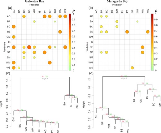
(a and b): Cross map coefficient (ρ) matrix calculated from Simplex-based CCM for Galveston Bay and Matagorda Bay, respectively. Significant causations are highlighted with circle. The size and colour of the circle indicate the strength of causation. (c and d): Cluster dendrogram of species with shared dynamic features for Galveston Bay and Matagorda Bay, respectively. The “approximately unbiased (au)” p-value and “bootstrap probability (bp)” p-value for clustering were computed by using multi-scale bootstrap resampling and normal bootstrap resampling, respectively. Species names and abbreviations are listed below: Atlantic croaker (AC), bay anchovy (BA), blue crab (BC), brown shrimp (BS), Gulf menhaden (GM), inland silverside (IS), pinfish (PF), spot (SP), striped mullet (SM), white mullet (WM), and white shrimp (WS).
Reconstructed interspecies network
Species interaction strengths estimated using multivariate S-map exhibited distinct networks of causally related species in the two bays (Figure 4) with a more complex interspecies network in Galveston Bay than Matagorda Bay. In addition, weak interactions seemed to play a dominant role in the interspecies network (Supplementary Tables S2 and S3). Pivotal species were identified including Atlantic croaker, blue crab, Gulf menhaden, pinfish, and spot in Galveston Bay, and Bay anchovy and blue crab in Matagorda Bay (Figure 4).
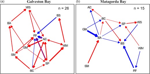
Species interaction network in (a) Galveston Bay and (b) Matagorda Bay. Red and blue colours indicate positive and negative interactions, respectively. The arrow thickness represents the interaction strength. The number of interactions is shown on the top right. Species names and abbreviations are listed below: Atlantic croaker (AC), bay anchovy (BA), blue crab (BC), brown shrimp (BS), Gulf menhaden (GM), pinfish (PF), spot (SP), striped mullet (SM), white mullet (WM), and white shrimp (WS).
Seasonality in interaction strength
Estuarine ecosystems are highly dynamic and respond to seasonal environmental changes on the timescale of days to months. We further explored the seasonal pattern of species interaction strength at a monthly time step (Figure 5). Mean species interaction strength showed strong seasonal variations in Galveston Bay with a peak in the spring months, whereas no apparent seasonality was detected on mean interaction strength in Matagorda Bay (Figure 5).
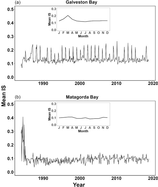
Time-varying mean species interaction strength in Galveston Bay and Matagorda Bay during the study period (1984–2018). Embedded subplots of the monthly average show the seasonality over the period. Note that interaction strengths between species were estimated by multivariable S-map.
Drivers of functional group stability
After excluding a “non-interacting” species (inland silverside) and aggregating the rest ten species into four functional groups, the drivers of functional group stability were disclosed by the CCM causality test (Figure 6). Potential drivers of function group stability were more diverse in Galveston Bay than that of Matagorda Bay (Figure 6). Temporal variation of functional groups was significantly causally affected by the ambient environmental conditions, and species diversity and interaction (Figure 6, Tables 2 and 3). Despite a relatively weak causal signal, NAO seemed to have cascading effects in Galveston Bay on local hydrology and then functional groups (Figure 6a, Table 2), while a combined influence of NAO and AMO appeared to indirectly affect the functional groups in Matagorda Bay (Figure 6b, Table 3). Notably, the stability of shrimp populations was highly susceptible to external perturbations (Figure 6).

Causal relationships between functional group stability in Galveston Bay and driving variables.
| Variables | Time lag | p-value (Kendall’s tau test) | p-value (Fisher’s Z test) | ∆ρ | Causal strength |
|---|---|---|---|---|---|
| Forage | |||||
| NAO | 5 | 0.0020 | 0.0306 | 0.13 | 0.14 |
| Discharge | 1 | 0.0008 | 0.0262 | 0.13 | 0.19 |
| Temperature | 4 | 0.0008 | <0.0001 | 0.43 | 0.66 |
| Richness | 6 | 0.0008 | 0.0001 | 0.25 | 0.31 |
| Demersal | |||||
| NAO | 4 | 0.0044 | 0.0264 | 0.13 | 0.18 |
| Salinity | 5 | 0.0008 | 0.0014 | 0.20 | 0.32 |
| Crab | 4 | 0.0044 | 0.0004 | 0.22 | 0.35 |
| Shrimp | |||||
| NAO | 5 | 0.0044 | 0.0474 | 0.11 | 0.22 |
| Discharge | 2 | 0.0020 | 0.0157 | 0.14 | 0.31 |
| Temperature | 5 | 0.0008 | <0.0001 | 0.14 | 1 |
| Diversity | 6 | 0.0008 | <0.0001 | 0.12 | 0.88 |
| Richness | 6 | 0.0020 | 0.0079 | 0.14 | 0.53 |
| IS | 0 | 0.0008 | <0.0001 | 0.34 | 0.76 |
| Demersal | 2 | 0.0008 | <0.0001 | 0.23 | 0.50 |
Note that time lag is selected based on the highest predictability. Scaled causal strengths are also given.
Causal strength is standardized for each bay.
Causal relationships between functional group stability in Matagorda Bay and driving variables.
| Variables | Time lag | p-value (Kendall’s tau test) | p-value (Fisher’s Z test) | ∆ρ | Causal strength |
|---|---|---|---|---|---|
| Demersal | |||||
| Salinity | 5 | 0.0020 | 0.0204 | 0.14 | 0.23 |
| Richness | 5 | 0.0008 | 0.0032 | 0.17 | 0.49 |
| Forage | 5 | 0.0020 | 0.0016 | 0.20 | 0.27 |
| Crab | |||||
| NAO | 1 | 0.0008 | 0.0144 | 0.15 | 0.18 |
| Shrimp | |||||
| AMO | 4 | 0.0020 | 0.0099 | 0.16 | 0.29 |
| Diversity | 1 | 0.0008 | <0.0001 | 0.12 | 1 |
| Richness | 4 | 0.0008 | 0.0216 | 0.12 | 0.56 |
| Demersal | 1 | 0.0020 | 0.0003 | 0.22 | 0.50 |
| Crab | 0 | 0.0008 | 0.0096 | 0.16 | 0.20 |
Note that time lag is selected based on the highest predictability. Scaled causal strengths are also given. Causal strength is standardized for each bay.
Ecosystem stability under climate impacts
Disparity in ecosystem stability between the two estuaries was identified (Figure 7). Galveston Bay appeared more dynamically unstable than Matagorda Bay. In addition, strong seasonality in ecosystem stability was observed in Galveston Bay, with a high state of instability in occurring in spring (Figure 7a), and in contrast, no apparent seasonality appeared in Matagorda Bay (Figure 7b).
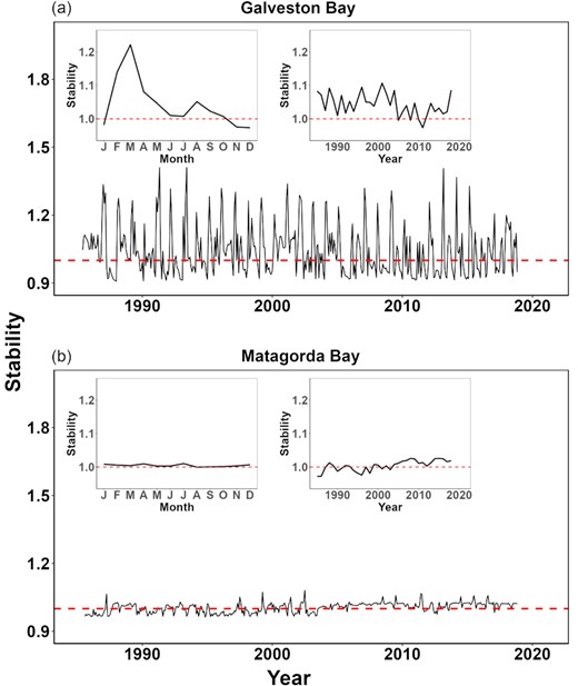
Time-varying ecosystem stability in (a) Galveston Bay and (b) Matagorda Bay. Embedded subplots show the monthly and yearly average of ecosystem stability. Red lines represent the threshold of stable/unstable dynamics. Note that ecosystem stability was estimated by using the absolute value of the real part of the eigenvalue of the time-varying interaction matrix.
In terms of causation, the dynamic stability of Galveston Bay was primarily affected by species interaction strength, followed by richness, AMO, salinity, and NAO (Figure 8a, Table 4). In addition, the lagged response of stability in Galveston Bay to NAO (6-month lag) and salinity regime (4-month lag) likely suggested potential downscaling climate effects on local hydrology and then ecosystem stability (Figure 8a, Table 4). In response, biodiversity and species interaction strength appeared to buffer the climate impacts to maintain ecosystem resilience (Figure 8a, Table 4). Despite being subjected to similar climate variability (e.g. NAO), dynamics of Matagorda Bay seemed to be stabilized by functional groups such as forage fish (Figure 8b, Table 4). CCM results are shown in Supplementary Figures S9 and S10.
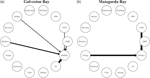
Causal linkages between ecosystem stability and other ecosystem components in (a) Galveston Bay and (b) Matagorda Bay. The arrow thickness indicates the causal strength. Note that lag effects (0–6 months) are shown in Table 4.
Causal relationships between ecosystem stability and driving variables.
| Variables | Time lag | p-value (Kendall’s tau test) | p-value (Fisher’s Z test) | ∆ρ | Causal strength |
|---|---|---|---|---|---|
| Galveston Bay | |||||
| AMO | 0 | 0.0008 | 0.0003 | 0.23 | 0.37 |
| NAO | 6 | 0.0044 | 0.0308 | 0.13 | 0.23 |
| Salinity | 4 | 0.0020 | 0.0091 | 0.16 | 0.26 |
| Richness | 2 | 0.0008 | 0.0006 | 0.20 | 0.52 |
| IS | 0 | 0.0008 | <0.0001 | 0.32 | 1 |
| MatagordaBay | |||||
| NAO | 0 | 0.0020 | 0.0171 | 0.15 | 1 |
| Forage | 1 | 0.0008 | 0.0303 | 0.13 | 0.84 |
Note that time lag is selected based on the highest predictability. Scaled causal strengths are also given. Causal strength is standardized for each bay.
Discussion
A holistic understanding of ecosystem dynamics in response to external perturbations is fundamental in ecosystem ecology and is highly needed towards the goal of EBM for marine living resources. An existing challenge is quantifying the relative impacts of external perturbations on ecosystem dynamics in view of the study scope and appropriate methodology. The present study serves as a “pseudo experiment” to distinguish latent human impacts from confounding factors by comparing dynamics of two estuarine systems with different levels of human interference using a nonparametric ecosystem modelling approach. The results show evidence of indirect human effects in combination with climate change may alter local environments, pushing an ecosystem towards an unstable state.
Biological populations exhibited distinctive dynamics between Galveston Bay (heavily developed) and Matagorda Bay (relatively undeveloped). Specifically, nonlinear dynamics were ubiquitous for populations in Galveston Bay rather than Matagorda Bay. Relevant evidence shows that the fluctuation in exploited fish stocks and their nonlinear behaviours can be amplified by fishing activities (Glaser et al., 2014), because the fisheries-induced size–age selective truncation increases the vulnerability of juvenile recruitment to stochastic environmental changes (Hsieh et al., 2006). Therefore, the nonlinear dynamics observed within the exploited populations in Galveston Bay can be largely attributed to human-induced fishing activities, since Galveston Bay receives intense fishing pressure compared to Matagorda Bay (Culbertson et al., 2004). In addition to fishing, changing environments due to pervasive human activities may exacerbate population fluctuations in Galveston Bay. Such environmental variability driving nonlinear dynamics of populations has been demonstrated by Shelton and Mangel (2011). Interestingly, unexploited fish species also exhibited nonlinear dynamics in Galveston Bay, whereas their counterparts remained stable in Matagorda Bay. Because these unexploited species often occupy lower trophic positions, the nonlinearity in their dynamics can be caused by fishing-induced volatility in predator species through a cascade of interactions (Lynam et al., 2017). For example, the nonlinearity in anchovy stocks in the Black Sea is considered as the combined result of eutrophication (bottom-up control) and fishing activities (top-down control) (Oguz et al., 2008). A lack of relevant time series, in particular lower trophic levels on zooplankton in Texas estuaries (Liu et al., 2017b, 2021), limits us to further detect the explicit cause of unstable dynamics in Galveston Bay.
Penaeid shrimp plays an important role in serving as prey items for higher trophic-level predators (Fujiwara et al., 2016), supporting the lucrative fisheries in the US GoM (Liu et al., 2017a). Of the two species in this study, the white shrimp is considered an annual species, while the brown shrimp can live up to 2 years. The short life cycle suggests that shrimp recruitment dynamics are more likely dependent upon inter-annual environmental variability. Our finding of nonlinear dynamics in white shrimp is consistent with nonlinear stock-recruitment relationship reported for white shrimp populations (Belcher and Jennings, 2004).
Despite the bio-geological similarities, dynamically equivalent clusters and the grouping patterns between Galveston Bay and Matagorda Bay were distinct, which implies that human activities may have directly and indirectly disturbed the dynamics of resident populations in the estuaries. Species sharing similar ecological attributes such as taxonomic affinity, phenology, and trophic positions normally exhibit similar dynamic features (Liu et al., 2012). To some extent, this is echoed in the present study as seen in the shared dynamics of spot, white mullet, pinfish, brown shrimp, and white shrimp. The disparity observed between Galveston Bay and Matagorda Bay in their interaction network highlighted human impacts on ecosystem reorganization, driven by decoupling intraspecific interactions (Rodewald et al., 2011; Wood et al., 2018). In general, habitat heterogeneity allows species with similar life-history strategies to partition their niches and alleviate competition (Ross, 1986). However, human-induced habitat loss may limit the within-habitat spatial and temporal separation of co-existing species, further intensifying species interactions by increasing competition and predation (Eby and Crowder, 2002; Boström-Einarsson et al., 2014). As human perturbations become more pervasive, preceding competitive hierarchies could be even reversed, leading to subordinate species with stronger adaptability dominating in degraded habitats (Tilman, 1994). Likely the result of habitat alteration or loss via coastal urbanization of the Galveston Bay species interaction network is far more complex. As such, the complex nonlinearity present in Galveston Bay may be an indicator of an unstable system that has a greater potential to shift to a degraded state.
Beyond few strong interactions, the two estuarine systems are likely maintained by more weak interactions (Supplementary Tables S2 and S3), frequently observed in natural communities (Emmerson and Yearsley, 2004). While weak interactions tend to stabilize a community by counteracting the destabilizing effects of strong interactions (McCann et al., 1998), careful attention still should be paid to strong interactions in the estuaries for future ecosystem-based considerations. For instance, strong positive feedback control of Gulf menhaden on Bay anchovy in Matagorda Bay (Supplementary Table S2) potentially implies that the collapse of Gulf menhaden can serve as an early warning of the collapse of Bay anchovy.
EBM highlights the importance of key species that include both exploited species of commercial importance and species of ecologically valuable to ecosystem functioning (Link, 2002). The present study provides an avenue for identifying pivotal species of an ecosystem assuming pivotal species as the one on which other species in an ecosystem largely depend (i.e. species interacting with at least half of other species); such that the fluctuation of pivotal species may propagate throughout the entire species network and cause ecosystem shifts. We show that despite the geographical adjacency and taxonomic affinity, species residing in the two estuaries displayed distinctive ecological roles under human interventions. For example, Atlantic croaker plays as a central role in the interaction network of Galveston Bay, while its role diminishes in Matagorda Bay. The method of identifying pivotal species shows promise for future identification of keystone species (species that are rare but crucial to the ecosystem, Power et al., 1996) for management practices.
A set of ecologically important species identified by CCM reveals the underlying causal interaction network. We note that the exact type of interaction between species may cannot be distinguished. Inter-species competition could be a major source of interaction because of the size selectivity of sampling gear. Given the sampling method, bag-seine samples largely consist of small, young-of-the-year fish and invertebrates that likely overlap on trophic positions. Due to the lack of relevant time series, further exploration about top-down and bottom-up processes is beyond the scope of the present study (but see Liu et al., 2014). One thing is clear that incorporating multiple trophic levels is conductive to better addressing the question of quantifying human impacts on interaction networks.
Species interaction strength is key to the diversity and coherence of communities (Kokkoris et al., 2002; Liu et al., 2014). Species coexistence may benefit from low mean interaction strength in natural communities, such that interaction strength decreases as richness increases (Kokkoris et al., 2002). Consistently, low species interaction strength results in high biodiversity in Galveston Bay during the summer–fall months, whereas high species interaction strength was found to emerge in spring when phytoplankton biomass peaks. Since Galveston Bay receives a considerable amount of urban and industrial nutrient-rich wastewater (Santschi, 1995), the surge of interaction strength in spring likely corroborates human interference to the eutrophic state of the bay and the following algal blooms. Subsequent juvenile recruitment may benefit from the enhanced phytoplankton and zooplankton production during the spring bloom (Liu et al., 2017b).
Large scale climate forcing on ocean conditions plays a key role in influencing biological communities (Bi et al., 2014; Liu et al., 2015; Li et al., 2022), and tends to destabilize marine food-web and ecosystem functioning (Schröter et al., 2005; Mooney et al., 2009; Chapman et al., 2020). In the present study, functional groups appeared to respond more diversely to external forcing under additional human interference (Tables 2 and 3), suggesting the role of humans in amplifying biological responses to external perturbations. Beyond that, we found evidence that climate signals such as NAO and AMO may propagate into Texas estuaries and affect functional groups by regulating local environmental conditions. The cascading climate effect on biological communities has been reported in the coastal GoM (Tolan and Fisher, 2009; Sanchez-Rubio et al., 2011). Along the Texas coast, the NAO variability has been used to explain the variations in phytoplankton (Tominack et al., 2020), benthic macrofauna (Pollack et al., 2011), and fish communities (Sanchez-Rubio and Perry, 2015; Fujiwara et al., 2019). One plausible explanation is that warm phases of NAO can result in wetter and warmer winters in coastal waters that largely influence species biology and ecology (Tolan and Fisher, 2009). Besides NAO, the AMO variability may also influence Texas estuarine dynamics. Sanchez-Rubio and Perry (2015) suggested that the NAO and AMO together regulate the wind patterns and wet regimes in the GoM, which explains the recruitment variation in Gulf menhaden (Brevoortia patronus).
Of the four functional groups, shrimp appeared to be particularly sensitive to environmental forcing. Among which, water temperature showed the strongest causal effect on shrimp populations. Studies reported that the fluctuation in the GoM shrimp populations is related to variations in water temperature (Haas et al., 2001; Li and Clarke, 2005). A recent study reported that downscaling impacts of climate-induced events in local hydrodynamics is responsible for temporal and spatial fluctuations in pelagic communities of Galveston Bay (Liu et al., 2021). As poikilothermic and short-lived crustaceans, it is reasonable that the dynamics of shrimps respond promptly to climate-driven environmental variability.
Climate threats tend to exacerbate the vulnerability of ecosystems under additional stress of human activities (Poff et al., 2002). The adverse effects of climate may lessen when ecosystems are released from human perturbations, which is seen in the present study that functional groups surpass climate-related environmental change that regulates the ecosystem dynamics of Matagorda Bay. Although Galveston Bay and Matagorda Bay are equally subject to climate controls, Galveston Bay displayed a highly unstable state, especially during the spring months. This finding suggests that human impacts can magnify the biological consequences of climate change (Harley and Rogers-Bennett, 2004). In general, estuarine pelagic communities are vulnerable to abrupt disturbance of climate-induced events such as hurricanes (Liu et al., 2021). This disruption may cause match–mismatched dynamics between predators and prey that are susceptible to climate change through bottom-up processes (Liu et al., 2017b). We notice slightly decreasing stability in Matagorda Bay over the recent decades, which implies that under climate change, coastal ecosystems may further destabilize in the future given the fact of growing populations and urbanization in coastal areas.
To some extent, findings of the present study unravel the underlying driving mechanisms of ecosystem stability of the two estuaries. Both ecosystems were found to be influenced by climate variability such as NAO, which has profound effects on the US coast (Okumura et al., 2001) including the northern GoM (Rodriguez-Vera et al., 2019). The NAO-driven changes in local environmental properties, however, may interact with one another, resulting in synergistic effects on population dynamics especially at the ecosystem level. This explains in part why few direct linkages were found between ecosystem stability and local environmental factors in the two estuaries.
A heavily utilized ecosystem tends to be vulnerable to climate change and environmental stochasticity. The resulting unstable ecosystem, however, may be alleviated by ecological processes, such as biodiversity, species interaction strength, and functional groups. Growing evidence points out the stabilizing effects of biodiversity in buffering ecosystems against environmental change (Tilman et al., 2006; Griffin et al., 2009; Campbell et al., 2011). Our findings support that biodiversity and species interaction strength are two major contributors to ecosystem stability (Ushio et al., 2018), which should be taken into ecosystem-based considerations. Specifically, the loss of biodiversity in heavily urbanized ecosystems should be given first priority on ecosystem conservation because this may impair the sustainability of ecosystem services and functions.
The relatively stable state of a less disturbed ecosystem is likely maintained by its internal functional groups, for example, forage fish tend to act as biological buffers to consolidate the stability of Matagorda Bay. Coincidently, Bay anchovy, Gulf menhaden, stripper mullet, and white mullet have been identified as essential components in the species interaction network of Matagorda Bay. As a major food source of marine predators, it is not surprising that forage fish play a crucial role in sustaining predators and ecosystem stability (Pikitch et al., 2014). Regarding EBM, careful attention should be paid to buffering species to ensure sustainable ecosystem services. We note that the effects of diversity and species interaction strength were minimal in Matagorda Bay, probably due to the relatively weak human–natural interactions. Given that intra-species self-regulation may largely contribute to the stability of interaction networks (Barabás et al., 2017), the less disturbed ecosystem may be capable of internally mitigating climate-induced environmental fluctuations such as the NAO effect found in Matagorda Bay.
The present study provides a framework for future studying on human–climate–ecosystem interactions. Indicators of human perturbation are diverse. Each indicator represents different activities. To partition the relative impacts of human influence at an ecosystem level, which indicator or a group of indicators should be included in ecosystem modelling raises an interesting issue on ecosystem modelling even without consideration of model parsimony and data availability. Although no direct measures of human impacts have been included due to data scarcity, with most confounding factors well balanced in the study design (e.g. climatology, hydrology, and ecology) and indirect reasoning by exclusion, our findings shed some light on direct and indirect effects of pervasive human activities on shifting ecosystem dynamics and stability. Later, when time series of specific human indicators become available, future study will be able to detect specific human impacts on the ecosystems, such as, fishing, pollution, coastal development, etc. for management and conservation of coastal marine ecosystems. As management of marine living resources shifts towards an ecosystem-based approach (Link, 2002), there is a need to know the extent of an ecosystem to withstand external perturbations (Gunderson, 2000; Oliver et al., 2015) and to quantify the relative importance of human activities and climate-induced environmental variability on marine living resources. While it becomes critical to account for both ecological processes (e.g. trophic interaction and biodiversity) and external forcing (e.g. environmental change and fishing), our understanding of the mechanism of the human–natural coupled dynamic system in light of climate change currently remain inadequate. Therefore, the findings of this study contribute to an improved understanding of the dynamic triangle of human–climate–ecosystem under increased climate variability.
Acknowledgement
We thank Mark Fisher for access to the Texas Parks and Wildlife Department survey data.
Conflict of interest
The authors have no conflicts of interest to declare.
Funding
This study was partially supported by the National Science Foundation under NSF grant OCE-1760463 and the Texas Sea Grant College Program’s 2022–2024 Grants-in-Aid of Graduate Research Program.
Author contributions
HL conceived of the initial idea and facilitated the study. HL and CL designed the study for the manuscript. CL applied and adapted the model with assistance from HL. CL led the writing of the manuscript with HL providing text, comments, and revisions to the manuscript.
Data availability
The datasets underlying this article were derived from sources in the public domain at
https://tpwd.texas.gov/publications/fishboat/fish/fisheries_management/mds_coastal.phtml
https://waterdata.usgs.gov/usa/nwis
https://psl.noaa.gov/data/correlation/oni.data
https://www.ncdc.noaa.gov/teleconnections/nao/
https://climatedataguide.ucar.edu/climate-data/atlantic-multi-decadal-oscillation-amo
References
Author notes
Present address: Northeast Fisheries Science Center, National Marine Fisheries Service, 166 Water Street, Woods Hole, MA 02543, USA
