


Abstract
A retrospective pattern within a stock assessment occurs when historical estimates systematically increase or decrease as data are removed and has been cited as a cause of persistent overfishing. For two case studies, Gulf of Maine cod and New England pollock, we demonstrated how closed-loop simulation can be used to evaluate the impacts of retrospective patterns with respect to management objectives. Operating models (OM) representing alternative states of nature were developed and various management procedures (MP) that account for retrospective patterns in the fitted assessment models were applied. From the cod example, downward adjustment of the catch advice based on Mohn's rho was more beneficial over model averaging (MA) to meeting biomass objectives from the cod example and avoiding stock crashes. For pollock, downward adjustment and MA were robust to meeting biomass objectives at the cost of foregone catch. The ability to discriminate OMs, using indicators generated from the simulated projections, varied by MP and time for cod, but was poorer overall for pollock. This framework could be used to identify if retrospective issues generate poor management outcomes and, in some cases, alleviate pressure to identify the single most credible state of nature.
Introduction
Stock assessments may display retrospective patterns, where estimates of stock size, and potentially stock status, appreciably and systematically change as additional years of data are added or removed from the model. The presence of a retrospective pattern is detected by re-fitting a model with successive removals of data from the most recent years (we typically refer to these truncated fits as “retrospective runs” generated by “peeling” off the data). In a well-behaved situation, one expects similar estimates in historical years that are shared among the retrospective runs. A retrospective pattern exists when estimates diverge among retrospective runs and follow a systematic pattern, e.g. biomass in a particular year decreases as more data are peeled from the model (Figure 1).
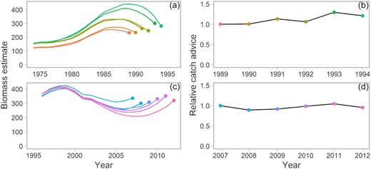
In total, two examples of the impact of retrospective patterns in biomass from assessments (a) and (c) on the corresponding resulting catch advice from a hypothetical fixed F harvest control rule (b) and (d), assuming no retrospective pattern in the target F. Points in the left column indicate the biomass estimate (and the year in which the assessment was performed) used to calculate the catch advice in the harvest control rule. From the 1994 assessment (a), the biomass trend has been decreasing and, from the 2012 assessment (c), an increasing trend is observed, yet the resulting catch advice in hindsight has remained relatively constant in both cases (b) and (d). Biomass estimates were taken from Figures 4 and 9 of Stewart and Martell (2014).
Retrospective patterns observed within a single assessment can have important implications on management advice over time. Harvest control rules (HCR) set the catch advice as a function of the estimated stock size (Deroba and Bence, 2008), and when there are severe retrospective patterns, historical catch advice from assessments fit to shorter time-series may now appear inconsistent with the more recently estimated stock trends (Figure 1). Consider a situation where successive stock assessments show that the stock trend is increasing over time but the magnitude of the estimated biomass persistently decreases with additional years of data (positive Mohn's rho; Figure 1c). If successive assessments show that the stock trend is increasing, then one would expect the catch advice from a fixed F policy to increase over time. However, the advice is driven more by the scaling issue generated by the retrospective pattern and can remain stable over time (Figure 1d). Such inconsistencies with the trend in the catch advice relative to estimated biomass trends can be explained through retrospective patterns among assessments detected in hindsight (Ralston et al., 2012; Stewart and Martell, 2014; Brooks and Legault, 2016; Punt et al., 2018).
Assessments with retrospective patterns are viewed as biased estimators of stock biomass (The term “retrospective bias” is often used to indicate that there is a retrospective trend in the model. However, it is not related to the concept of statistical bias of a model since the true state of nature is not known. To avoid confusion, we avoid using this term.). Catches that followed the prescribed advice may later be perceived to be too high in the situation with positive Mohn's rho, because later assessments will estimate past biomass to be lower than what was previously estimated (Wiedenmann and Jensen, 2018). In hindsight, the catch advice should have been lower. Thus, assessments with severe retrospective patterns are typically rejected during the peer review process (Punt et al., 2020).
Simulations have suggested that properly specified models have minor retrospective patterns, i.e. relatively low magnitude of Mohn's rho, while model misspecification tends to generate larger retrospective patterns. Depending on life history, Hurtado-Ferro et al. (2015) proposed a rule of thumb where the magnitude of Mohn's rho should not exceed 0.20–0.30 in a well-behaved assessment. Implementing time-varying dynamics in the AM, such as changes in natural mortality or survey catchability, is frequently proposed for reducing retrospective patterns (Mohn, 1999; Cadigan and Ferrell, 2005; Szuwalski et al., 2018; Legault, 2020). Other structural changes in the model, such as the choice of length- over age-based selectivity (Stewart and Martell, 2014) and choice of likelihood weighting coefficients can remove the retrospective pattern as well (Cadigan and Ferrell, 2005).
Identifying causes of the retrospective patterns is challenging because there are often multiple hypotheses that can remove the patterns (Cadigan and Ferrell, 2005; Legault, 2020). There is often insufficient data to have incorporated these hypotheses in the base model in the first place, so it is difficult to achieve scientific consensus on the causes underlying the retrospective issues. The retrospective pattern itself also does not reveal its cause nor does it reveal the direction of the bias of the model, i.e. incorporating alternative hypotheses or configurations to the model to remove the retrospective pattern can either increase or decrease biomass estimates (Legault, 2009; Deroba, 2014; ICES, 2020). The selection of one hypothesis over another often has different implications on the resulting catch advice.
With a model with positive Mohn's rho, the SSB estimate is reduced in recognition that such estimates will likely be lower in future assessments.
Nevertheless, catch advice from assessments with retrospective patterns has been cited as a contributor to the failure in achieving management objectives, such as ending overfishing and achieving optimum yield in New England (Rothschild et al., 2014). Closed-loop simulation naturally provides a coherent framework to identify how to provide the most robust management advice in light of the uncertainties with identifying the true state of nature. Alternative hypotheses on the true state of nature are incorporated into multiple operating models (OM). Algorithms for providing catch advice from fishery data are formalized in management procedures (MPs) and tested by projecting each OM forward in time with repeated applications of MPs on simulated future data (Butterworth and Punt, 1999). The robustness of MPs is defined through outcomes in the OMs relative to operationalized management objectives rather than the performance of assessments.
Closed-loop simulation also provides a framework for identifying data that can reduce the uncertainty in the set of OMs (Punt et al., 2016; Carruthers and Hordyk, 2018). Implementation of an adopted MP over time produces a response in the system dynamics, and if there are competing proposed states of nature, then there may be sufficient contrast in the dynamics such that the observed data in the future may offer support for one state of nature over the others (following the adaptive management paradigm; Walters and Hilborn, 1976).
In this study, we describe and demonstrate an approach to making progress when there are retrospective patterns in stock assessments. Rather than focusing on identifying the exact cause of the retrospective pattern, which may not be possible in the short-term, we develop multiple OMs, each of which representing an alternative state of nature and replicating the retrospective pattern in current assessments. First, closed-loop simulation identifies whether retrospective patterns are a problem by identifying which states of nature, if any, are problematic and negatively impact management performance. Second, OMs generate simulated data, which can be used to develop “indicators,” the trends and values of which could be used to identify a problematic state of nature. We apply this approach using two US groundfish stocks as case studies, Gulf of Maine cod (Gadus morhua) and New England pollock (Pollachius virens), the assessments of which, like those of many other stocks in the region, exhibit prominent retrospective patterns (Supplementary Figures C.1 and C.2). For demonstration purposes, different causes of retrospective patterns were considered between the two case studies.
Methods
In this section, we describe the steps involved in closed-loop simulation relevant for addressing retrospective patterns. Within each step, we provide the details of the application to Gulf of Maine cod and New England pollock. A summary table of abbreviations is available in Table 1.
Summary of frequently used terms, including acronyms and abbreviations. Detailed description of the models is available in the Methods section.
| Term | Description |
|---|---|
| General | |
| AM | Assessment model |
| F | Instantaneous fishing mortality |
| M | Instantaneous natural mortality |
| MA | Model averaging, a MP that averages the catch advice from two AMs |
| MP | Management procedure |
| nra | Not rho adjusted (MP) |
| OM | Operating model |
| Pmat | Proportion of mature individuals in the survey age composition, used as an OM indicator in the closed-loop simulation |
| ra | Rho adjusted (MP) |
| rho | A metric used to describe the magnitude and direction of the retrospective pattern |
| SRA | Stock Reduction Analysis, the age-structured model used as the AM in MPs and for developing OMs |
| SSB | Spawning stock biomass |
| Models | |
| M02 | Cod AM with constant M = 0.2 |
| MRAMP | Cod AM where M has increased to 0.4 |
| MC | Cod OM conditioned assuming MCs from observed values (catch is underreported) and constant M = 0.2 |
| IM | Cod OM conditioned assuming an increase in natural mortality to 0.45 |
| MCIM | Cod OM conditioned with both MCs and an increase in M |
| Base | Pollock AM with dome survey selectivity |
| FlatSel | Pollock AM with flat-topped survey selectivity |
| SS | Pollock OM with more extreme dome survey selectivity compared to Base |
| SWB | Pollock OM with dome survey selectivity; conditioning model upweighted survey likelihoods to remove retrospective pattern. |
| SWF | Pollock OM with flat-topped survey selectivity; conditioning model upweighted survey likelihoods to remove retrospective pattern |
| Performance metrics | |
| PNOF | Probability of not overfishing (F < FMSY) in the OM |
| PB50 | Probability of exceeding 50% SSBMSY in the OM |
Operating models
OMs characterize the biological and exploitation characteristics of a particular stock, as well as the observation and management implementation processes. While a single model from a stock assessment process may be the starting point for an OM, best practices typically entail incorporating a broader range of uncertainties (Punt et al., 2016). It is unlikely that a single model will be able to incorporate all uncertainties as alternative estimates of biomass, recruitment, and stock status are emergent from different proposed states of nature.
The historical dynamics of the OM were created by fitting the Stock Reduction Analysis (SRA) model using the R package MSEtool (version 2.0; Huynh et al., 2020). The SRA is an age-structured model where the fishing mortality rates (F) are calculated, such that predicted catches match observed catches. The biological parameters (natural mortality, growth, and maturity) and data (time series of catch, fishery age compositions, indices of abundance, and survey age compositions) from the assessments were used to fit the SRA (details in the Supplementary materials). For both stocks, the Northeast Fisheries Science Center (NEFSC) spring and the NEFSC fall bottom trawl surveys were used to index abundance trends, while the Massachusetts bottom trawl survey is also used for Gulf of Maine cod.
Hypothesized mechanisms causing retrospective patterns can be incorporated by modifying the data inputs, model configuration, or both. A state of nature that would explain a retrospective pattern generates a Mohn's rho close to zero in the model, a.k.a., the Rose approach (Legault, 2020). For example, if catch underreporting were the true underlying cause of the retrospective pattern, then SRA was fitted by altering the catch data accordingly. Depending on the mechanism tested, attention is also needed in the observation dynamics used to simulate future data. Using the catch example, if underreporting is believed to continue in the future, then the simulated catch observations should be reduced from the OM values.
For cod, OMs were developed with varying assumptions regarding either catch, natural mortality (M), or both. Evidence of increased natural mortality is supported by a recent estimate of M from a tagging study (NEFSC, 2013). Similar to other New England stocks, catch underreporting and increased natural mortality have been proposed to be the cause of retrospective patterns (Rossi et al., 2019; Legault, 2020; Perretti et al., 2020). The three OMs developed here had the following features:
Missing Catch (MC): assume M = 0.2 with a 44.4% catch reporting rate since 2009, i.e. the SRA was fit assuming the true catch was 225% of observed values. The misreporting starts in 2009 and will continue into the projection period.
Increased M (IM): assume a linear increase from M = 0.2 to 0.45 during 1989–2007, with M = 0.45 since 2007 and no underestimation of observed catches.
Both missing catch and increased M (MCIM): assumes a linear increase from M = 0.2 to 0.4 during 1989–2004, M = 0.4 since then, along with an 80% catch reporting rate since 2009, i.e. the SRA was fit with the true catch at 125% of observed values.
For pollock, alternative configurations regarding the survey selectivity and likelihood weights were based on observations that the groundfish surveys do not efficiently catch pollock and that larger fish can outswim the trawl gear (NEFSC, 2010). The three OMs developed here included:
Survey selectivity (SS): all selectivity at age parameters are treated identically as in the current AMs, except the value at the maximum age (9 years) is 0.05, indicating that very few old fish are caught in the survey.
Survey weighting with Base (dome) survey selectivity (SWB): the selectivity at the maximum age is 0.5, and the retrospective pattern in the SRA was reduced when the likelihood for the surveys is upweighted with a weighting coefficient of 8 (instead of 1).
Survey weighting with flat survey selectivity (SWF): the selectivity at the maximum age is 1.0, and the likelihood for the surveys is upweighted with a weighting coefficient of 10.
The fitted SRA models that generated the OMs for both case studies had Mohn's rho less than 0.15 (Supplementary Figures C.1 and C.2).
Management procedures
MPs formalize the process of conducting a stock assessment with pre-defined data inputs and model configuration, and calculating the catch advice from a HCR. Here, SRA was used as the AM and replicated the structure and output of current cod and pollock assessments, with similar retrospective patterns (Supplementary materials, Section A; Supplementary Figures C.1 and C.2). Cod and pollock each have two AMs that have been put forth for informing management (NEFSC, 2019). One cod assessment assumes constant natural mortality (M) of 0.2 (termed “M02”), while another assumes a linear increase from M = 0.2 to 0.4 during 1989–2004 and has remained high since (termed, “MRAMP”). Both exhibit positive Mohn's rho, with the magnitude smaller in MRAMP than in M02 (Supplementary Figure C.1). For pollock, the two assessments differ in assumptions on the survey selectivity (NEFSC, 2019). In the “Base” model, the survey selectivity is dome-shaped (0.5 at the maximum age), while in the alternative model (termed “FlatSel”), survey selectivity is flat-topped (1 at the maximum age). Similar to cod, both pollock models also exhibit positive Mohn's rho, with a larger retrospective pattern in FlatSel compared to Base.
For cod, five MPs were tested:
M02_nra: M02 model was used without rho adjustment to |${B_{{\rm{ref}}}}$|.
M02_ra: M02 model with rho adjustment to |${B_{{\rm{ref}}}}$|.
MRAMP_nra: MRAMP model without adjustment to |${B_{{\rm{ref}}}}$|.
MRAMP_ra: MRAMP model with rho adjustment to |${B_{{\rm{ref}}}}$|.
MA: ABC is the average of those from M02_nra and MRAMP_nra.
When the MRAMP model was used, the value of F40% was calculated with M = 0.2, following current practice (Legault and Palmer, 2015; NEFSC, 2019; Table 2).
Similarly, the five MPs evaluated for pollock were:
Base_nra: Base model was used without adjustment to |${B_{{\rm{ref}}}}$|.
Base_ra: Base model with rho adjustment to |${B_{{\rm{ref}}}}$|.
FlatSel_nra: FlatSel model without adjustment to |${B_{{\rm{ref}}}}$|.
FlatSel_ra: FlatSel with rho adjustment to |${B_{{\rm{ref}}}}$|.
MA: ABC is the average of those from Base_nra and FlatSel_nra.
For both stocks, an additional reference MP that sets the fishing mortality rate to 75% FMSY in the OM was implemented. The outcomes from the reference MP reflect perfect management of the target fishing mortality rate (defined by policy) with perfect knowledge about each individual state of nature. This MP is not possible to implement in reality and used for within-model comparisons of other MPs.
Comparison of F40%, the fishing mortality that produces a 40% spawning potential ratio, among the AMs and OMs. Description of the models are provided in the Methods and Table 1.
| Model | F40% |
|---|---|
| Cod AM | |
| M02 | 0.17 |
| MRAMP | 0.18 |
| Cod OM | |
| MC | 0.17 |
| IM | 0.18 |
| MCIM | 0.18 |
| Pollock AM | |
| Base | 0.36 |
| FlatSel | 0.37 |
| Pollock OM | |
| SS | 0.35 |
| SWB | 0.36 |
| SWF | 0.38 |
| Model | F40% |
|---|---|
| Cod AM | |
| M02 | 0.17 |
| MRAMP | 0.18 |
| Cod OM | |
| MC | 0.17 |
| IM | 0.18 |
| MCIM | 0.18 |
| Pollock AM | |
| Base | 0.36 |
| FlatSel | 0.37 |
| Pollock OM | |
| SS | 0.35 |
| SWB | 0.36 |
| SWF | 0.38 |
Closed-loop simulation and performance evaluation
For each OM, 100 simulations with stochastic recruitment deviations and observation processes were used and the projection period was 50 years. The catch advice was updated with triennial assessments and held constant between assessments. The closed-loop simulation was executed in the DLMtool R package version 5.4.3 (Carruthers and Hordyk, 2020).
Performance metrics were calculated to describe the relative benefits and trade-offs among MPs. In New England, policy dictates the need to end overfishing and potentially rebuild overfished stocks (NEFMC, 2003). Thus, performance was evaluated by calculating the probability of not overfishing (PNOF), i.e. the apical fishing mortality is less than the limit reference point of FMSY, and the probability that the spawning biomass is above the limit reference point of 50% SSBMSY (PB50) from the OMs. These probabilities were calculated over all projection years and averaged over all simulations for each MP. These legal, conservation-based performance metrics were compared against trade-offs in observed short-term catches, defined here as the mean catch during the first decade of the projection period. Long-term behaviour of the MPs was also characterized by visual comparison of SSB trajectories during the projection period and the median SSB during the last decade of the projection.
The value of MSY reference points were conditional on the OM (Table 3). The stock–recruit parameters |$\alpha $| and |$\beta $| were calculated with the unfished spawning biomass per recruit (|${\phi _0}$|) in the first year of the model along with the unfished recruitment and steepness parameters (Miller and Brooks, 2021; see Supplementary materials). A steepness value of 0.81 was used for both stocks, in the range of estimates of values for gadoids from Myers et al. (1999), and the unfished recruitment parameter was estimated in the SRA. We assumed that |$\alpha$| and |$\beta$| did not change over time because the stock would not have had sufficient time to evolve in response to a change in M (Legault and Palmer, 2015). In other words, the dynamics of the stock in the post-recruit life stage do not affect survival in the pre-recruit stage described by the stock–recruit relationship (Miller and Brooks, 2021). For the cod OMs, stock resilience to fishing decreases with higher M (and lower |${\phi _0}$|) in the projection period. Reference points associated with maximum sustainable yield (MSY), including the corresponding fishing mortality (FMSY) and spawning biomass (SSBMSY), decreased with increasing M (Table 3).
MSY reference points for the projection period in the cod and pollock OMs description of the OMs is provided in the Methods and acronyms are defined in Table 1.
| OM | FMSY | SSBMSY | MSY |
|---|---|---|---|
| Cod | |||
| MC (M = 0.20) | 0.17 | 67 829 | 9 198 |
| IM (M = 0.45) | 0.11 | 8 974 | 657 |
| MCIM (M = 0.40) | 0.15 | 14 838 | 1 436 |
| Pollock | |||
| SS | 0.41 | 125 149 | 18 017 |
| SWB | 0.42 | 96 128 | 14 139 |
| SWF | 0.44 | 79 294 | 11 909 |
| OM | FMSY | SSBMSY | MSY |
|---|---|---|---|
| Cod | |||
| MC (M = 0.20) | 0.17 | 67 829 | 9 198 |
| IM (M = 0.45) | 0.11 | 8 974 | 657 |
| MCIM (M = 0.40) | 0.15 | 14 838 | 1 436 |
| Pollock | |||
| SS | 0.41 | 125 149 | 18 017 |
| SWB | 0.42 | 96 128 | 14 139 |
| SWF | 0.44 | 79 294 | 11 909 |
OM indicators
The closed-loop feedback mechanism simulates future data when the OM is projected forward in time. Following adoption of a MP, data should be monitored to ensure that real future observations are consistent with those simulated in the closed-loop simulation (Butterworth, 2008). Alternative states of nature can exhibit differential responses among MPs, with more contrast in the system dynamics among OMs likely to produce more contrast in the future data.
We use linear discriminant analysis (LDA) as a predictive model that classifies the OM (a categorical variable) according to a set of indicators (continuous predictor variables). The term “indicator” refers to any metric that can be calculated and derived from data, e.g. mean age of age compositions sampled from the fishery or survey, and summarize the state of a system. The LDAs were fit using indicators generated from the simulated data as the training set. From the training set, the sample space (cloud of points) predicts future indicator values corresponding to various states of nature. Contrast in the sample space makes it easier to attribute a future state to an individual OM. If a MP is adopted, future data can be used to calculate the probability that the observed values are consistent with each OM. A schematic of this approach is provided in Figure 2.
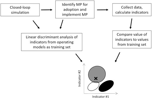
Schematic of the LDA for identifying alternative states of nature. Indicators from the OM can be used as the training set for the LDA from the projections of each MP. Following adoption and implementation of a MP, indicators can be calculated from data collected from the real system. This set of values (denoted as “X” in the lowest panel in the schematic) can be plotted against the sample space of indicators generated in the OM for the adopted MP. Indicators from each OM, representing an alternative state of nature, will have a separate sample space (denoted in white, grey, and black ovals for each of three OMs in the lowest panel). Indicators and MPs that are informative about alternative states of nature will visually generate more contrast in the sample space among OMs. The LDA calculates the probability that a future observation is consistent with each OM and characterizes whether an MP will have a high predictive power, i.e. high contrast in the indicator sample space, over time.
For both case studies, we used the mean proportion of mature fish in the survey age compositions and Mohn's rho of the AM as indicators. The nature of the misspecification relative to the OM informed the choice of indicators. For cod, persistently high mortality despite reductions in catch could be attributable to high M and inferred if there are few old, mature fish due to the truncated age structure. For pollock, dome selectivity would exclude observations of older, mature animals. For both, AM Mohn's rho can account for retrospective patterns that could persist from continued misspecification.
At each triennial assessment in the projection period, the natural logarithm of the proportion of mature fish in the simulated survey age compositions was calculated (Pmat). The mean proportions were calculated using age samples in the NEFSC spring survey from the 3 years preceding the time of calculation. Mohn's rho of the AM was calculated from 7-year peels. For each MP, the LDA classified OM with the indicators as discriminators and included an interaction effect for Year (model formula: OM ∼ Pmat × Year + rho × Year). The year covariate was included because the OMs were expected to respond differently to the catch advice from the MPs over time.
The predictive value of the indicators was evaluated in two ways. First, leave-one-out cross-validation was used to calculate the classification rate, the probability that the LDA correctly classified the OM from which the indicator originated (when individual values are omitted from the training set). The cross-validation procedure returns the posterior probability vector for assigning each out-of-sample indicator towards the three OMs (equal prior probability to assigning to each OM, i.e. one-third, was assumed). Classification was assigned to the OM with the highest posterior probability. The classification rate was calculated for each MP and assessment year. A classification rate that approaches one-third indicates little ability of the indicator to differentiate among OMs, i.e. no better than random selection.
Second, posterior probabilities were predicted across a grid of values for Pmat and rho for each MP. In this way, indicators from future data can be used to calculate the posterior probability that the observed data is consistent with each OM. From the sampling grid, a contour line was generated to predict the sampling space of the indicators that would classify with at least 50% probability to the MC OM (with missing catch) for cod and the SWF OM (with FlatSel selectivity) for pollock. With a high classification rate, a diagonal contour line over a 2D scatterplot indicates that both indicators are informative, while a horizontal or vertical line indicates one of the two indicators is informative. These OMs were chosen to separate one cause of retrospective trends from the others. For cod, the MC OM separates missing catches as the sole cause compared to higher natural mortality. For pollock, the SWF OM separates flat-topped selectivity from dome selectivity. The results of the LDA are shown for the 6th, 12th, and 18th projection year, corresponding to calendar years 2024, 2030, and 2036, respectively. These years (in the first half of the projection period) were chosen to evaluate the predictive power of the indicators as soon as possible following MP adoption. The LDA analysis, along with the cross-validation and posterior calculation procedures, were carried out with the lda and predict.lda functions from the MASS R package (Venables and Ripley, 2002).
Results
Cod
Compared to what was estimated in the benchmark assessments (M02, MRAMP), the SSB in the cod OMs was higher during the mid-2000s–mid-2010s (Figure 3a). Higher SSB is needed to support the presumed higher catches in the MC scenarios and the observed catches with higher natural mortality. Recruitment in the MC OM was higher than in the M02 model, but still lower compared to the high M (IM and MCIM) OMs and the MRAMP model. From the mid-2010s until 2018 (the last historical year), recruitment and SSB in the three OMs was lower than in either M02 and MRAMP.
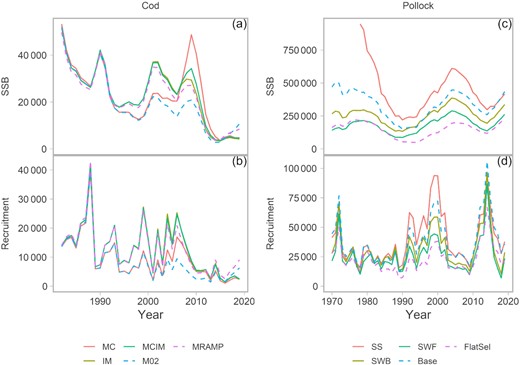
Historical SSB and recruitment estimated in the SRA for cod (a) and (b) and pollock (c) and (d). OMs and AMs are denoted in solid lines and dotted lines, respectively. Description of the models are provided in the Methods and Table 1.
In the closed-loop simulation, the reference MP (“75%FMSY”) by definition resulted in no overfishing, with PNOF > 99% and biomass above SSBMSY across all three OMs (Figure 4). By the end of the projection period, the median SSB was above SSBMSY (Figure 5p–r). The other MPs, using assessments fit to simulated data, frequently did not reduce short-term catches to those seen in the reference MP, with overfishing occurring more often than not (PNOF < 50%; Figure 4). In the MC OM, overfishing was sufficiently reduced with either the MRAMP_nra or MRAMP_ra procedures (Figure 4a), such that the stock was rebuilt above 50% SSBMSY (Figures 4a, 5g and j). Overfishing was frequently occurring with other MPs in this OM. In the high M OMs, overfishing was still occurring more often than not for all MPs (Figure 4).
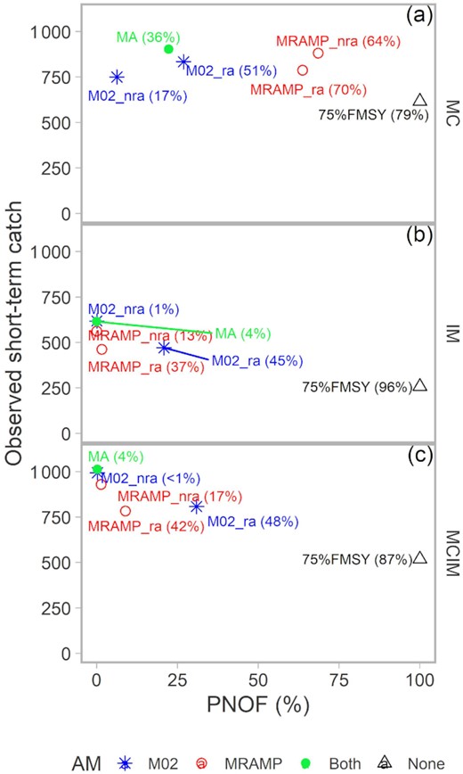
Trade-off between observed short-term catch (mean over the first decade of the projection period) and the PNOF in the pollock MPs (labels) and OMs (panels). PB50 is in parentheses. Colours and shapes indicate the AM used in the MP. Description of the MPs and OMs are in Methods and Table 1.
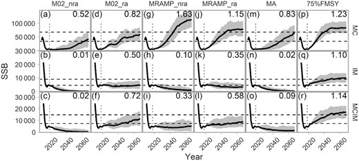
Projected SSB for the cod OMs (rows) under each MP (column). Solid lines indicate the median and the grey region the 90% CI among 100 simulations. Dashed, horizontal lines indicate 50 and 100% SSBMSY (Table 3). Dotted, vertical lines indicate the start of the projection period. Numbers in the upper right corner of each panel indicates the median SSB/SSBMSY during the last decade of the projection.
Rho adjustment substantially reduced overfishing and improved biomass outcomes (higher PNOF and higher PB50), based on comparisons of M02_nra vs. M02_ra and MRAMP_nra vs. MRAMP_ra (Figure 4). In the long run, SSB was more likely to reach and exceed 50% SSBMSY with rho adjustment than without (Figure 5; comparing columns 1 to 2 and 3 to 4). While overfishing was slightly more probable with MRAMP_ra than MRAMP_nra in the MC scenario, the former reduced F more quickly (Supplementary Figure C.3g and j). Notably, in the high M OMs, the population crashed without rho adjustment.
When no rho adjustment was made, performance was dependent on the underlying OM. Under the MC OM, MRAMP_nra outperformed M02_nra (Figure 4a), with MRAMP_nra more likely than M02_nra to rebuild the stock above 50% SSBMSY (Figure 5a and g). Higher short-term catches were achieved with MRAMP_nra over M02_nra with faster reductions in fishing mortality in the former procedure (Supplementary Figure C.3). The performance of the MA procedure was in between the other two (Figures 4a and 5m). The differences among these three MPs were trivial in the high M OMs with the SSB remaining below 50% SSBMSY (Figures 4b, c, 5b, c, h, i, n, and o). MRAMP_nra was more successful than M02_nra and MA in avoid stock crashes in one of these two OMs, i.e. MCIM.
The MC OM is frequently associated with lower Mohn's rho and higher Pmat than in the high M OMs, with the magnitude of the indicators is specific to MP (Figure 6). For example, Mohn's rho is predicted to be lower in 2030 and 2036 with MRAMP_nra and MRAMP_ra compared to other MPs, with negative values predicted for the MC OM. This is contrary to what is seen in current cod assessments (Supplementary Figures C.4 and C.5).
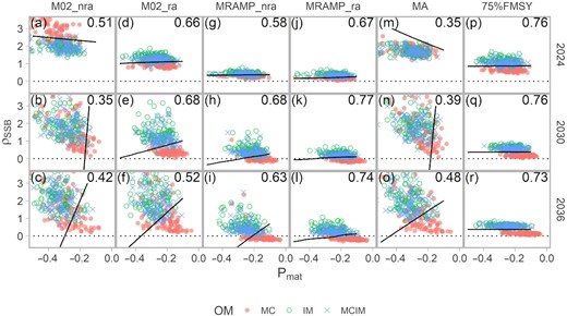
Scatter plot of indicators, SSB Mohn's rho from the AM (y-axis) and proportion mature in the survey age composition (x-axis), used in the training set of the LDA, by MP (columns), year (rows), and cod OM (colours and shapes). Proportions in the top right of each panel indicate the correct classification rate from leave-one-out cross-validation of the training set (higher predictive power with higher proportion). Black lines are the contour lines that delineate at least a 50% probability of classifying a new indicator observation to the MC OM. For the model averaging (“MA”) and 75%FMSY MPs, the Mohn's rho from the M02 AM is shown.
There is substantially more overlap in indicators between the two high M OMs, showing less ability to differentiate between these two scenarios. This pattern persists through time. The predictive skill for discriminating OMs was lowest with the M02_nra and MA MPs with low cross-validation classification rates < 50% due to high within-group variance relative to among group variance. Contour lines of poorly performing LDA models, e.g. the M02_nra MP in 2030, do not satisfactorily characterize the sample space of the indicators (Figure 6b). The prediction skill is higher with M02_ra, MRAMP_nra, and MRAMP_ra MPs with classification rates between 50 and 80%.
Pollock
Historical SSB in all three pollock OMs were higher to varying degrees compared to the FlatSel benchmark assessment, with corresponding larger recruitment to support the larger stock size (Figure 3). In the OM with extreme dome survey selectivity (SS), the SSB at the end of the historical period was similar to that in the Base assessment, despite higher values earlier in the historical period. A large initial abundance was estimated for the plus group age, which persisted through the 1970s–1980s in this OM. The historical SSB in the other two OMs (SWB and SWF) was in between that of the FlatSel and Base assessments. The SSB trends in the OMs were similar as those in the benchmark assessments.
As expected, no overfishing occurred with the 75%FMSY reference MP (Figure 7). Median SSB was fished down over time to just above SSBMSY (Figure 8p–r), with little probability of going below 50% SSBMSY (Figure 7). MPs that did not utiltize rho adjustment (Base_nra, FlatSel_nra, and MA) also had high probabilities of remaining above 50% SSBMSY, with the lowest probability of overfishing consistently with Base_nra (Figure 7). A higher probability of overfishing was associated with higher short-term catches from a windfall early in the projection period. FlatSel_nra resulted in biomass levels well above SSBMSY in all OMs at the cost of lower short-term catches (Figure 8g–i). Short-term catches and PNOF of the MA procedure were in between those of Base_nra and FlatSel_nra (Figure 7).
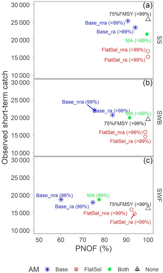
Trade-off between observed short-term catch (mean over the first decade of the projection period) and the PNOF in the pollock MPs (labels) and OMs (panels). PB50 is in parentheses. Colours and shapes indicate the AM used in the MP. Description of the MPs and OMs are in the Methods and Table 1.
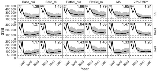
Projected SSB for the pollock OMs (rows) under each MP (column). Solid lines indicate the median and the grey region the 90% CI among 100 simulations. Dashed, horizontal lines indicate 50 and 100% SSBMSY (Table 3). Dotted, vertical lines indicate the start of the projection period. Numbers in the upper right corner of each panel indicates the median SSB/SSBMSY during the last decade of the projection.
Rho adjustment primarily reduced short-term catches when comparing Base_nra vs. Base_ra and FlatSel_nra and FlatSel_ra (Figure 7). Biomass levels were already above 50% SSBMSY without rho adjustment, so there was little scope for additional gains in PB50 with either rho adjustment or MA (Figure 8, column 1 vs. 2, and 3 vs. 4). In almost all cases, overfishing decreased with rho adjustment (Figure 7).
Compared to the cod case study, the ability to discriminate OMs was more difficult for pollock with cross-validation classification rates frequently approaching 0.33 in the LDAs (Figure 9). In the reference MP, there is significant overlap in Mohn's rho and Pmat of all three OMs (Figure 9p–r). Otherwise, higher Mohn's rho and slightly lower Pmat are seen for the OM with flat selectivity (SWF) with higher prediction skill earlier in the projection period for Base_nra and Base_ra (Figure 9a and d; classification rates above 60%). In effect, higher Mohn's rho and a larger early windfall in catches are predicted when there is misspecification in AM with regards to survey selectivity, with the Base assessment assuming dome selectivity while there was flat selectivity in the OM. Prediction skill is lower in other years and MPs (60% and lower classification rates). There is substantial overlap in indicators for OMs with dome selectivity (SS and SWB), making it is difficult to distinguish between these two. In these OMs, the FlatSel_nra and FlatSel_ra MPs can generate negative Mohn's rho, although the magnitude is relatively minor (absolute value less than 0.2; Supplementary Figure C.6).
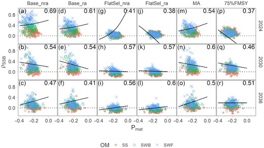
Scatter plot of indicators, SSB Mohn's rho and proportion mature in the survey age composition, used in the training set of the LDA, by MP (columns), year (rows), and pollock OM (colours and shapes). Proportions in the top right of each panel indicate the correct classification rate from leave-one-out cross-validation of the training set (higher predictive power with higher proportion). Black lines are the contour lines that delineate at least a 50% probability of classifying a new indicator observation to the SWF OM (with flat SS). For the model averaging (“MA”) and 75%FMSY MPs, the Mohn's rho from the Base AM is shown.
Discussion
Performance of management procedures
Under the presumption that there is problematic model misspecification, and facing difficulty in identifying the causal mechanisms, a closed-loop simulation framework can be used to quantify the robustness of management options that account for retrospective patterns. For cod, rho adjustment improved MP performance with respect to fishing mortality and biomass objectives. This result supports previous work highlighting the utility of rho adjustment for improving management outcomes (Deroba, 2014; Brooks and Legault, 2016; Wiedenmann and Jensen, 2019). The extent of the improvement was dependent on the true underlying state of nature, most evident when only catch underreporting caused the retrospective patterns. In this “best case” OM (OM MC), rho adjustment can reduce overfishing. In the more pessimistic OMs (high M), stock crashes are avoided but the MPs still did not sufficiently reduce short-term catch to prevent overfishing.
In a more general decision context, the results were clear regarding the ranking of MPs. To avoid the worst outcomes, rho adjustment is recommended, i.e. the M02_ra and MRAMP_ra MPs, to prevent stock crashes in the high M OMs. Between these two procedures, the trade-off in decision-making is whether to use MRAMP_ra with substantially better biological performance for the MC scenario but slightly worse biological performance for the high M scenarios. Absolute performance outcomes may exclude the adoption of the MPs evaluated here due to legal and policy requirements, but the framework demonstrates that meaningful progress towards identifying the most robust management option may still be possible despite a lack of consensus regarding the most plausible state of nature.
For pollock, model misspecification was less of a concern and the performance was more consistent among MPs. Various methods of accounting for retrospective patterns had good performance with high biomass in all three OMs. Marginal improvements were observed with further adjustments for the catch advice, but adjustments also did not degrade performance. Less yield was observed with some methods such as use of the FlatSel AM (over Base) and MA. The choice of best MP for pollock should be based on a trade-off between an acceptable risk of overfishing and potential foregone catches, which is most evident in OMs SWB and SWF (Figure 7b and c).
Rho adjustment decreases the catch advice when the sign of Mohn's rho is positive and can improve performance of HCRs. Adjustments when Mohn's rho is negative can be viewed as high risk because the catch will be adjusted upward in the advice, but closed-loop simulation can show when failure to do so is overly risk averse. We found instances of negative Mohn's rho when biomass is high, e.g. with MRAMP_ra in the cod MC scenario and FlatSel_nra in pollock. However, high or increasing biomass does not appear to be a sufficient condition for negative Mohn's rho in general (see Figure 1c). Current pollock assessments displayed positive rho despite high biomass (Figure 3; Supplementary Figure C.6). In New England, both the Gulf of Maine and Georges Bank stocks of haddock (Melanogrammus aeglefinus) have seen large increases in biomass in recent years, yet their assessments display opposite trends in the retrospective pattern (NEFSC,2019). Further exploration of the trends in the simulated data could provide insight on why retrospective patterns can substantially change over time despite no change in the forcing factors.
Model averaging is increasingly being proposed as a method for providing management advice (Anderson et al., 2017; Jardim et al., 2021), especially when there is high uncertainty about how to best model the true state of nature (Rossi et al., 2019). While averaging may be proposed in the hopes that one or several of the models adequately reflects the true state of nature, and there is reduced variance in population estimates, closed-loop simulation provides a formal setting for robustness testing. We tested the simplest case of averaging two models, both of which were misspecified to some degree relative to the OMs of both stocks. Our simulation results were mixed regarding averaging, and demonstrate that its marginal value will likely be case-specific. Averaging sometimes returned a middling performance in one performance measure or another. There was little marginal benefit for pollock assessments as high biomass could be achieved without averaging. Of course, averaging will not help in the most extreme cases, e.g. stock crashes in the high M cod OMs.
If a set of MPs do not perform satisfactorily, then more effort can be put into developing alternatives that are robust to these proposed states of nature. For example, state–space AMs could be used to detect non-stationarity in various dynamics pertaining to biological parameters (Miller et al., 2018; Miller and Hyun, 2018; Stock et al., 2021), fleet behaviour (Nielsen et al., 2021), data reliability (Van Beveren et al., 2017; Perretti et al., 2020), or some combination thereof (Cadigan, 2016). Such models may allow more flexibility in addressing the sources of the retrospective pattern, although care is needed to ensure that the models are not over-parameterized and results are not spurious (Hyun and Kim, 2022). The performance of model-based MPs can be compared to empirical, index-based MPs. Closed-loop simulation can also be used to evaluate the value of improved catch reporting (Van Beveren et al., 2020).
More conservative HCRs, e.g. with lower target fishing mortality rates or ramped HCRs that reduce the target F when the stock is declining, may also be needed (Wiedenmann and Jensen, 2019). This is an important consideration for cod, for which productivity was reduced as natural mortality increased (Table 3). Adjustments for retrospective patterns alone were not sufficient in our results and lower fishing mortality targets would be needed. All modeled pollock scenarios had similar productivity assumptions, but varied with regards to stock size. Performance outcomes for pollock were robust with respect to stock size.
The target fishing mortality rate used in the HCR here was a per-recruit quantity. Major retrospective trends are typically not apparent in selectivity estimates used to calculate the target F. In other management arenas, FMSY may be estimated from the assessment and used in the HCR. Retrospective patterns may be apparent in the FMSY estimate or the value of FMSY may be well-determined by fixing or setting informative priors on the parameters that determine FMSY, e.g. natural mortality and steepness in age-structured models and the intrinsic rate of increase in surplus production models (Mangel et al., 2013). If these parameters are estimated, then retrospective trends in FMSY may counteract or exacerbate issues with the catch advice trends shown in Figure 1.
Our results suggest that no single management option is likely to work in all situations, but the framework is sufficiently flexible to address retrospective patterns for a range of conditions that affect stock assessments. This is not to say that closed-loop simulation is without challenges. In a comprehensive analysis, a full range of suspected causes of retrospective patterns should be included in the set of OMs. For example, juvenile discard mortality of cod in lobster traps (Beonish and Chen, 2020) and changes in survey catchability have also been implicated as drivers of retrospective patterns in New England groundfish assessments (Legault, 2009; ICES, 2020). Recent poor recruitment for cod required consideration of the future productivity of the stock. While future mean recruitment generated in our simulation was similar or smaller in magnitude to values estimated in the last decade of the historical period (Supplementary Figure C.7), alternative productivity scenarios, for example, environmentally driven recruitment (Ianelli et al., 2011) or depensatory stock–recruit relationships (Liermann and Hilborn, 1997) may need to be considered in the analysis. If these OMs have disparate implications for the stock dynamics, then it may be difficult to exclude or weight these scenarios for evaluating MPs (Butterworth and Punt, 1999).
OM indicators
The LDA provides a formal method to potentially identify alternative states of nature. In the cod example, the indicators have the potential to differentiate between catch underreporting and increases in natural mortality. With exclusively catch underreporting, the tested MPs can sufficiently reduce catch to rebuild the stock to higher levels compared to today. The Pmat indicator, reflecting the recovering age structure, was higher here than in the high natural mortality scenarios. Mohn's rho tended to reduce with increasing Pmat, as well. It is more difficult to detect between a mixture of both factors (the MCIM OM) vs. natural mortality alone (OM IM), because the differences in reporting rate and M are smaller between these two.
For pollock, selectivity influences the proportion of mature fish in an age sample, but the differences in Pmat among OM scenarios were minute because the selectivity values differed primarily in the oldest and often least abundant age class. If Pmat were an informative indicator, then this approach can justify continued collection of the survey age compositions. If it is not, then alternative indicators can be proposed, including those using data not currently collected. The analysis here demonstrated that the ability to identify OMs can be dependent on time and MP. Multiple data types together can be informative, with univariate indicators developed to decrease the complexity associated with high dimensional analyses (Carruthers and Hordyk, 2018).
More broadly, indicators can only identify the OM that is most consistent with future data, but they cannot confirm the cause of the retrospective patterns. This type of analysis can inform priorities on future research given limited time and resources. For cod, low Pmat from future age samples can provide evidence of the lack of recovery in the stock resulting from high M, but verification through independent estimates of natural mortality will be highly desirable.
The indicator approach can provide an intuitive and quantitative rationale for identifying the causes underlying retrospective patterns, but there are challenges in its application. Developing an appropriate indicator is a matter of knowing where to look, which is also related to the OM scenarios that are developed in the first place. If an appropriate state of nature is not contained in the OM set, then the proposed mechanisms behind the indicators may not be valid. Continued adherence to an adopted MP is also needed. Real-life applications of MPs have frequently triggered exceptional circumstance protocols, which may necessitate re-evaluation of OM specification or ad hoc adjustments to the advice (Butterworth, 2008). In either case, the system has not behaved as characterized by the simulation. Indicators would be less helpful for identifying states of nature and decision-making if a long period of time is needed to observe the system dynamics response. Adhering to a MP that provides informative indicators is difficult to justify if the associated monitoring and/or socioeconomic costs are greater than alternatives (Smith and Walters, 2011; Walters, 2007).
Conclusion
The OM approach applied here has the benefit that it can evaluate various candidate management options under equivalent testing conditions and rank them with a focus on management performance. The impacts of potential bias in historical estimates in the AMs, relative to the OMs, on management moving forward is formally evaluated in closed-loop simulation. Several states of nature for cod were identified for which various management approaches fail to meet fishery objectives. These problematic scenarios are associated with increased natural mortality that could be identified by low Pmat and high Mohn's rho in the future. Management options for pollock, on the other hand, were more robust to the alternative states of nature related to stock size (not productivity), and the contrast in indicators was not as urgent. Overall, if there is consensus that a suitable range of hypothesized states of nature is contained within the set of OMs, then the framework demonstrated here could alleviate the pressure to identify the single most credible state of nature.
Funding
QCH acknowledges funding from the Natural Resources Defense Council.
Authors' contributions
TC acquired the funding, QCH led the analysis and writing, and all authors contributed to the writing.
Data availability statement
No new data were generated in support of this research. The R source code used in this paper is available at: https://doi.org/10.5281/zenodo.6392379
ACKNOWLEDGEMENTS
Comments from Lisa Suatoni during the initial analysis and from Tim Miller, the editor, and three reviewers on an earlier version of this manuscript were appreciated.
