


Abstract
While ecosystem-based fisheries management calls for explicit accounting for interactions between exploited populations and their environment, moving from single species to ecosystem-level assessment is a significant challenge. For many ecologically significant groups, data may be lacking, collected at inappropriate scales or be highly uncertain. In this study, we aim to reconstruct trophic interactions in the Norwegian Sea pelagic food-web during the last three decades. For this purpose, we develop a food-web assessment model constrained by existing observations and knowledge. The model is based on inverse modelling and is designed to handle input observations and knowledge that are uncertain. We analyse if the reconstructed food-web dynamics are supportive of top-down or bottom-up controls on zooplankton and small pelagic fish and of competition for resources between the three small pelagic species. Despite high uncertainties in the reconstructed dynamics, the model results highlight that interannual variations in the biomass of copepods, krill, amphipods, herring, and blue whiting can primarily be explained by changes in their consumption rather than by predation and fishing. For mackerel, variations in biomass cannot be unambiguously attributed to either consumption or predation and fishing. The model results provide no support for top-down control on planktonic prey biomass and little support for the hypothesised competition for resources between the three small pelagic species, despite partially overlapping diets. This suggests that the lack of explicit accounting for trophic interactions between the three pelagic species likely have had little impact on the robustness of past stock assessments and management in the Norwegian Sea.
Introduction
The gradual implementation of ecosystem-based fisheries management (EBFM) and associated integrated ecosystem assessments (IEAs, Levin et al., 2009) has called for models that can account for interactions between exploited populations and their physical and biological environment (Fulton 2010; Link et al., 2010; Collie et al., 2014; Guo et al., 2020). Of relevance to IEAs are models that explicitly account for trophic interactions between species or groups of species. Plagányi (2007) reviewed several such models, which include—among others—multi-species assessment models, mass balanced food-web models, size-based trophic models, and end-to-end models. The latter resolve a collection of complex processes that can include ocean circulation, biogeochemistry, trophic interactions across multiple trophic levels, population dynamics, and human pressures (including fishing).
Moving from single species to ecosystem-level modelling is a significant leap for several reasons. For many ecologically significant groups, data may be lacking, collected at inappropriate scales or highly uncertain. The rationale for including or excluding particular ecosystem components (e.g. jellyfishes, top predators, mesopelagic fauna, etc) is not always easy to clarify. It is common that some model input parameters may not be readily available, may be uncertain or may vary in time and space in ways that are not well described or understood (Levins, 1974). For example, fish diet composition is known to vary with graphical locations, seasons, years, age, and size but there is rarely enough data to describe these variations accurately. Given the high uncertainties associated with food-web models inputs—whether this concerns observations, parameters, model structure or assumptions—it is likely that different models based on the same knowledge may reconstruct different food-web dynamics.
Modelling food-webs from low to high trophic levels requires contributions from a range of experts who may have different conceptual representations of the food-web as well as different practices in collecting data and in modelling. The inclusion of participants with diverse expertise during the modelling process, from the conception of the model to the interpretation of the results, is therefore important to build trust and to allow for the appropriation of the model results.
Our point of view is that food-web models that support IEAs should (i) be inclusive of various types of expertise in all phases of the modelling process, (ii) acknowledge that input data may be lacking or may be highly uncertain, (iii) recognize that a variety of past food-web trajectories may be equally supported by available data and knowledge. One modelling framework that matches these requirements is the “Chance and necessity” modelling approach (CaN, Planque and Mullon, 2020). CaN modelling is an inverse modelling approach that explicitly accounts for uncertainties in input data/information and provides multiple possible reconstruction of food-web trajectories as outputs. CaN models are possibilistic, i.e. they explore the set of possible food-web dynamics, without assigning probability or likelihood to individual solutions (“probabilistic” models would provide these). In CaN models, food-web dynamics are controlled by the flow of biomass between ecosystem components, and these dynamics are considered possible when they are compatible with the biological and observational constraints that reflect the knowledge and uncertainties shared by multiple experts.
In this study, we use CaN modelling to quantify trophic interactions in the pelagic food-web over multiple decades, in order to support the integrated ecosystem assessment of the Norwegian Sea (ICES, 2021a). The motivation is to provide a better understanding of the energy flows within the food-web of the pelagic ecosystem and to understand the connections between these flows and the interannual changes in the biomass of commercial pelagic fish and their planktonic prey. The pelagic system in the Norwegian Sea is well studied and monitored, with regular surveys for commercial species and plankton and accurate reporting of fisheries catches (ICES, 2021a). In addition, single stock assessments for the main pelagic fish stocks provide reliable and consistent biomass estimates (ICES, 2020). There remain, however, large gaps in knowledge and observations. Most observations take place during the spring and summer months when productivity is high and when several fish species seasonally migrate into the Norwegian Sea (Skjoldal, 2004). Zooplankton patchiness and vertical migrations combined with a diversity of escaping behaviour of planktonic groups makes it difficult to obtain absolute biomass estimates for the different planktonic prey from vertical net sampling. The biomass of the mesopelagic fauna and its contribution to trophic flows is highly uncertain (Siegelman-Charbit and Planque, 2016). Prey consumption by marine mammals is imprecisely known as a result of uncertainty in abundance estimates of these groups, residence time in the Norwegian Sea, energy expenditure or diet composition (Skern-Mauritzen et al., 2022). Uncertainty in prey consumption by sea birds is to a lesser extent related to uncertainties in abundance, energy expenditure and residence time (thanks to extensive tracking and monitoring of sea birds) and mainly driven by uncertainties in diet composition (Barrett et al., 2006). Furthermore, the proportion of the annual net primary production (NPP) that is transferred to higher trophic levels is highly uncertain as this proportion depends on plankton community composition (Sigman and Hain, 2012) and trophic transfer efficiency which can be highly variable (Eddy et al., 2021). These make it challenging for experts to assess whether model results are plausible and can lead to disagreements about the role of particular species or species groups, about their abundance or contribution to the food-web, and ultimately about how these should be represented within a food-web model.
The major pelagic fish stocks in the Norwegian Sea comprise Norwegian spring spawning herring (Clupea harengus, Linnaeus, 1758), Northeast Atlantic mackerel (Scomber scombrus, Linnaeus, 1758) and blue whiting (Micromesistius poutassou, Risso, 1827) which together form the Northeast Atlantic pelagic fish complex. All three stocks perform large scale seasonal feeding migrations and overlap spatially and temporally during the feeding season (Utne et al., 2012). Several studies have investigated potentially important ecological interactions within this species complex including interspecific competition (Prokopchuk and Sentyabov, 2006; Langøy et al., 2012; Utne et al., 2012; Bachiller et al., 2016), and regulatory processes such as predation on larvae by older individuals (Skaret et al., 2015). In addition, the pelagic fish complex is reported to interact with other species such as amphipods, krill, and mesozooplankton, through both bottom-up and top-down controls (Melle et al., 2004; Olsen et al., 2007). Bottom-up control occurs when the abundance or biomass of predators is dependent on available resources from lower trophic levels, while in top-down control it is the mortality imposed by higher trophic levels that drives variations in prey biomass (Cury et al., 2003).
Due to potentially strong impact on the Norwegian Sea ecosystem, ecological interactions involving the species complex have previously been the subject of coordinated research efforts. For example, Huse et al. (2012) summarized the main findings of the INFERNO project (Effects of interactions between fish populations on ecosystem dynamics and fish recruitment in the Norwegian Sea) and concluded that “the planktivorous fish populations feeding in the Norwegian Sea have interactions that negatively affect individual growth, mediated through depletion of their common zooplankton resource.” Ibid argued for the importance of accounting for these interactions in future ecosystem-based management.
The objectives of this study are threefold. First, we aim to reconstruct an ensemble of possible trajectories of the Norwegian Sea pelagic food web during the last three decades, compatible with existing observations and knowledge. The second aim is to analyse if the model results support top-down or bottom-up controls on zooplankton (copepods, krill, and amphipods) and small pelagic fish (herring, mackerel, and blue whiting). Third, we aim to identify if there was possible competition for resources between the three small pelagic species. We stress the importance of uncertainties associated with the inputs and outputs of this modelling study and discuss the implication of the results in the context of integrated ecosystem assessment and fisheries management advice.
Material and method
The Norwegian Sea pelagic food-web
The Norwegian Sea is located northwest of Norway between 62°N and 75°N, covering an area of about 1.1 million km2. Its average depth is 1800 m (Skjoldal, 2004) and is composed of two basins deeper than 3000 m: the Lofoten Basin in the North and the Norwegian Basin in the South. The Norwegian Sea is a highly productive, seasonally mixed ecosystem with an annual reported primary production of ca. 80 to 120 gC m–2 y–2 (Rey, 2004; Skogen et al., 2007; Glen Harrison et al., 2013). The Norwegian Sea exhibits strong seasonal changes in mixed layer depths, light and nutrients conditions (Rey, 2004; Nilsen and Falck, 2006), leading to a typical spring-bloom dominated system with initial dominance by diatoms, followed by smaller flagellates as silicate becomes depleted. The spring bloom begins in May in the south-eastern part and propagates northwards and westwards (Rey, 2004). Copepods is the dominant zooplankton group in terms of abundance in the Norwegian Sea and the species Calanus finmarchicus (Gunnerus, 1770) constitutes the main part of the total zooplankton biomass (Melle et al., 2004). The larger zooplankton krill and amphipods are also abundant in this area. The Norwegian Sea is a feeding area for some of the largest exploited fish stocks in the world, such as the Norwegian spring spawning herring, blue whiting and Northeast Atlantic mackerel which feed on the aforementioned zooplankton groups (Langøy et al., 2012; Bachiller et al., 2016). While the adult fraction of the Norwegian spring spawning herring stock feeds almost entirely in the Norwegian Sea, only half of blue whiting stock is assumed to feed in the area (Dommasnes et al., 2001), and the proportion of the mackerel stock found in the Norwegian Sea is assumed to vary between 12.5% (Dommasnes et al., 2001) and more than 50% (Nøttestad et al., 2016). The deep basins and the slopes are characterised by the presence of a deep scattering layer populated by mesopelagic fauna. Commonly found species in this layer includes the armhook squid (Gonatus steenstrupi, Kristensen 1981), ribbon barracudina (Arctozenus risso, Bonaparte 1840), beaked redfish (Sebastes mentella, Travin 1951), helmet jellyfish (Periphylla periphylla Péron & Lesueur, 1810), and glacier lanternfish (Benthosema glaciale, Reinhardt 1837). The degree of trophic interaction between mesopelagic species and the epipelagic food-web is highly uncertain, though the deep scattering layer may hold a total biomass similar or greater to that in the epipelagic layer (Siegelman-Charbit and Planque, 2016). The Norwegian Sea is an important feeding area for several marine mammals (Skern-Mauritzen et al., 2022) such as fin-, minke-, sperm-, and humpback whales. Ibid study suggest that marine mammals in the Norwegian Sea consume an average of 4.6 million tonnes annually, which is significantly more than the average fisheries catch (1.45 million tonnes in the period 2006–2015). The dominant prey species of marine mammals in the area are krill (ca. 30%) followed by herring (ca. 18%), capelin and sandeel (ca. 4% each) (Skern-Mauritzen et al., 2022).
The Norwegian Sea CaN model
The food-web model for the Norwegian Sea was constructed in a collaborative manner. Two workshops were organised in December 2020 and February 2021, followed by several short meetings between February and May 2021. These were attended by members of the ICES working group on the integrated assessment of the Norwegian Sea (WGINOR, ICES, 2021a) and selected specialists for the Norwegian and Barents Sea ecosystem working at the Institute of Marine Research, Norway. These meetings were used to refine the objectives of the CaN model, to elaborate the food-web structure, to identify relevant data and to discuss the model outputs. In parallel, model input parameters were derived from literature reviews. The complete CaN model setup, including meta-information, is described in the CaN-file in Supplementary Material S1. The description of the CaN model for the Norwegian Sea food-web is provided below, following the standard ODD model description protocol (Grimm et al., 2006, 2010, 2020).
Purpose and patterns
CaN is a framework for modelling the dynamics of food-webs. The purpose of using CaN models is to reconstruct the possible trajectories of a food-web given existing knowledge and observations about its past dynamics. The objective of this study is to investigate the trophic relationships between small pelagic fish (herring, mackerel, and blue whiting) and their planktonic prey (copepods, krill, and amphipods). The primary ecological patterns are the interannual fluctuations in the biomass of these six species groups and the fluctuations in the fluxes of biomass between them and between other prey or predators. Other patterns can be derived, such as emerging trophic functional relationships, diet composition, or correlations between species change in biomass and trophic fluxes. The latter are used to address the objectives of the present study regarding trophic controls and competition for resources.
Entities, state variables and scales
In CaN, food-webs are defined by a set of components (species or tropho-species) and a set of fluxes between them (feeding interactions and fisheries). The time step of the model is annual, covering the period 1988–2020. The state variables are the biomass of the different species at each time step. In the Norwegian Sea CaN model, there are six tropho-species within the model domain (Figure 1): copepods, krill, amphipods, herring, mackerel, and blue whiting. We consider nine additional components outside the model domain which contribute to the transfer of biomass in and out of the model domain: primary producers, small mesozooplankton (< 2mm), large mesozooplankton (> 2mm), mesopelagic species, marine birds, marine mammals, predators and prey located outside the Norwegian Sea (interacting with blue whiting and mackerel) and fisheries. The model is not spatially explicit. For most species groups, the geographical extent corresponds to the Lofoten and Norwegian basins of the Norwegian Sea. For blue whiting and mackerel stocks and fisheries we consider the entire stocks/fisheries and spatial coverage is thus wider than the Norwegian Sea. Predation and feeding of these two species outside the Norwegian Sea are explicitly accounted for. The model includes 39 fluxes of biomass between the different species and fisheries.
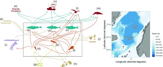
Schematic representation of the Norwegian Sea CaN model: food-web (left) and geographical location (right). (a) blue whiting, (b) mackerel, (c) herring, (d) copepods, (e) krill, (f) amphipods, (g) primary producers, (h) small zooplankton, (i) mesopelagic fauna, (j) large zooplankton, (k) resources outside the Norwegian Sea, (l) birds, (m) marine mammals, (n) fisheries, (o) predators outside the Norwegian Sea. Arrows symbolise fluxes and are coloured according to the prey group. The model domain is represented by the dashed rectangle. The biomass of trophospecies within the model domain are explicitly followed in the CaN model. For groups outside the model domain, only in/out fluxes are considered.
Process overview and scheduling
A CaN model reconstructs the dynamics of the biomass of species from the balance between ingoing fluxes (consumption or import) and outgoing fluxes (predation, export, or fisheries). The model is discrete in time and the biomasses at time t + 1 are fully determined by the biomasses at time t and the fluxes operating between t and t + 1. This is the deterministic part of the model. The fluxes between compartments are not deterministic. Instead, they are drawn randomly within a set of possible values that fulfils pre-defined constraints. This is the stochastic part of the model. The Norwegian Sea model includes 39 trophic links, which express the prey–predator interactions in the food-web, and 3 non-trophic links which represent fishing of the small pelagic fish species.
Design concepts
Basic principles
CaN models are biomass-based dynamic food-web models. The principles are similar to those outlined in other food-web models such as Ecopath (Polovina, 1984) or Ecopath with Ecosim (Christensen and Walters, 2004) with the notable differences that 1) the food-web is not assumed to be at equilibrium and 2) the trophic flows are modelled as a stochastic process, within some specified constraints (section 2.2.7) and 3) the master equation of Ecopath and CaN are slightly different (appendix 1 in Planque et al., 2014).
Emergence
The raw outputs of CaN models are time-series of all fluxes and the initial biomass of the modelled species. From these, it is possible to derive emergent properties of the food-web such as diet fractions for individual predator species, total consumption, ratios of consumption over biomass, production, throughflow, or other indices relevant to ecological network analysis (ENA, Ulanowicz, 2004; Fath et al., 2007; Guesnet et al., 2015). In this application of the CaN model, the focus is on three emergent properties: the relationship between consumption and population growth which can be indicative of bottom-up control, the relationship between predation-and-catches and population growth which can be indicative of top-down control and the relationship between consumption rates of predatory species with overlapping diets, which can be indicative of resource competition.
Stochasticity
CaN models are stochastic. The principle in CaN is to draw many random food-web trajectories within the set of possible ones. The food-web trajectories are referred to as “CaN samples.” There is no probability associated with an individual CaN sample, which represents one possible trajectory of the food-web dynamics. Thus, the CaN model is said to be possibilistic.
Observation
We derive three types of observations from CaN simulations:
Time-series of species biomass and fluxes between species/fishery
Diet composition
Correlations between biomasses and fluxes
These three types of observations can be derived from individual CaN samples. We use many CaN samples to explore the range and the distribution of these observations.
The original ODD design concepts include two additional sections entitled Adaptation, objectives, learning, prediction, sensing, and interaction and collectives. These sections are not relevant for CaN models and were not included here.
Initialization
The elements necessary to build the CaN model for the Norwegian Sea are:
The list of species and of the fluxes between them (Figure 1)
The species-specific input parameters used in the CaN master equation and to define implicit model constraints (Table 1, Supplementary Material S2)
The list of available observations, often in the form of data-series (Table 2)
The list of explicit constraints (Supplementary Material S3)
input parameter values for the Norwegian Sea CaN model. All parameters are required for species within the model domain. For prey species outside the model domain, the digestibility parameter is required. For other species outside the model domain, no parameter is required.
| Tropho-species | Satiation (σ) (kg prey.kg predator–1) | Inertia (α) (y–1) | Other losses (μ) (y–1) | Assimilation efficiency (γ) (unitless) | Digestibility (κ) (unitless) | Refuge biomass (β) (tonne.km–2) |
|---|---|---|---|---|---|---|
| Copepods | 203 | 23.6 | 12.4 | 1.0 | 0.84 | 0.01 |
| Krill | 51 | 5.98 | 5.7 | 1.0 | 0.84 | 0.01 |
| Amphipods | 25 | 3.81 | 3.1 | 1.0 | 0.84 | 0.01 |
| Herring | 12 | 0.67 | 3.4 | 0.9 | 0.90 | 0.01 |
| Blue whiting | 9.0 | 0.83 | 3.0 | 0.9 | 0.90 | 0.01 |
| Mackerel | 12 | 0.65 | 4.2 | 0.9 | 0.90 | 0.01 |
| Primary Producers | - | - | - | - | 0.65 | - |
| Small zooplankton | - | - | - | - | 0.84 | - |
| Large zooplankton | - | - | - | - | 0.90 | - |
| Mesopelagics | - | - | - | - | 0.90 | - |
| Outside resources | - | - | - | - | 0.87 | - |
| Marine Mammals | - | - | - | - | - | - |
| Birds | - | - | - | - | - | - |
| Fisheries | - | - | - | - | - | - |
| Outside predators | - | - | - | - | - | - |
list of data series used to inform and constrain the model.
| Observational series | Years span | Sources |
|---|---|---|
| Primary production | 2003–2019 | WGINOR 2021, figure 2.1 |
| Zooplankton biomass | 1995–2019 | WGINOR 2019, figure 2.4 |
| Herring biomass | 1988–2020 | WGWIDE 2020, table 4.5.1.4 |
| Blue whiting biomass | 1988–2020 | WGWIDE 2020, table 2.4.2.5 |
| Mackerel biomass | 1988–2020 | WGWIDE 2020, table 8.7.3.1 |
| Consumption/Biomass herring | 2005–2010 | Bachiller et al., 2018, figure 9 |
| Consumption/Biomass blue whiting | 2005–2010 | Bachiller et al., 2018, figure 9 |
| Consumption/Biomass mackerel | 2005–2010 | Bachiller et al., 2018, figure 9 |
| Herring diet | 2004–2016 | Unpublished results from IMR diet database |
| Blue whiting diet | 2004–2016 | Unpublished results from IMR diet database |
| Mackerel diet | 2004–2016 | Unpublished results from IMR diet database |
| Herring catches | 1988–2019 | WGWIDE 2020, table 4.4.1.1 |
| Blue whiting catches | 1988–2019 | WGWIDE 2020, table 2.3.1.1 |
| Mackerel catches | 1988–2019 | WGWIDE 2020, table 8.4.1.1 |
| Mackerel proportion in the Norwegian sea | 2007–2014 | Nøttestad et al., 2016 |
The biomass of species at the start of the modelling time-period (year 1988) constitutes the initial conditions. These do not need to be specified in the initialisation phase as they are sampled during CaN modelling.
Input data
Many data time-series for the Norwegian Sea ecosystem are compiled and reported annually by WGINOR (ICES, 2021a). In addition to these series which mostly originate from dedicated monitoring programs, there are single observations, i.e. for one or few years only. Some input data are directly derived from field measurements, like survey indices of zooplankton biomass (ICES, 2021b). Others can result from complex modelling operations, such as fish stock biomass derived from fish stock assessment models (ICES, 2020) or net primary production derived from satellite‐based primary production models (Arrigo and van Dijken, 2011). Diet data for herring, mackerel and blue whiting have been collected through stomach sampling programs (Langøy et al., 2012) starting in 2004 and total consumption estimates for small pelagic fish species are taken from bioenergetic model results (Bachiller et al., 2018). The complete list of input data series and single observations used in this study is provided in Table 2.
Model constraints
Constraints are specific to CaN models (and therefore not listed in the items of the ODD protocols). In CaN models, constraints express our knowledge about the system, and how we distinguish possible from impossible dynamics. CaN model outputs are stochastic solutions within a set of predefined constraints. All CaN models contain implicit/compulsory constraints which reflect that: biomasses are always positive, fluxes are always positive, the growth and mortality rates of a tropho-species is bounded (inertia constraint) and feeding by unit time/biomass is also bounded (satiation constraint). Additional explicit constraints can be specified to reflect additional knowledge about the food-web, such as information on the production, biomass, or consumption of different trophospecies. Explicit constraints are written in the form of symbolic expressions (equalities or inequalities) that relate model components, fluxes, and observations. CaN model deals with uncertainties through the use of constraints. For example, if the biomass of an animal group is not monitored but has been inferred to be between a minimum and a maximum bound, the food-web dynamics can be constrained to maintain the species biomass within these bounds. Similarly, if diet data is available for some groups for some years, these can be used to constrain the possible food-web trajectories within these dietary limits. The method for constructing different types of constraints is further developed in Drouineau et al. (2021).
The CaN model for the Norwegian Sea includes several types of constraints. Constraints on biomasses indirectly restrict trophic and non-trophic fluxes. Constraints on fish catches directly affect fluxes from pelagic fish to fisheries. Constraints on satiation directly limit incoming fluxes for the six species within the model domain. Constraints on NPP directly affect fluxes from primary producers to copepods and krill and indirectly affect fluxes from small zooplankton to copepods and krill. Constraints associated with diet or total consumption estimates affect the fluxes from zooplankton and mesopelagic fauna towards small pelagic fish. The range of possible biomass for the six main species is additionally constrained by inertia, refuge biomass and compliance with biomass observations. While some constraints apply for the entire model period (1988–2020) others only apply for selected years when appropriate data were available. In total 120 constraints were used in this study. The list of constraints used in this model, their period of application as well as their sources can be found in Supplementary Material S3.
Submodels
Sampling of CaN trajectories is achieved using a Gibbs polytope sampling algorithm which is efficient for problems of high dimensionality (Aditi and Vempala, 2020; Drouineau et al., 2021). A total of 100 000 food-web trajectories were sampled and only one for every 100 samples were retained (a procedure known as thinning, designed to avoid dependence between MCMC samples). The resulting 1000 trajectories were analysed to explore past food-web trajectories and trophic-controls.
Summary
The Norwegian Sea CaN model is a food-web model defined by (i) six main trophospecies and nine additional components, (ii) 39 fluxes, (iii) a master equation that relate biomass to fluxes, (iv) 6 input parameters for each species, (v) 4 species-specific implicit constraints, (vi) 120 explicit constraints, and (vii) 15 sets of observational data.
The steps for the implementation of CaN models include (i) model design (defining the components and the fluxes), (ii) entry of input parameters, (iii) provision of observational data, (iv) definition of explicit constraints, (v) construction of the system of in/equalities that defines possible trajectories, (vi) sampling possible trajectories and (vii) graphical representation and analysis of the model results.
The model was built using the R library RCaN and the Java graphical user interface RCaNconstructor (Drouineau et al., 2021, available from https://github.com/inrae/RCaN), which integrate all these steps into an interactive platform that can be used in a collaborative manner.
Analysis of CaN model outputs
The primary outputs of CaN models consist of time-trajectories of the biomass and fluxes. These provide a first level assessment of the past dynamics of the food-web. This assessment consists of a multitude of possible trajectories which express the uncertainties about past biomass and fluxes. These uncertainties reflect the degree of precision in the input knowledge and data. From these trajectories, it is possible to derive additional patterns that are relevant for the investigation of the food web dynamics. These patterns include for example the representation of diet fractions i.e. the proportion of different prey in the diet of individual predator species.
The present study investigates trophic controls, either by predation pressure (top-down) or by resource availability (bottom-up). For this purpose, we quantify the relationship between individual species growth and the relative predation pressure (the fluxes going out) and food consumption (the fluxes coming in). Species growth is defined as the ratio of species biomass between two time-steps |${B_{i,\,\,t + 1}}/{B_{i,\,\,t}}$|. Relative predation pressure is defined by the sum of outgoing fluxes relative to the species biomass |$\mathop \sum \nolimits_j {F_{ij}}/{B_{i,\,\,t}}$|, while relative consumption is defined by the sum of ingoing fluxes relative to the species biomass |$\mathop \sum \nolimits_j {F_{ji}}/{B_{i,\,\,t}}$|. We computed Pearson correlation coefficient between species growth and consumption to assess the support for bottom-up control. We also computed the Pearson correlation coefficient between species growth and predation to assess the support for top-down control.
We investigated the potential for competition by correlating the trajectories of relative consumption between pelagic fish species. A negative correlation is indicative of resource competition i.e. when one species consumes more the other consumes less and vice-versa. The competition was investigated by comparing consumption of all planktonic prey (total consumption) and by comparing consumption of individual prey groups (prey-specific consumption).
For the trophic control and competition analyses, we computed the Pearson correlation coefficients for each CaN trajectory. We then use boxplots to visualise the distribution of the correlation coefficients based on the full set of trajectories.
Model evaluation
The evaluation of the model was performed based on the match between observed and simulated ecological patterns. These patterns primarily include time-series of biomass and fluxes, and diet patterns. The sampling performance of the model was also diagnosed by inspecting that the MCMC sampling chains were mixing properly and were not autocorrelated. A sensitivity analysis was conducted by varying the main input parameters and assumptions. A model evaluation report was finally prepared, following the OPE protocol (Objectives, Patterns and Evaluation, Planque et al.,in press).
Results
The primary output of the CaN model is a set of possible food-web trajectories. Each trajectory is composed of six biomass time-series and 39 flux time-series that are compatible with each other and with every model constraint.
Biomass trajectories
The envelopes of the biomass trajectories of the six species reflect the uncertainty around the input observational data. The biomass time series of the pelagic fish are constrained by precise observational time-series (i.e. stock assessment outputs) and have therefore relatively high precision (Figure 2, bottom row). For the zooplankton groups (Figure 2 upper row), individual trajectories are more uncertain and display high year-to-year variations within broad envelopes. Individual time-series tend to reach extreme high or low biomass (i.e. close to the limit of the envelope) in at least one year of the sampling period 1988–2020.
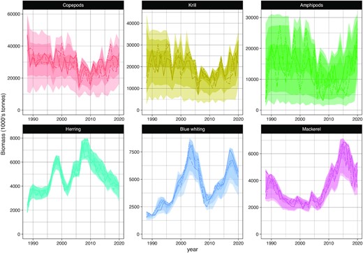
Reconstructed time-series of biomass for the six species within the model domain: copepods, krill, amphipods, herring, blue whiting, and mackerel. Each panel shows the envelopes containing 100% (light), 95% (medium) and 50% (dark) of the 1000 sampled trajectories. Three individual trajectories are provided for illustration in plain, dashed and dash-dotted lines.
Fluxes trajectories
The envelopes of the flux time-series highlight how certain or uncertain the reconstructions of historical fluxes may be, given currently available data and knowledge (Figure 3). For the consumption of primary producers by copepods, CaN reconstructions range between 300 and 800 Mt.year–1. No clear temporal trend can be detected while there is high variability between years and between CaN trajectories. Compared to the consumption of primary producers by copepods, the consumption of copepods by herring is provided with slightly less uncertainty, and in particular for the period 2004–2016 when estimates of consumption are available from survey-based stomach contents analysis. Note the higher uncertainties in years 2008 and 2011 when these estimates were not available. The reconstructions of fluxes from the herring population to the fishery are heavily constrained by the catch data, which are known with high precision. As was the case for the biomass time-series, the flux time-series display high year-to-year variations and reach extreme high or low fluxes (i.e. close to the limit of the envelope) in at least one year of the period 1988–2020. The complete set of reconstructed fluxes is provided in Supplementary Material S4 (Figure S4.1).

Reconstructed time-series of three selected fluxes: primary producers to copepods (left), copepods to herring (middle) and herring to fisheries (right). Each panel shows the envelopes containing 100% (light), 95% (medium) and 50% (dark) of the 1000 sampled trajectories. Three individual trajectories are provided for illustration in plain, dashed and dash-dotted lines.
Diets
It is possible to derive the proportion of prey in the diet of copepods, krill, amphipods, herring, blue whiting, and mackerel (Figure 4) from the CaN reconstructions. These diets reflect the information provided in the constraints (e.g. constraint 28 which specifies that the proportion of small zooplankton in the diet of copepods cannot exceed 20%, or constraints 41 and 42 which relate the consumption of copepods by herring in the model to the consumption reported in field observations). These diets also reflect the dynamic balance between resource requirements and prey availability which is expressed in the CaN master equation. From these results, the diets of herring, blue whiting and mackerel appear to be diversified and overlap with each other (Figure 4-top), though blue whiting and mackerel consume prey outside the Norwegian Sea. When averaged over many trajectories, the diets display little interannual variability, except for years when diet observations were readily available, as exemplified for herring (Figure 4-middle). Estimates from individual model trajectories highlight within-year uncertainties in the proportion of individual prey in the diet (Figure 4-bottom).
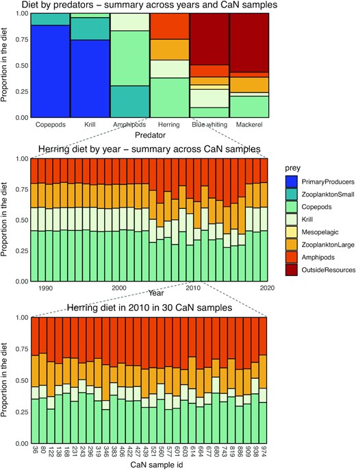
Reconstruction of diets. Average diet for each of the six modelled species (top), annual diet for herring in individual years averaged over all CaN samples (middle), and herring diet in one year (2010) for 30 selected CaN samples. The height of coloured bars indicate the proportion in the diet for each prey consumed.
Trophic controls on population growth
For herring, there is a clear positive relationship between total consumption and population growth across all trajectories (Figure 5-left), despite uncertainties in the consumption of individual prey (Figure 4 and S4.1). This is in line with a possible bottom-up control. On the other hand, there is no clear relationship between herring population growth and predation-and-catches (Figure 5-right), which suggests that top-down control is not operative. The distribution of the correlations—between population growth and consumption/predation—calculated at the individual trajectory level (Figure 6, bottom-left) confirms the support for apparent bottom-up control and lack of support for top-down control. A similar pattern is observed for copepods, krill, and amphipods (Figure 6, top row). For blue whiting the positive correlation between consumption and population growth also exists but it is slightly weaker (Figure 6, bottom-centre). In addition, the correlation between growth and predation-and-catches is negative. This pattern is even stronger in the case of mackerel (Figure 6, bottom-right). These results indicate that the model outputs can potentially support both top-down and bottom-up hypotheses for mackerel. A detailed examination of individual model outputs reveals that reconstructions that are most supportive of bottom-up control are little supportive of top-down control and vice-versa (Figure S4.2).
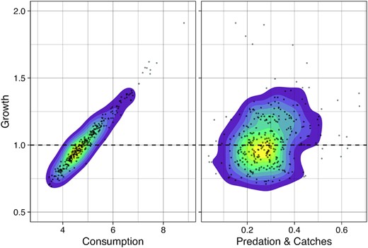
The relationship between population growth of herring and consumption (left) and between population growth and predation-and-catches (right). Each dot represents the estimated growth and feeding/predation for a given year, in a given CaN sample. The coloured density contours help to visualise the shape of the scatterplot. Growth is expressed as the ratio of biomass at time t + 1 over biomass at time t. Consumption, predation and catches are in kg consumed/predated during the time interval t to t + 1 per kg of biomass at time t.
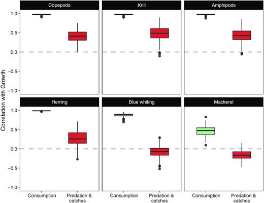
Distributions (boxplots) of the correlation coefficients between population growth and consumption (green) or predation-and-catches (red).
Competition between small pelagic fish
The correlations between prey consumption by herring, mackerel and blue whiting are generally close to zero, which is indicative of absent or weak competition for resources between the three species (Figure 7). However, these correlations vary between pairs of predators and for the different prey consumed. The negative correlation between blue whiting and herring consumption of copepods (Figure 7 top-left) suggests that the two fish species could compete for this resource. Similarly, the negative correlation between mackerel and blue whiting consumption of large zooplankton (Figure 7 top-right) is indicative of possible competition for this resource. Opposingly, the correlations for amphipods (Figure 7 middle-right) are mostly positive, which indicates that the three small pelagic fish are not competing for amphipods but rather feed opportunistically on this resource when it becomes available. The negative correlation between the total consumption (i.e. all prey combined, Figure 7 bottom) of herring and mackerel suggests a possible but limited competition between the two species, when all prey are jointly considered.
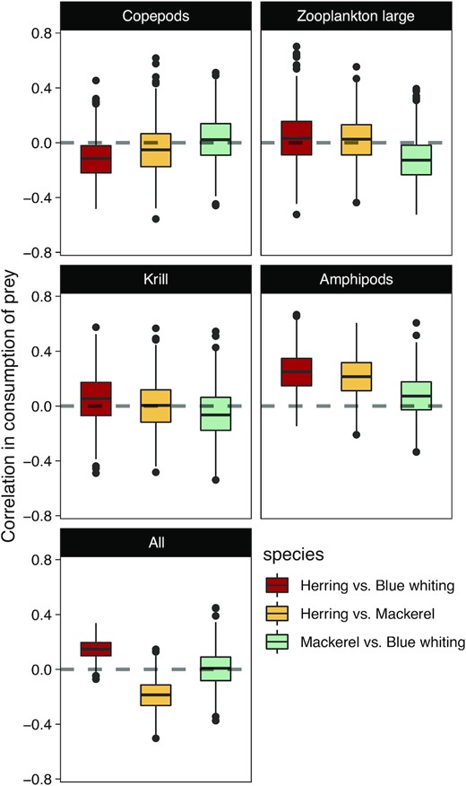
Distributions (boxplots) of the correlation coefficients between herring, mackerel, and blue whiting consumptions in the Norwegian Sea for different prey species. Positive correlations are indicative of similar interannual variations in consumption between predators. Negative correlations are indicative of competition.
Discussion
Trophic interactions between small pelagic fish and their prey
Using CaN modelling we have reconstructed multiple food-web trajectories for the Norwegian Sea. The variations between these trajectories reflect uncertainties in the input knowledge and data that support the model. From these trajectories we have reconstructed the diets of herring, mackerel, and blue whiting and of their planktonic prey: copepods, krill, and amphipods. We have estimated correlations between population growth, prey consumption and predation and catch. Our results show that for all species there is a positive correlation between population growth and consumption of prey, supportive of a possible bottom-up control. This support is strongest for herring and weakest for blue whiting and mackerel. For the latter two species, our results indicate that population growth could possibly have been limited by losses, either through predation or fisheries. Some CaN reconstructions support bottom-up control for blue whiting, independent of a possible top-down mechanism (Figure S4.2). For mackerel, trajectories with positive growth-consumption relationships often display weak or absent growth-predation relationships and vice-versa (Figure S4.2). This indicates that given the available inputs, the models outputs can be either supportive of a moderate bottom-up control, a moderate top-down control or a mixture of both trophic controls.
Our results also suggest limited support for interspecific competition between the small pelagic species at the population scale. The dynamics of herring and mackerel show slight negative covariations in consumption when all prey species are considered jointly. On the other hand, blue whiting and mackerel consumptions vary independently, and blue whiting and herring consumptions are positively related (Figure 7, bottom-right). Resource limitations may have occurred in cases when herring and blue whiting were feeding predominantly on copepods (Figure 7, top-left). The model results show no evidence of competition for krill, while the positive correlations on amphipods consumption suggest that this resource is opportunistically preyed upon by the three small pelagic fish.
These results are in contrast with previous studies that have argued for strong top-down controls by planktivorous fish on zooplankton (Skjoldal, 2004; Huse et al., 2012). Large stocks of herring and concomitant increases in blue whiting have been correlated with low copepod biomasses the following year (Olsen et al., 2007). Similarly, long term trends seem to indicate a decreased zooplankton biomass matched by an increase in planktivorous fish biomass (Huse et al., 2012). It has also been suggested that small pelagic fish may compete for limiting resources at local scales and that this can affect somatic growth (Huse et al., 2012; Olafsdottir et al., 2016).
A recent modelling study, assessing the impact of sampling design on zooplankton biomass estimates, suggests that the above zooplankton trends are highly uncertain, mainly as a result of zooplankton patchy distribution (Hjøllo et al., 2021). While previous works have focused on the copepod species Calanus finmarchicus, the dominant mesozooplankton species in the Norwegian Sea (Melle et al., 2004), the CaN model presented here includes multiple prey groups. This provides more flexibility to account for possible changes in diet or in trophic controls that are known to vary spatially and seasonally (Olsen et al., 2007; Varpe and Fiksen, 2010).
Interspecific competition depends on the degree of spatiotemporal overlap between predator species. Even when species do co-occur, intra- and interspecific competition implies resource limitation. Bachiller et al. (2016) reported dietary overlap between herring and mackerel to be larger when the fish co-occurred indicating that the species were predating on the same zooplankton patches. In addition, they argued that the lack of prey switching indicated limited interspecific competition. In our study, we found possible but limited competition between mackerel and herring which is in accordance with Utne et al. (2012) who, based on a modelling study, reported only a minor increase in annual consumption when species were simulated individually (i.e. with no interspecific competition). We found indication of possible competition between blue whiting and herring feeding on copepods, but no further indication of competition between blue whiting and the two other pelagic species when all prey species are considered jointly.
Model uncertainties, sensitivities and limitations
Uncertainties in the outputs of the CaN model presented here are generally high, at least in comparison with other commonly used food-web models for the same region (Skaret and Pitcher, 2016; Bentley et al., 2017; Pedersen et al., 2021). This may appear, at first sight, as a limitation of the CaN modelling approach. Rather, we contend that these high uncertainties provide an accurate representation of uncertainties in input data and knowledge. Constructing a CaN model compatible with the entire set of available input information is an iterative process during which “precise but wrong” models are gradually eliminated by relaxing model constraints or decreasing certainty in some of the input observations. This process is a way to identify where information might be lacking, biased, not easily scalable to the entire Norwegian Sea or simply uncertain. One key feature of the CaN models emerging from this process is that the outputs—i.e. all individual food-web trajectory sampled with CaN—are always compatible with the entire set of input data and knowledge. This is often not the case for EwE models for which at least part of the past observations lie outside the confidence bounds of the model outputs (see for example Figure 5 in Bentley et al., 2017; and Figure 2 in Pedersen et al., 2021).
It is possible to draw robust conclusions on trophic controls and competition for the three pelagic fish stocks and their prey in the Norwegian Sea, despite the large uncertainties in individual biomass and trophic flux estimates. This is because all food-web components are linked to each other and to the input observations, thereby constraining the range of possible trophic interactions.
As with any model, the results obtained with the CaN model and the conclusions drawn from them depend on model assumptions and on the values of input parameters. Presently, it's not yet possible to handle uncertainty in model input parameters in the RCaN library used to operate CaN modelling. The sensitivity of the model to uncertain parameter values can nonetheless be assessed through standard sensitivity analyses (EPA, 2009). We explored the sensitivity of our main conclusions to a range of parameter values and assumptions, including primary production, fishing intensity, other losses, inertia, satiation, the geographical distribution of blue whiting and mackerel, and predation pressure by marine mammals (Supplementary material S5). Decrease in primary production leads to reduction in the biomass of copepods, krill and amphipods but does not alter the conclusions regarding trophic controls. Beyond 75% reduction in primary production, it is not possible to reconstruct food-web dynamics that are compatible with the input data. Assuming higher (>25%) fisheries catches than reported leads to slightly higher positive correlations between mackerel and blue whiting consumptions. Changes in other losses tend to reinforce or dampen the perception of some trophic controls. For example, support for top-down control of blue whiting decreases when other losses for krill changes (positively or negatively) and when other losses for blue whiting declines. Reduced other losses for herring leads to greater support for synchronous opportunistic feeding by herring, blue whiting and mackerel on amphipods. Model results are little sensitive to variations in inertia except in the case of krill, where higher inertia leads to reduced evidence for top-down control on blue whiting. Variations in the satiation parameter for copepods, krill, amphipods and blue whiting alter the support for top-down control on blue whiting. Decrease and increase in the satiation parameter for mackerel respectively strengthens or weakens the support for top-down control for this species. Increase and decrease of the proportion of blue whiting in the Norwegian Sea leads to respectively weaker and stronger support for top-down control on blue whiting. Changes in the proportion of mackerel in the Norwegian Sea have consequences on the support for top-down control on mackerel, support for competition between mackerel and herring (on all resources combined), and the support for top-down control on blue whiting. Increased predation pressure by marine mammals leads to a greater support for possible top-down control on blue whiting and mackerel, and a lesser support for bottom-up control for these two species. In summary, the model results can be altered when using extreme values of primary production, other losses, spatial distribution, and top predator pressure. Future modelling attempts would gain from more precise estimates of these input parameters and constraints. Trophic controls on blue whiting were most often altered and those on mackerel were sensitive to a lesser extent. Overall, the main conclusions derived from the CaN model outputs can be slightly reinforced or dampen, but are generally robust to uncertainties in model parameters and inputs. An extensive description of the model evaluation is provided in Supplementary Material S6.
The CaN model presented here is not spatially or seasonally explicitly. This implies that the key processes relating predators and prey dynamics have been summarised over the whole Norwegian Sea and on an annual basis. This does not permit a detailed investigation of the processes occurring at smaller/shorter spatial and temporal scales which may have driven observed changes in biomass and diets. The apparent lack of interspecific competition could be explained by differences in phenology with different timing of the main/peak feeding season (Langøy et al., 2012) and/or behavioural differences in their daily movement patterns (Debes et al., 2012). Furthermore, changes in migration behaviour may also have been a major factor affecting food availability and the potential for competition between pelagic fish. The standing biomass, production, and spatiotemporal dynamics of zooplankton during the feeding season may affect the pelagic fish complex. Separate areas and water masses in the Nordic seas differ in the relative abundance of zooplankton during the feeding season due to differences in, among others, growth rate, species composition and seasonal vertical migration (Dalpadado et al., 1998; Broms et al., 2009; in, prep.; Bagøien et al., 2012). Generally, the seasonal zooplankton development in the Norwegian Sea and adjacent areas is progressively delayed from southeast to northwest and from coastal- to Atlantic and further to Arctic waters (Broms and Melle, 2007; Bagøien et al., 2012). The feeding migration pattern of herring have been suggested to follow spatial gradients in prey availability (Broms et al., 2012) and the geographical expansion of mackerel since the mid-2000s have partly been explained by food limitation (Olafsdottir et al., 2019).
Contribution to integrated assessment and management
Ecological models are important tools to perform marine integrated ecosystem assessments. The present modelling study was stimulated from discussions within the IEA group for the Norwegian sea (WGINOR, ICES, 2021a). Ecological observations on their own could not clarify matters concerning competition between the small pelagic fish species and the role of their main zooplankton prey. Food-web modelling represents a suitable approach to integrate existing information, but this is further complicated by uncertainties and variability in many ecological parameters, and the lack of precise population estimates of biomasses and trophic fluxes. Building and tuning ecosystem models often requires extensive time and effort (Plagányi, 2007), and the resulting models may be perceived as “black boxes” for non-modelers. The Norwegian Sea CaN model is relatively simple and presented in a transparent manner, which provides an opportunity for participatory modelling. This, in turn, promotes better communication and a sense of ownership of the model and its results by a wider community. Adding new observations and modifying model constraints is straightforward in CaN models. This flexibility supports joint explorations of the model results under varying assumptions and input data, which favours trust building between modelers, experimental and observational scientists. Because the precision of the model outputs is directly related to the precision of the input information, CaN modelling is helpful to identify critical inputs and where these might be lacking or be of insufficient quality.
A key task of the IEA group in the Norwegian Sea is to consider if single-species assessments could be improved by adding multispecies interactions, and in particular trophic ones. In a way similar to single-species assessment, which are used to reconstruct populations’ dynamics, CaN model can reconstruct past dynamics of the food web, and can provide insights into past and present multispecies interactions that can inform management. The present CaN model results do not support resource competition as a main driver for the dynamics of individual small pelagic fish populations, which points to a likely limited impact of including competition for the management of herring, mackerel and blue whiting. On the other hand, the population growth of the three species is tightly coupled to their prey consumption which could point towards a possible use of zooplankton monitoring data to directly inform management. This can however be challenging. In a recent modelling study, Kaplan et al. (2020) added the level of mesozooplankton as a control mechanism in the harvest control rule for mackerel but this resulted in higher variability, both in the catches and in the biomass of the mackerel. The potential large uncertainties associated with zooplankton biomass estimates (Hjøllo et al., 2021) add a further challenge to the prospect of incorporating zooplankton into management. In addition, the CaN results do not show any evidence for a relation between zooplankton consumption by small pelagic fish and available zooplankton biomass. So, while fluctuations in pelagic fish population growth have been tightly coupled to consumption during the last three decades, this doesn't entail that food resources have necessarily been limiting.
Though ecosystem models have been available for several decades (e.g. Ecopath with Ecosim, Polovina, 1984; Walters et al., 1997; Christensen and Walters, 2004; Heymans et al., 2016), they remain underused in management (Hyder et al., 2015; Skern‐Mauritzen et al., 2016; Schuwirth et al., 2019). Some major challenges are the large uncertainties, the lack of transparency that emerge from their complexity, and the difficulty to communicate complex models to stakeholders (Plagányi and Butterworth, 2004; Lehuta et al., 2016; Grüss et al., 2017; Schuwirth et al., 2019; Steenbeek et al., 2021). The CaN framework presents the advantage of explicitly including data uncertainties, of avoiding explicit representation of complex processes that are difficult to observe or parameterise, and of presenting assumptions, parameters, data, and outputs in a transparent manner (Planque and Mullon, 2020). These elements support efficient communication of the modelling approach, assumptions and outputs to peer scientists and stakeholders.
The primary objective of the model presented here was to quantify the dynamics of past trophic interactions in the Norwegian Sea food web from available observations. This is comparable to single stock assessment models that aim at reconstructing past populations dynamics from observations, but extended to a simplified food-web. Like single stock assessment models, the CaN model leaves aside many of the detailed processes that could underpin the reconstructed dynamics (for example migrations & spatial distributions of predators and prey). These need to be addressed elsewhere and CaN would benefit from being used in conjunction with other modelling approaches, such as single stock assessment, spatial distribution, or bioenergetic models, to inform management (Lewis et al., 2021).
Conclusion
Reconstructing the past dynamics of marine food-webs is a challenge because many species and trophic fluxes are poorly sampled and because model inputs are often highly uncertain. Using CaN modelling we have reconstructed an ensemble of possible past dynamics for the Norwegian Sea pelagic food-web, with focus on the three main small pelagic fish species and their planktonic prey. Our reconstructions are fully compatible with existing observations and knowledge. We show that despite large uncertainties in reconstructed food-web dynamics, it is possible to draw conclusions on the trophic interactions in this system. Population growth of copepods, krill, amphipods and herring are tightly coupled to consumption. For blue whiting, the relationship between growth and consumption is positive but weaker. In the case of mackerel, it is not possible to firmly establish whether population growth is predominantly related to consumption or to predation-and-catches. We found no evidence for top-down control on planktonic prey and little evidence for resource competition between the three small pelagic species. This suggests that the lack of explicit accounting for trophic interactions between the three pelagic species likely have had little impact on the robustness of past stock assessments and management in the Norwegian Sea.
Data availability statement
The set of input data and meta-data for this model is available in Supplementary Material S1. The complete set of model outputs are available from the Norwegian Marine Data Center (NMDC, https://doi.org/10.21335/NMDC-1000944115)
Authors contributions
BP and BH developed the concept and idea for the workshops which led to the modelling study. BP, AF, BH, EM, CH, CB, UL, and ES contributed to design and methods, including model development, reporting, parametrization, and evaluation. AF implemented and tested the model. BP, AF, BH, EM, CH, CB, UL and ES contributed to input data collection and interpretation of the model results. BP, AF, BH, EM, CH, CB, UL, and ES contributed to manuscript preparation, editing, or reviewing.
Conflict of interest statement. The authors declare no conflicts of interest.
Funding
This work was supported by the Norwegian Research Council project SIS-Høsting (NFR Grant agreement 299554). Elliot Sivel received funding from the Norwegian Research Council project Nansen Legacy (NFR Grant agreement 276730).
ACKNOWLEDGEMENTS
The authors would like to thank the members of the ICES Working Group on the Integrated Assessment of the Norwegian Sea (WGINOR) who actively contributed to early discussions which motivated the present study. Plankton observational data was provided by the member countries contributing to the PGNAPES database.
