-
PDF
- Split View
-
Views
-
Cite
Cite
Morten D. Skogen, W. Paul Budgell, Francisco Rey, Interannual variability in Nordic seas primary production, ICES Journal of Marine Science, Volume 64, Issue 5, July 2007, Pages 889–898, https://doi.org/10.1093/icesjms/fsm063
Close - Share Icon Share
Abstract
Phytoplankton represents the primary trophic level in marine pelagic ecosystems, through which most biological material produced by photosynthesis is further channelled through the foodweb via grazing by zooplankton. Therefore, the level and variability of primary production is believed to be an important factor for fish recruitment and growth. The Nordic seas are important feeding areas for large and important commercial fish stocks, but because of a scarcity of measurements, only few estimates of primary production exist. Additionally, primary production is highly variable because of the wide variations in light, temperature, and nutrient supply at a specific time and location. Here, primary production in the Nordic seas is studied using a coupled 3D physical, chemical, and biological ocean model, revealing large variations in primary production in space and time. The model gives a mean annual production of 73 gC m−2 y−1 and a 20% variation in phytoplankton biomass between the years of highest and lowest production. The interannual variability is linked to the North Atlantic Oscillation, sea ice, and the transport of water into the Nordic seas. The strong control of phytoplankton production by the physics suggests a possible mechanism for how climate can be an important driver for the availability of biological material in foodwebs.Skogen, M. D., Budgell, W. P., and Rey, F. 2007. Interannual variability in Nordic seas primary production. – ICES Journal of Marine Science, 64: 889–898.
Introduction
The Nordic seas (Figure 1) represent the vast ocean areas west of Norway, and comprise the Iceland, Greenland, and Norwegian Seas, with a total area of ∼2.6 million km2 and a mean depth of 1600 m. The Nordic seas are important feeding areas for important commercial fish stocks such as Norwegian spring-spawning herring (Clupea harengus), blue whiting (Micromesistius poutassou), mackerel (Scomber scombrus), and horse mackerel (Trachurus trachurus). It is believed (Michalsen, 2004) that a total biomass of up to 20 million tonnes of pelagic fish feed predominantly in the Nordic seas.
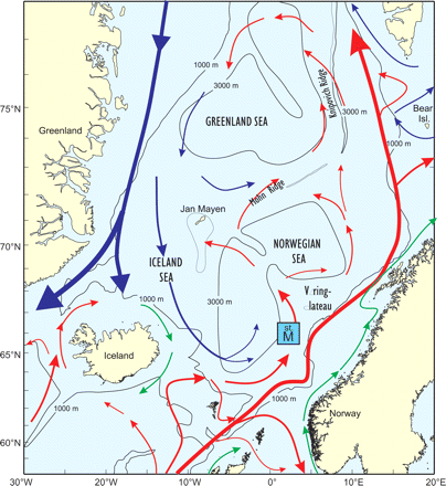
Bathymetry and main prevailing current systems in the Nordic seas.
Phytoplankton represents the primary trophic level in marine pelagic ecosystems, through which most of the biological material produced by photosynthesis is further channelled through the foodweb via grazing by zooplankton. The efficiency of this transfer depends strongly on the match between primary and secondary production. Because zooplankton acts as a link between phytoplankton on one hand, and fish and other organisms up the food chain on the other, the timing, intensity, and level of primary production are believed to be important factors for fish recruitment and growth. This link has recently been demonstrated for the eastern continental shelf of Canada (Platt et al., 2003). Because the Nordic seas are important feeding areas for commercially important fish stocks, enhanced knowledge of primary production and its variability in the area are important.
The Nordic seas cover a large area south and north of the Arctic Circle, on both sides of the Arctic Front. Therefore, phytoplankton is exposed to wide variations in physical forcing factors such as light, temperature, and nutrient supply, which controls growth. To estimate the annual primary production under such conditions is almost impossible mainly for logistical reasons that result in a scarcity of measurements. Nevertheless, through combining existing measurements in the Norwegian Sea, an annual rate of ∼80 gC m−2 y−1 has been estimated (Rey, 2004). Using estimates of nutrient depletion from Ocean Weather Station Mike (OWSM; 66°N, 2°E; for position, see Figure 2), it is assumed that some 60% of this is new production. However, in view of the strong grazing pressure in the Norwegian Sea, it is plausible to suggest that the assumed regenerated production must represent only a minimum level (Bathman et al., 1990). The actual regenerated production could easily be much higher (Rey, 2004). Annual production rates in the Greenland and Iceland seas are apparently comparable with those in the Norwegian Sea, i.e. a total production of ∼70 gC m−2 y−1 and new production some 55 gC m−2 y−1 (78%). However, it appears that the ratio of new to regenerated production varies with latitude, increasing from south to north (Rey et al., 2000). The highest rates of production in the Nordic seas are in the Norwegian Coastal Current, and they vary between 90 and 120 gC m−2 y−1, with new production rising from ∼50% of the annual production in the south to 70% in the north (Rey, 1981).

Mean (1981–2004) modelled annual depth integrated primary production (gC m−2 y−1) (left), and the Nordic seas with bathymetry and boxes (1–6), station M (cross) and the transects (a) Faeroe–Shetland, (b) Bear Island–Fugløya, (c) Fram Strait, and (d) Denmark Strait (right).
On a seasonal or annual basis, the net community production is assumed to approximate new production. Based on the analyses of oxygen flux to upper mixed layer, Skjelvan et al. (2001) estimated a net community production of 24 and 32 gC m−2 y−1, respectively, for two sections in the Norwegian Sea and 34 gC m−2 y−1 for the central Greenland Sea. Using a similar approach, Falck and Gade (1999) estimated a value of 25 gC m−2 y−1 for OWSM in the Norwegian Sea. Using a 1D ecosystem model for the Norwegian Sea, Haupt et al. (1999) report a total production of 90 gC m−2 y−1 and new production of 63 gC m−2 y−1 (70%). Finally, Broström (1997) reported total and new production of 180 and 59 gC m−2 y−1, respectively, from model simulations at OWSM.
Here, primary production in the Nordic seas was investigated using a coupled physical, chemical, and biological ocean model, the NORWegian ECOlogical Model system (NORWECOM) (Skogen et al., 1995; Skogen and Søiland, 1998). The model has been run for 24 years (1981–2004). In addition, a second run for 1997 has been performed to give a model estimate of new production. The simulated primary production estimates were compared with those from literature. Further, the interannual variability was studied to provide better insight on the dynamics of biological activity at a primary level within the Nordic seas, and its possible consequences for higher trophic levels.
Material and methods
NORWECOM is a coupled physical, chemical, and biological model system (Aksnes et al., 1995; Skogen et al., 1995; Skogen and Søiland, 1998), which can be applied to study primary production, nutrient budgets, and the dispersion of particles such as fish larvae and pollution. The model has been validated by comparison with field data in the North Sea/Skagerrak by, for example, Svendsen et al. (1996), Skogen et al. (1997, 2004), and Søiland and Skogen (2000).
The physical model
For the current study of the Nordic seas, NORWECOM was upgraded so that the physical model could be based on a new ice-ocean model system run at high spatial resolution for a multi-year simulation and validated against available observations (Budgell, 2005; Lien et al., 2006).
Ocean model component
The ocean model component is based on the Regional Ocean Modelling System (ROMS) version 2.1. ROMS is a 3D baroclinic general ocean model, the development of which is described in a series of papers (Song and Haidvogel, 1994; Haidvogel and Beckmann, 1999; Haidvogel et al., 2000; Shchepetkin and McWilliams, 2003, 2005). ROMS uses a topography-following coordinate system in the vertical that permits enhanced resolution near the surface and bottom (Song and Haidvogel, 1994). Orthogonal curvilinear coordinates are used in the horizontal. A spline expansion has been used for vertical discretization, which allows improved representation of the baroclinic pressure gradient (Shchepetkin and McWilliams, 2003), vertical advection, and vertical diffusion of momentum and tracers. ROMS has been designed from the ground up to run efficiently in both distributed (MPI) and shared (OpenMP) memory parallel computing environments, so allowing computationally intensive dynamic downscaling experiments to be conducted.
Ice model component
Large portions of the area of interest are ice-covered for much of the year. Therefore, it is important to include the effects of ice drift, melting, and freezing on the ocean fields. To accomplish this, a dynamic thermodynamic sea-ice module has been developed and coupled to the ocean model. The ice dynamics are based upon an elastic-viscous-plastic (EVP) rheology after Hunke and Dukowicz (1997) and Hunke (2001). The EVP scheme is based on a time-splitting approach whereby short elastic time-steps are used to regularize the solution when the ice exhibits nearly rigid behaviour. Because the time discretization uses explicit time-stepping, the ice dynamics are readily parallelizable, so computationally efficient. Employing linearization of viscosities about ice velocities at every elastic (short) time-step, as recommended by Hunke (2001), has the desirable property of maintaining the ice internal stress state on or in the plastic yield curve. That is, the ice deforms as a plastic material unless it is in a rigid state. Another desirable property of the Hunke (2001) linearization is that the EVP ice dynamics provide a good transient response to rapidly varying winds as well as to inertial and tidal dynamics, particularly in the marginal ice zone.
The ice thermodynamics are based on those of Mellor and Kantha (1989) and Häkkinen and Mellor (1992). Two ice layers and a single snow layer is used in solving the heat conduction equation. The snow layer possesses no heat content, but is, in effect, an insulating layer. Surface melt ponds are included in the ice thermodynamics. A molecular sublayer (Mellor et al., 1986) separates the bottom of the ice cover from the upper ocean. The inclusion of the molecular sublayer produces more realistic freezing and melting rates than if the ice-ocean heat flux is based purely on the temperature difference between the ice bottom and the upper layer of the ocean.
The chemical–biological model
The chemical–biological model is coupled to the physical model through the subsurface light, the hydrography, and the horizontal and vertical movement of the water masses. The prognostic variables are dissolved inorganic nitrogen, phosphorus, and silicate, two different types of phytoplankton (diatoms and flagellates), detritus (dead organic matter), diatom skeletals (biogenic silica), inorganic suspended particulate matter, and oxygen. The model is fully described by Skogen and Søiland (1998), but for completeness, a short review of the main processes is given in the Appendix.
The processes included are primary production, respiration, algal death, remineralization of inorganic nutrients from dead organic matter, self-shading, turbidity, sedimentation, resuspension, sediment burial, and denitrification. Phytoplankton mortality is given as a constant fraction (10% d−1), and is assumed to account also for zooplankton grazing which, in this context, is included as a forcing function. Particulate matter has a sinking speed relative to the water and may accumulate on the bottom if the bottom stress is below a certain threshold value; in like vein, resuspension takes place if the bottom stress is above a limit. Remineralization takes place in both the water column and the sediments. Parameterization of the biochemical processes and the exchange between the water column and sediment are taken from literature based on experiments in laboratories and mesocosms, or deduced from field measurements (Pohlmann and Puls, 1994; Aksnes et al., 1995; Gehlen et al., 1995; Lohse et al., 1995, 1996; Mayer, 1995).
Model set-up, forcing, and initialization
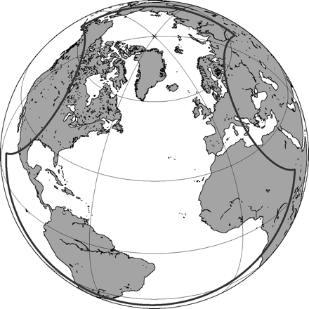
For our study, a model area that covers the North Atlantic (from 20°S) and the Arctic was used (Figure 3). A stretched spherical coordinate grid (Bentsen et al., 1999) is used in the horizontal, with the North Pole situated in central Asia and the South Pole situated in the Pacific Ocean west of North America. In the region of the Nordic seas, the horizontal resolution is ∼20 km. There were 30 generalized σ-coordinate(s) levels, stretched to increase vertical resolution near the surface and the seabed.
No tides were included in the simulation. The vertical mixing scheme employed was the LMD (Large et al., 1994) parameterization. The LMD scheme was used because it produces good agreement with observed mixed-layer behaviour in the deep ocean (Large and Gent, 1999). The incoming and outgoing fluxes were both set to 1 Sv, distributed uniformly across the two open boundary sections (outflow through the southern boundary, inflow through the Bering Strait). Zero normal gradients were specified for T and S, so that the only variations in these variables along the boundaries were attributable to atmospheric heat and salt (E–P) fluxes and vertical mixing. Zero normal gradients were also used at the open boundaries for all biochemical variables.
The atmospheric forcing was obtained from reanalysis of NCEP/NCAR data (Kalnay et al., 1996). Daily mean wind stress, and latent, sensible, downward short-wave radiative and net long-wave radiative heat fluxes were applied as surface forcing, after correcting for differences in model and NCEP surface conditions, such as in surface temperature and ice concentration. The flux corrections applied were developed by Bentsen and Drange (2000) and provide a feedback between the model surface temperature and applied heat fluxes, so minimizing problems with drift in model surface temperatures. Precipitation was taken from daily mean NCEP values. Snowfall was taken to be precipitation, corrected for snow density, when air temperature was <0°C. Evaporation was computed from the latent heat flux. River run-off was computed using the NCEP/NCAR reanalysis daily accumulated surface run-off values over land that were routed to ocean discharge points using the total run-off integrated pathways (TRIP) approach of Oki and Sud (1998). The hydrographs were modified for areas north of 60°N to account for permafrost hydrology and storage in snow cover.
The model simulation was started from 1 August 1980, initialized from fields from that date from a coarse resolution (50 km grid size) simulation of the North Atlantic and Arctic oceans for the period 1948–2002, as described by Budgell (2005). A time-step of 900 s was used for both the ocean internal mode and ice thermodynamics. A ratio of 30 was used between the ocean internal and external mode time-steps, and one of 60 was used between ice thermodynamic and dynamic time-steps. The physical model was run initially whereas the biochemical model was run in off-line mode, using 3D mean physical fields. The time-step of the biochemical model was 1 h.
The incident irradiation used in the biochemical model was modelled using a formulation based on Skartveit and Olseth (1986, 1987), using data for global daily downward short-wave radiation from the NCEP/NCAR reanalysis data set. The nutrient fields are re-initialized every 1 January using typical values for winter nutrients of Atlantic Water in the Norwegian Sea, 12.0, 5.5, and 0.8 µM of inorganic nitrogen, silicate, and phosphate, respectively (FR, unpublished data). Such a re-initialization avoids any drift in the nutrient fields, and will have minor effect on the results because the annual variations in winter nutrient concentration are no greater than ∼10% (Rey, 2004). The model is initialized with small amounts of algae (0.10 mgN m−3) for both diatoms and flagellates. Inorganic nitrogen is added to the system from the atmosphere (200 mgN m−2 y−1) (Anon., 1998), while there are no river nutrients.
Results and discussion
Our main objective has been related to the biological model because the physical results have been presented elsewhere (Lien et al., 2006). However, for reference purposes, an example of the circulation and temperature under different North Atlantic Oscillation (NAO) conditions is shown in Figure 4. Mean winter (December–March) temperature and currents 20 m deep for 1995 (high NAO) and 1996 (low NAO) are shown. The model clearly reproduces the large-scale patterns in the area (Figure 1), with a warm North Atlantic Current moving north along the Norwegian coast, and cold water moving south along the coast of Greenland on the western side. The figure also shows intensified currents under high NAO, compared with the situation in 1996 when, for instance, the West Spitsbergen Current was almost absent.
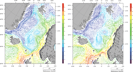
Mean modelled winter (December–March) temperature and currents 20 m deep for 1995 (high NAO) and 1996 (low NAO).
Figure 2 shows the mean (1981–2004) modelled annual depth integrated primary production (gC m−2 y−1). There are clear gradients, with highest production in the southeast and lowest in the northwest. This is consistent with the higher temperatures on the eastern side of the basin primed by the warm Northeast Atlantic Current, in contrast to the cold East Greenland Current coming from the Arctic (Figure 4). There is also clear evidence of topographic effects on production patterns, with more production over steep areas because of increased mixing bringing nutrients into the upper layers. The mean Norwegian Sea production is 79 gC m−2 y−1, agreeing with previous estimates of 80 gC m−2 y−1, with levels highest in the Norwegian Coastal Current (80–120 gC m−2 y−1). At OWSM, the modelled production is 74 gC m−2 y−1, with new production of 55% (1997 value), also in accord with previous estimates (60%). The mean Iceland and Greenland Sea annual production is estimated at 70 and 65 gC m−2 y−1, respectively (70 gC m−2 y−1 in the literature). There is also a slight increase in the ratio of new to regenerated production with latitude, from ∼70% in the Iceland Sea to 75% (1997 values) in the Greenland Sea, slightly below previous estimates (mean ∼78%).
The mean annual production in the whole Nordic seas was 73 gC m−2 y−1. The highest value was in 1982 (81 gC m−2 y−1) and the lowest in 1986 and 1987 (66 gC m−2 y−1). This gives a 20% difference in total phytoplankton biomass between the years of extreme primary production. However, there are large spatial differences in this interannual variability. In the Greenland Sea, the variability is almost 50% (mainly the consequence of different ice conditions between years), whereas it is <20% over the deeper part of the Norwegian Sea. Looking at the interannual variability at OWSM, there are very large differences varying from a minimum of 61 gC m−2 y−1 in 1984 to a maximum in 1985 of 91 gC m−2 y−1.
The timing of the spring phytoplankton bloom depends strongly on the physical conditions, especially the development of the upper mixed layer. Time-series observations from OWSM have shown that the time at which the bloom reaches its peak can vary by as much as 5–6 weeks from year to year, controlled mainly by the stability in the area (W. Melle, Institute of Marine Research, Bergen, pers. comm.). Also, as a rule, there seems to be top-down control, so that strong grazing pressure of zooplankton, especially in the pre-bloom phase, will result in a later and smaller bloom peak. Late blooms, therefore, favour more efficient transfer of energy from phytoplankton to zooplankton. Observations indicate that the average time of the peak spring bloom is 21 May (mean for 1991–2003), and that the maximum observed chlorophyll-a concentration during the same period was barely >3 mg Chla m−3 (Rey, 2004). Comparing these data with simulated ones, the average time of the peak bloom at OWSM is on 15 May in the model, and the maximum chlorophyll-a concentration is about 4 mg Chla m−3. However, the modelled time at which the bloom reaches its peak only varies by ∼2 weeks from year to year compared with the 5–6 weeks from observations. The main reason for this is probably the use of a constant zooplankton-grazing rate in the model, which is unable to simulate the observed top-down controlled grazing pressure.
Comparing the date of peak chlorophyll-a between model and observations (Figure 5) gives a positive correlation (r = 0.67). Focusing on the years of very late/early chlorophyll-a maxima, there is general agreement between model and data of late production in 1996 and 2001, and early production in 1998 and 2002. Best fit is in the more recent years, whereas the greatest discrepancy is in 1991, when the model indicates a very early chlorophyll-a maximum, while the data show a very late one.
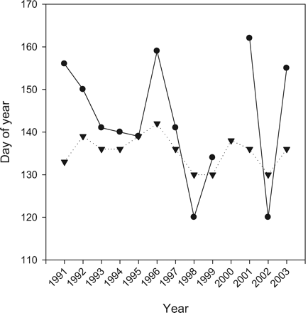
Measured (dots) and modelled (inverted triangles) day number of peak chlorophyll-a concentration at Ocean Weather Station Mike (OWSM). Note that no value was measured in 2000.
Although there is a positive relationship between the timing of the bloom, there is no relationship (r = −0.07) between the level of the measured and the modelled chlorophyll-a maximum. This can be explained from the closing of the model where a constant death and grazing rate are used, and no mechanism is included to simulate a top-down controlled system, a late phytoplankton bloom giving a lower phytoplankton biomass because of stronger grazing pressure from zooplankton. With the present formulations, the model instead gives a positive relationship between day number and modelled chlorophyll-a maximum, because of a higher sea surface radiation during a later bloom.
Dividing the Nordic seas into a number of boxes (Figure 2), the relationship between primary production in different areas can be investigated. The best correlation (r = 0.89) is between modelled annual primary production in Box 1 (the Greenland Sea) and the overall mean Nordic seas production. The correlation between Box 3 (deeper part of the Norwegian Sea) and the overall mean is also high (r = 0.77). There is a weak relationship between Box 6 and the downstream Boxes 3–5 (r = 0.50, 0.35, 0.49, respectively). Finally, there is a positive relationship (r = 0.53) between Boxes 1 and 3, and a negative relationship (r = −0.51) between Boxes 2 and 4. All these values are listed in Table 1. An interesting observation is that there is only a slight correlation between primary production at OWSM (situated on the edge between Box 3 and 5; Figure 2) and Boxes 3 and 5. This probably reflects the fact that these areas represent different water masses with different patterns in their primary production. This is especially true for Box 5, which includes both Atlantic and Coastal waters. It is well known that, although OWSM mostly represents Atlantic water, waters of coastal origin occasionally reach OWSM. These results support the common knowledge that a single measurement point in the ocean is not a good approximation for the biological variability of a whole oceanic area.
Correlations between modelled annual primary production in the different boxes, 1981–2004.
| Box . | Area 2 . | Area 3 . | Area 4 . | Area 5 . | Area 6 . | OWSM . | Mean . |
|---|---|---|---|---|---|---|---|
| Box 1 | 0.35 | 0.53 | 0.08 | −0.26 | −0.14 | 0.08 | 0.89 |
| Box 2 | 0.36 | −0.51 | −0.15 | 0.03 | −0.20 | 0.43 | |
| Box 3 | 0.03 | 0.13 | 0.50 | 0.19 | 0.77 | ||
| Box 4 | 0.42 | 0.35 | 0.13 | −0.04 | |||
| Box 5 | 0.49 | 0.36 | 0.13 | ||||
| Box 6 | 0.36 | 0.45 | |||||
| OWSM | 0.19 |
Primary production depends on light, temperature, available nutrients, and the development of the upper mixed layer. The variability of the modelled primary production can therefore be explained from variations in the modelled fields, and changes in the atmospheric forcing of the model. The NAO is one of the major modes of variability of the northern hemisphere atmosphere, so can be used as a proxy for atmospheric conditions over large areas. It is particularly important in winter, when it exerts a strong control on the climate. The modelled primary production has been compared with the NAO computed from the monthly difference between the normalized sea level pressure between Ponta Delgada, Azores and Stykkisholmur, Iceland (Hurrell, 1995). This comparison gives clear evidence of atmospheric control of primary production, with different patterns dependent on area. Using the mean NAO for the first 6 months of the year as a proxy for the large-scale atmospheric control, there is a positive relationship (r = 0.46) with the NAO (high NAO giving high annual production) in the Iceland Sea (Box 2). On the eastern side of the Nordic seas, there is negative dependence. At the Barents Sea entrance (Box 4), r = −0.46 between the NAO and modelled primary production, and with Box 5 r = −0.63 (Figure 6). In the last three boxes (1, 3, and 6), the existence of a simple atmospheric control is weaker, even if there are some evidence of a relationship between NAO in early spring (February and March) and the modelled primary production in Boxes 1 and 3. Such a dependence can be explained as preconditioning of the production through stabilization in early spring and is partly confirmed by data from OWSM that indicate the presence of a relationship between the timing of the pre-bloom and the level of new production (FR, unpublished data). The different relationships between eastern and western side are consistent with the way the NAO controls the weather system, with high NAO giving stronger storms crossing the Atlantic Ocean on a more northerly track along with enhanced mixing and destabilization of the upper layers on the eastern side. A high NAO will, by contrast, lead to a cold and dry climate over Greenland and less mixing on the western side.

Relationship between NAO (dots) month 1–6 and annual primary production (gC m−2 y−1) in Box 5 (inverted triangles).
The modelled ice coverage varies significantly between years, independent of the winter NAO. As ice coverage varies from year to year, so too does subsurface light, limiting phytoplankton growth. Maximum ice extent varies from year to year, but is normally found in March in the Nordic seas. Using 15% ice concentration in March as a threshold for modelled ice cover, the annual ice coverage varies between 0.66 and 1.43 (mean 1.04) million km2. This agrees with data from NASA's Goddard Space Flight Center (mean 0.87, r = 0.57), and comparing the modelled ice coverage in March with annual primary production in the Greenland Sea, there is a clear negative dependence (r = −0.74, Figure 7), as there is for the whole Nordic seas (r = −0.63).
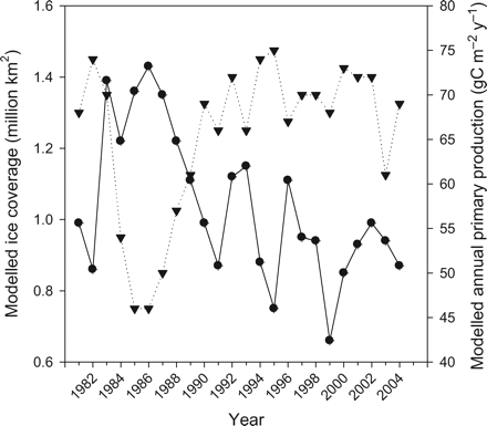
Relationship between modelled ice coverage (million km2) in March in the Greenland Sea (dots) and the modelled annual primary production (gC m−2 y−1) in Box 1 (Greenland Sea) (inverted triangles).
Transport in the Nordic seas, which is driven by at least two main forcing mechanisms namely wind stress at the sea surface and densification by cooling at high latitudes, will also depend on variation in the NAO. For example, increased wind forcing associated with a high NAO index results in an increased volume transport in the slope current (Orvik et al., 2001; Orvik and Skagseth, 2003). The resulting transport of different water masses will again redistribute the available nutrients for primary production in both time and space. Therefore, a strong link between modelled transport and primary production can be expected, and is found, in most areas. The strongest relationship was found with the Greenland Sea (Box 1), where the correlation between the annual mean modelled transport into the area (southwards) through the Fram Strait and the modelled annual primary production was r = 0.85. With the strong link between the mean Nordic seas production and Greenland Sea production (Table 1), the annual transport through the Fram Strait also has a strong positive correlation (r = 0.74) with mean Nordic seas production (Figure 8). On the other hand, there is negative correlation (r = −0.50) between transport and the annual production in Box 4 (Barents Sea entrance), consistent with the different response to the NAO on the eastern and western sides of the Nordic seas. In like manner, there are reasonable relationships between the other boxes (except for Box 6) and transport in the Fram Strait.
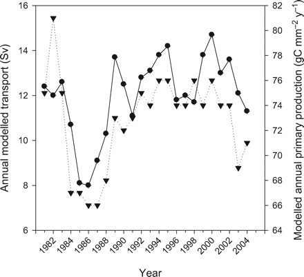
Relationship between annual modelled transport through the Fram Strait (1 Sv = 106 m3 s−1) (dots) and modelled mean annual primary production in the Nordic Seas (gC m−2 y−1) (inverted triangles).
At first sight, a relationship between transport in the Fram Strait and primary production in other parts of the Nordic Seas is unexpected, but because the volume transport into the Nordic seas has to balance the transport out of the area, there is a link between transport through different sections. In fact, there is positive correlation between the modelled annual transports through the Fram Strait and the Denmark Strait (r = 0.73) and the Faeroe to Shetland section (r = 0.77), and between the latter two (r = 0.52). In contrast, inflow to the Barents Sea through the Bear Island to Fugløya section is almost independent of other flows (see Figure 2 for the positions of the transects). These results are partly confirmed by another model study (Nilsen et al., 2003) that suggests a tight link between the inflow in the Faeroe–Shetland Channel and the outflow through the Denmark Strait, and a study by Skagseth et al. (2004), who found that the flow along the slope from the Irish–Scottish shelf towards the Fram Strait wase forced by anomalies in sea level pressure (resembling the NAO pattern), with no phase lag. Finally, Ingvaldsen et al. (2004) showed that the inflow to the Barents Sea is controlled mainly by local winds. This would explain the relationship between transport in the Fram Strait and primary production, relationships that also could have been expressed in terms of transport through the other sections.
Concluding remarks
The present version of the model represents a tool for gaining new insight into the complex dynamics between physics and biology in the ocean, an insight that is hard to achieve through measurements only. However, limitations have to be taken into account when interpreting the results. The horizontal resolution is a limiting factor with respect to correct simulation of, for example, nearshore and mesoscale processes. Also, the NCEP forcing used in the simulations was coarse (spatial resolution ∼2°) and the cloud cover fraction was too low, necessitating correction of the radiative fluxes using cloud data from the International Satellite Cloud Climatology Project (ISCCP).
A further weakness is the upper closing of the model at the zooplankton level using a constant grazing rate. Work is in progress to make a two-way coupling with an IBM for Calanus finmarchicus, which represents about 25% of the biomass and 80% of the secondary production in the area. Preliminary results indicate that such a coupling would strengthen top-down control. A first effect of this is seen in an increase in the concentration of chlorophyll-a during the after bloom, in better agreement with observations (e.g. Rey, 2004).
This work in our opinion represents a step towards better understanding of the Nordic seas ecosystem. In terms of the input of biological energy and its subsequent transfer, the most important single process is the annual phytoplankton spring bloom. This is because annual zooplankton production is tightly linked to phytoplankton production, so that timing, duration, and the level of the spring bloom are important factors for the efficiency of further transfer of energy to higher trophic levels. This was demonstrated by Svendsen et al.(in press), who showed how recruitment of Arcto–Norwegian cod was linked to primary production in the Barents Sea. It is also well known that climate can control growth and recruitment at higher trophic levels (Holst et al., 2004; Melle et al, 2004; Ottersen et al., 2006). Through the close connection between climate and phytoplankton production demonstrated here, a possible mechanism for how climate can be an important control on available biological material in the foodwebs is suggested.
Acknowledgements
We thank Vidar S. Lien (IMR) for making Figure 4 on the circulation and temperature under different NAO conditions. The work was supported by the Norwegian Research Council (NRC) within projects ADAPT (152906/120) and CLIMAR (155889/S30), and through the NRC Programme for Supercomputing through a grant of computing time.
References
Appendix
A short overview of the biochemical model is given below. A complete description is given in Skogen and Søiland (1998), and it can be downloaded from http://www.imr.no/~morten/norwecom.
Incident radiation


This model gives a climatological light formulation as a function of the area dependent constants ax,…, fx. An interpolation technique for these constants has been developed to include data for total daily irradiance, and the daily downward solar radiation flux from the NCEP/NCAR reanalysis data set has been used. The formulae are valid when the solar elevation is >5°, but they have been used for all solar elevations.
Light in the water column


A similar formulation is given for the direct light, Idir(x,y,z,t), by substituting Rdif with Rdir and μ with cos(ϕ), where ϕ is the zenith angle of the direct light in the water column.
Primary production
The concentration of chlorophyll in the system is affected by the production of the algae, their death and by respiration. As zooplankton is not included in the model, the grazing is (very roughly) included in the constant death rate of 10% per day.


All these expressions refer to diatoms. Analogous formulations are used for flagellates, except that silicate is not rate limiting for them. The biological parameter values were chosen according to independent validation against mesocosm experiments (Aksnes et al., 1995).
Oxygen
The oxygen concentration is affected by the primary production, respiration, and remineralization of detrital matter. The amount of oxygen released by primary production is proportional to the amount of inorganic nitrogen consumed, and is given by a constant (Redfield ratio). The same ratio for oxygen consumption is used for respiration and remineralization process. The ratio is based on the assumption that inorganic nitrogen is converted from nitrate to organic matter and vice versa. For the fraction of nitrogen that is denitrified in the sediments, somewhat less consumption takes place.


