


Abstract
Background: Despite the growing chronic disease burden in low- and middle-income countries, there are significant gaps in our understanding of the financial impact of these illnesses on households. As countries make progress towards universal health coverage, specific information is needed about how chronic disease care drives health expenditure over time, and how this spending differs from spending on acute disease care.
Methods: A 19-year panel dataset was constructed using data from the Kagera Health and Development Surveys. Health expenditure was modelled using multilevel regression for three different sub-populations of households: (1) all households that spent on healthcare, (2) households affected by chronic disease and (3) households affected by acute disease. Explanatory variables were identified from a review of the health expenditure literature, and all variables were analysed descriptively.
Findings: Households affected by chronic disease spent 22% more on healthcare than unaffected households. Catastrophic expenditure and zero expenditure are both common in chronic disease-affected households. Expenditure predictors were different between households affected by chronic disease and those unaffected. Expenditure over time is highly heterogeneous and household-dependent.
Conclusions: The financial burden of healthcare is greater for households affected by chronic disease than those unaffected. Households appear unable to sustain high levels of expenditure over time, likely resulting in both irregular chronic disease treatment and impoverishment. The Tanzanian government’s current efforts to develop a National Health Financing Strategy present an important opportunity to prioritize policies that promote the long-term financial protection of households by preventing the catastrophic consequences of chronic disease care payments.
Chronic disease-affected households spend 22% more on healthcare costs than unaffected households.
Predictors of healthcare expenditure differ between chronic disease-affected and -unaffected households.
Analysis of health expenditure over a 19-year panel reveals heterogeneous and household-dependent spending patterns.
Introduction
The burden of chronic disease is increasing in low- and middle-income countries (LMICs), driven by infectious diseases including HIV and tuberculosis (TB) as well as a growing burden of non-communicable diseases (NCDs). Chronic infectious disease and NCD burdens also compound each other in a variety of ways. First, co-morbidities exist between infectious diseases and NCDs including HIV and cardiovascular disease, and TB and diabetes (Young et al. 2009). Second, interactions between NCDs, infectious disease and poverty have been documented; diabetes-affected adults in Tanzania reported the need to make difficult choices between paying for their own care or that of their children with infectious diseases (Kolling et al. 2010).
Existing literature well describes the financial impact of chronic disease in high-income countries, whereas a small but increasing number of studies has begun to examine this impact in LMICs. Context-specific research is necessary because the financial impact of chronic illnesses is likely to be different in LMIC settings, where healthcare costs fall more heavily on households and individuals than on governments and insurance schemes (Kankeu et al. 2013). The economic impact of chronic disease on households operates through a combination of direct and indirect costs. Direct costs include both the costs of care itself (consultation, hospitalization, medication, etc.) and the costs associated with accessing care such as the cost of transportation. Indirect costs may be incurred whether or not an individual seeks treatment and consist primarily of lost income due to illness (McIntyre et al. 2006; Kankeu et al. 2013).
A review of studies that examined the household economic burden of HIV/AIDS, TB and malaria in LMICs found that these illnesses impose regressive cost burdens on patients and their families. Furthermore, costs associated with HIV and TB care were likely to reach a catastrophic level, and poorer households struggled to cope with these costs. A recent study of patient and household TB costs from eight African countries found that pre-diagnostic costs alone often reached catastrophic levels. Despite the value of these cross-sectional analyses examining the economic burden of chronic infectious diseases, there remains a lack of findings drawn from longitudinal data (Russell 2004; Ukwaja et al. 2012).
A recent review of 49 studies examining the financial impact of chronic diseases (primarily NCDs) in LMICs identified a heavy, regressive financial burden arising from medicine costs and a lack of insurance coverage for NCDs. The review also identified the following substantial gaps in the literature:
There is little information from the sub-Saharan Africa region.
Many studies use data collected from individuals identified by convenience sampling, which is likely to bias results and conclusions.
Few studies compare predictors of expenditure between chronic and acute illnesses.
There are no analyses of panel data, and a time dimension may be crucial to understanding the evolution expenditure over time (Kankeu et al. 2013).
There is a growing attention to the necessity of financial risk protection for individuals and households, and this protection underpins the movement towards universal health coverage that is on-going in many LMIC settings, including Tanzania (Mtei et al. 2014). Catastrophic out-of-pocket (OOP) health expenditure is a common measure of the impact of a lack of financial risk protection. These data are typically presented as an incidence of households experiencing such expenditure at a point in time (Saksena et al. 2014). Importantly, this indicator—the use of which is necessitated by the cross-sectional nature of many datasets—is unable to signify the impact of catastrophic expenditure on a household over time, further necessitating the inclusion of a time dimension when considering financial risk due to catastrophic healthcare payments.
Tanzania is a sub-Saharan African country classified as low-income by the World Bank. In 2013 Tanzania’s population was 49.3 million, and life expectancy in 2012 was 62 years for females and 60 years for males (World Bank Group 2013). OOP payments are the primary source of health financing. Available insurance schemes are fragmented, limiting achievable cross-subsidization and risk pooling. Health insurance is, however, mandatory in the formal employment sector, with the National Health Insurance Fund covering public employees and the Social Health Insurance Benefit of the National Social Security fund providing coverage for private sector employees. The Community Health Fund scheme exists for informal sector workers (Mills et al. 2012; Mtei et al. 2014).
In Tanzania, NCDs account for 31% of adult deaths, with cardiovascular disease and diabetes causing 9% and 5% of all deaths, respectively. High blood pressure—the leading risk factor for NCDs globally—is also common in Tanzania, affecting 31.6% of male adults and 29.4% of female adults. In 2013, the HIV prevalence rate amongst adults aged 15–49 was 5.0% (UNAIDS 2013; World Health Organization 2014).
The data used in this analysis were collected from Kagera, the northwestern region of Tanzania. Approximately half of the population is aged 0–14, and 5% is older than 65 (De Weerdt 2010). Kagera was an early epicentre of HIV/AIDS, with some of the first cases detected in 1983 originating in this region. The urban area of the Bukoba district was particularly affected, with HIV prevalence peaking at 24% in 1987. Prevalence remained lower in rural areas and decreased across the entire region throughout the 1990s. This study aims to compare the level and predictors of expenditure on healthcare between chronic disease-affected (CDA) and unaffected (CDU) households in this region using 19-year panel data.
Methods
Dataset and variable construction
The data used in this analysis come from the Kagera Health and Development Surveys (KHDS), a longitudinal survey started by the World Bank in 1991. Specifically, 6353 respondents forming roughly 900 households were selected from a stratified random sample of the 1988 census. The sample was stratified on the basis of (1) agro-climatic zone and (2) adult mortality rate (to account for the high prevalence of HIV/AIDS in this region of Tanzania) (World Bank Development Research Group 2004). Resurveys of the original respondents were conducted in 2004 and 2010, including tracing of those who had moved out of the region (De Weerdt et al. 2010). This panel had a very low attrition rate compared with other longitudinal surveys, with 93% of original respondents re-contacted in 2004, and 88% re-contacted in 2010 (Litchfield and McGregor 2008). Appendix 1 contains an in-depth explanation of the survey data and key expenditure variables. Ethical clearance was not required for this study as it is a secondary analysis of publicly available data.
Acute illness was defined as an illness experienced in 4 weeks prior to the household interview that lasted less than 6 months; chronic diseases were defined as existing for 6 months or more. Chronic disease therefore can capture both NCDs and other long-run illnesses, such as HIV and TB. Additional verification questions were asked for each case of illness, including questions regarding the duration, symptoms, and diagnosis of the illness. Examination of self-reported illness perception and practitioner diagnoses for acute and chronic illnesses via tabulation showed that these verification questions resulted in accurate disease classification.
These data are analyzed using longitudinal regression models. Household-level explanatory variables were selected for inclusion on a theoretical basis and from an examination of the health expenditure literature for LMIC settings. Table 1 lists the selected variables, their composition and descriptive statistics.
Descriptive statistics for household-level health expenditure and independent variables
| Variable | Description | Mean | SD | Min | Max |
|---|---|---|---|---|---|
| Healthexp | Household level expenditure on healthcare (expressed in 2010 USD) | 34.46 | 279.10 | 0 | 11 566.27 |
| ConsumptionExp | Household level consumption expenditure (expressed in 2010 USD) | 1457.29 | 1318.43 | 25.63 | 19 087.90 |
| Chronic | Number of adults reporting chronic disease | 0.38 | 0.64 | 0 | 5 |
| Nonchronic | Number of adults reporting non-chronic disease | 0.89 | 0.92 | 0 | 8 |
| Headwork | Household head works (binary) | 0.59 | 0.49 | 0 | 1 |
| Headmale | Household head is male (binary) | 0.76 | 0.42 | 0 | 1 |
| Headsingle | Household head is unmarried (binary) | 0.33 | 0.47 | 0 | 1 |
| HeadAge | Age of the household head | 44.27 | 16.87 | 16 | 99 |
| HeadEducation | Years of education of the household head | 6.97 | 2.87 | 0 | 21 |
| Tobaccoexp | Household expenditure on tobacco in the past 2 weeks (2010 USD) | 0.59 | 1.25 | 0.004 | 20.86 |
| Overweight | Number of overweight individuals (BMI > 25) | 0.20 | 0.47 | 0 | 5 |
| Size | Household size | 5.38 | 3.12 | 0 | 36 |
| Adults | Number of adults in the household | 2.28 | 1.17 | 0 | 16 |
| Elderlymen | Number of elderly men older than 65 years | 0.09 | 0.29 | 0 | 2 |
| Elderlywomen | Number of elderly women older than 65 years | 0.12 | 0.34 | 0 | 3 |
| Insurance | Number of individuals covered by an insurance scheme | 0.14 | 0.49 | 0 | 7 |
| Private | Household use of private clinics, including traditional healers (binary) | 0.16 | 0.36 | 0 | 1 |
| Urban | Urban location of household (binary) | 0.17 | 0.38 | 0 | 1 |
| Education | Average years of schooling of household members | 5.75 | 2.32 | 0 | 17 |
| Age | Average age of household members | 24.17 | 11.89 | 7.25 | 94 |
Smoking and obesity are two risk factors for chronic disease development and are controlled for with variables that indicate household tobacco expenditure and the number of overweight individuals (Abegunde and Stanciole 2008).
Total consumption expenditure (TCE) was selected as an indicator of the economic status of households, due to the low levels of formal sector employment in LMIC settings (Deaton 1997; Howe et al. 2012). TCE and health expenditure are annualized, and health expenditure includes the costs of hospitalization, outpatient care, medicines and transportation. Catastrophic health expenditure was determined by calculating the proportion of the non-food TCE spent on healthcare, with >40% defined as catastrophic expenditure. This is a commonly used measure as the non-food portion of TCE captures the capacity to pay after meeting subsistence needs, and it has been used in a variety of health expenditure studies in LMICs, including Tanzania (Xu et al. 2003; Chuma and Maina 2012; Brinda et al. 2014).
The three expenditure-related variables (health expenditure, TCE and tobacco expenditure) were log-transformed to meet the normality assumption of the multilevel growth model that was fit to the data. There were no zero-value TCE expenditures, and tobacco expenditure data were either non-zero or missing; zero health expenditure values were omitted as missing during log transformation. To minimize truncation caused by the zero health expenditure values, health expenditure was set to missing instead of zero for all households lacking any form of illness. All expenditure variables were adjusted for inflation using a KHDS-specific Fisher price index that corrects prices both temporally and spatially (World Bank Development Research Group 2012). Unless otherwise noted, all values are expressed in 2010 USD (1 USD = 1409.27 Tanzanian Shillings) (The World Bank 2014).
All analyses were carried out using Stata Version 12. For descriptive analyses comparing health expenditure means, we used the non-parametric Mann–Whitney test to test for statistical significance due to the non-normal distribution of health expenditure.
Regression modelling
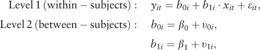
There are several challenges associated with modelling health expenditure. Such data are typically skewed with a right-hand tail, and there are a large number of ‘zero’ value responses from non-spenders. There are also challenges associated with this particular dataset that are not addressed by standard modelling techniques such as two-part models and generalized linear models (GLMs). First, because the households have repeated measurements for the same variables over time, there is a high degree of autocorrelation between the separate household-level observations in the dataset. Second, the panel is unbalanced; there are uneven gaps in the data (10 years between 1994 and 2004, and 6 years between 2004 and 2010). Finally, household chronic disease presence and the number of disease cases at the household level are not necessarily consistent at all time points in the panel; in other words, households may report chronic disease at one or more time points, but not all time points in the panel.
To address these challenges, a multilevel growth model was selected to examine health expenditure over time. These models incorporate random subject effects (in this case, the subject is the household) to account for the effects of subject characteristics that influence their repeated observations, in addition to a population-level fixed effects specification. We estimated three random effects specifications, which represent (1) individual household variance around the population slope, (2) household variance around the population intercept (together representing between-household variance) and (3) within-household variation. Because time is treated as a continuous independent variable, subjects are not required to have data at every time point, which simultaneously increases statistical power while avoiding bias that would result from the analysis of complete cases only (Hedecker 2004).
Three different household classifications were used for all analyses: (1) all households with nonzero health expenditure, (2) CDA households and (3) households affected by acute disease, referred to here as CDU households.
Results
Descriptive analyses
Across the panel, 31% of households reported one or more cases of chronic disease. In all but 2 years (1991 and 1993), health expenditure was higher in CDA households compared with CDU households (Table 2). Across all years, mean health expenditure was $39.63 (SD: 287.91) for CDA households and $32.63 (SD: 255.70) for CDU households (P < 0.0001).
Mean health expenditure (inflation adjusted and expressed in 2010 USD)
| Household type | 1991 (SD) | 1992 (SD) | 1993 (SD) | 1994 (SD) | 2004 (SD) | 2010 (SD) |
|---|---|---|---|---|---|---|
| All spending households | $39.92 | $42.06 | $60.81 | $66.88 | $13.48 | $38.01 |
| (329.46) | (333.64) | (538.78) | (580.39) | (22.71) | (75.66) | |
| CDA households | $36.18 | $58.78 | $42.44 | $85.42 | $16.12 | $42.69 |
| (54.20) | (542.42) | (171.77) | (647.06) | (22.13) | (102.93) | |
| CDU households | $44.83 | $34.63 | $59.79 | $34.30 | $11.91 | $30.76 |
| (396.39) | (153.42) | (536.92) | (81.50) | (18.96) | (45.71) |
Across the panel, health expenditures represented 2.74% (SD: 0.18) of TCE for CDA households, compared with 2.54% (SD: 0.12) in CDU households (P = 0.0034). There is a notable decrease in health-related spending between years 1994 and 2004, and an increase between 2004 and 2010 (Table 2 and Figure 1).
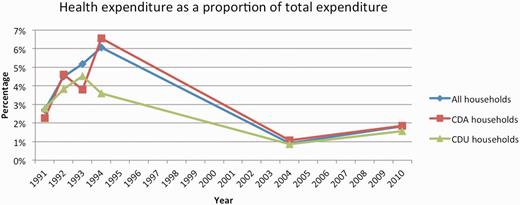
Health expenditure over the 19-year panel, expressed as a percentage of total consumption expenditure and stratified by household disease status.
From 1991 to 1994, 3.16% of CDA households spent catastrophically, compared with 4.18% of CDU households. Levels of catastrophic spending increased substantially for both sub-populations of households in 2004 and 2010, although the increase for CDA households was greater (Figure 2). 12.70% and 19.91% of CDA households spent catastrophically in 2004 and 2010, respectively. Across the panel, 7.54% of CDA households spent catastrophically, compared with 6.68% of CDU households.
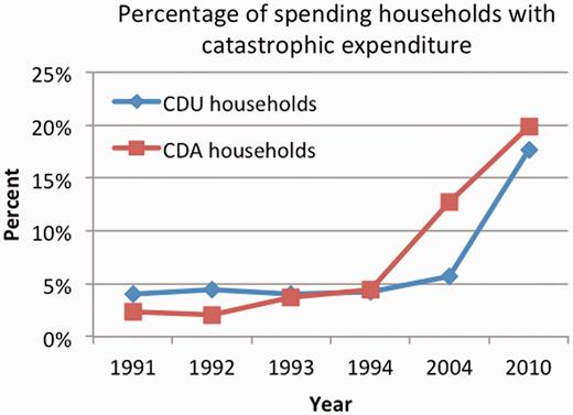
Rates of catastrophic spending (defined as >40% of non-food consumption expenditure).
Rates of non-spending on healthcare among CDA households were low during the years 1991–94 and increased substantially during years 2004 and 2010 (Table 3).
Percentage of CDA households with zero health expenditure
| 1991 | 1992 | 1993 | 1994 | 2004 | 2010 | |
|---|---|---|---|---|---|---|
| % of CDA households with zero health expenditure | 0.00 | 1.36 | 0.62 | 1.35 | 6.32 | 14.76 |
| 1991 | 1992 | 1993 | 1994 | 2004 | 2010 | |
|---|---|---|---|---|---|---|
| % of CDA households with zero health expenditure | 0.00 | 1.36 | 0.62 | 1.35 | 6.32 | 14.76 |
The lowest wealth quintile had the highest number of ill individuals, and the lowest rates of health expenditure and catastrophic spending. Quintiles 4 and 5 have the highest rates of health and catastrophic spending (see Table 4).
Illness, health spending and catastrophic spending by quintile
| Quintile | N | n with illness | n spenders | % of ill that spend | n catastrophic spending | % catastrophic spending |
|---|---|---|---|---|---|---|
| 1 | 1853 | 1411 | 1243 | 88 | 65 | 5 |
| 2 | 1853 | 1326 | 1234 | 93 | 74 | 6 |
| 3 | 1853 | 1275 | 1199 | 94 | 121 | 10 |
| 4 | 1853 | 1245 | 1203 | 97 | 149 | 12 |
| 5 | 1853 | 1217 | 1170 | 96 | 163 | 14 |
Regression analyses
Three multilevel growth models were fit to model the predictors of health expenditure in the three populations of households. The first model examines the predictors of health expenditure in the ‘population of households with non-zero health expenditure’, regardless of chronic/non-chronic disease status (Table 5). The second model examines predictors of health expenditure among ‘CDA households’ (Table 6). The third model examines predictors of health expenditure among ‘CDU households’ (Table 7).
Regression results for spending households
| logHealthExp | Coefficient | P |
|---|---|---|
| Time | 0.0192551 | 0.000 |
| Nonchronic | −0.0041958 | 0.497 |
| Chronic | −0.0063695 | 0.470 |
| Headwork | 0.012882 | 0.233 |
| Headmale | −0.035051 | 0.356 |
| Headsingle | −0.0773257 | 0.002 |
| HeadAge | 0.0014355 | 0.178 |
| HeadEducation | 0.0017139 | 0.716 |
| logTobaccoexp | −0.0022767 | 0.695 |
| Overweight | 0.0030682 | 0.831 |
| Size | 0.0656502 | 0.000 |
| Adults | −0.0048474 | 0.552 |
| Elderlymen | −0.0382192 | 0.276 |
| Elderlywomen | 0.0377922 | 0.160 |
| Insurance | 0.0562016 | 0.081 |
| Private | −0.023205 | 0.215 |
| Urban | 0.1177726 | 0.087 |
| logConsExp | 0.0149477 | 0.227 |
| Education | 0.0003221 | 0.959 |
| Age | −0.0027624 | 0.012 |
| Constant | 8.967644 | 0.000 |
| Random effects specifications | ||
| Specification | Value | P |
| SD(slope) | −2.321 | 0.000 |
| SD(intercept) | 0.376 | 0.000 |
| SD(household) | −2.392 | 0.000 |
Notes: N = 1454; Number of groups = 804.
Regression results for CDA households
| logHealthExp | Coefficient | P |
|---|---|---|
| Time | 0.0036426 | 0.561 |
| Chronic | 0.0008877 | 0.941 |
| Nonchronic | −0.0117211 | 0.167 |
| Headwork | 0.0146282 | 0.203 |
| Headmale | −0.296144 | 0.002 |
| Headsingle | −0.2859161 | 0.000 |
| HeadAge | 0.000945 | 0.648 |
| HeadEducation | 0.0176821 | 0.018 |
| logTobaccoexp | 0.0032634 | 0.553 |
| Overweight | −0.023758 | 0.058 |
| Size | 0.0659472 | 0.000 |
| Adults | 0.0243677 | 0.009 |
| Elderlymen | 0.1674903 | 0.001 |
| Elderlywomen | 0.01559 | 0.546 |
| Insurance | 0.03413 | 0.707 |
| Private | 0.0243348 | 0.143 |
| Urban | 0.2361526 | 0.085 |
| logConsExp | 0.002934 | 0.846 |
| Education | −0.0106249 | 0.153 |
| Age | −0.003232 | 0.048 |
| Constant | 9.498247 | 0.000 |
| Random effects specifications | ||
| Specification | Value | P |
| SD(slope) | −2.869 | 0.000 |
| SD(intercept) | 0.138 | 0.000 |
| SD(household) | −3.820 | 0.000 |
Notes: N = 472. Number of groups = 372.
Regression results for CDU households
| logHealthExp | Coefficient | P |
|---|---|---|
| Time | 0.0122553 | 0.035 |
| Nonchronic | −0.0026051 | 0.705 |
| Headwork | 0.0110865 | 0.342 |
| Headmale | −0.0804274 | 0.058 |
| Headsingle | 0.0179105 | 0.496 |
| HeadAge | 0.0012965 | 0.312 |
| HeadEducation | 0.0089433 | 0.094 |
| logTobaccoexp | 0.0005803 | 0.929 |
| Overweight | 0.0185591 | 0.261 |
| Size | 0.0633386 | 0.000 |
| Adults | 0.0021816 | 0.816 |
| Elderlymen | −0.0443497 | 0.297 |
| Elderlywomen | −0.0202822 | 0.587 |
| Insurance | −0.0664356 | 0.058 |
| Private | −0.0136477 | 0.523 |
| Urban | 0.2299636 | 0.017 |
| logConsExp | 0.0035163 | 0.796 |
| Education | 0.002802 | 0.702 |
| Age | −0.0016441 | 0.186 |
| Constant | 9.092241 | 0.000 |
| Random effects specifications | ||
| Specification | Value | P |
| SD(slope) | −2.518 | 0.000 |
| SD(intercept) | 0.325 | 0.000 |
| SD(household) | −2.633 | 0.000 |
Notes: N = 982. Number of groups = 623.
For the population of spending households, time and household size are strong positive predictors of expenditure, whereas an unmarried household head and increasing household age are strong negative predictors of expenditure. An urban location and a higher number of insured individuals weakly but positively predict expenditure.
For the population of CDA households, time is not a significant predictor of expenditure. Household size, the number of adults and the number of elderly men in a household are strong positive predictors of expenditure, whereas a male household head and an unmarried household head are strong negative predictors of expenditure. The education level of the household head positively predicts expenditure, whereas the average household age negatively predicts spending. Finally, urban location is a weak positive predictor of expenditure, whereas the number of overweight individuals is a weak negative predictor of expenditure.
For the population of CDU households, time was a positive predictor of expenditure; thus, CDA households were the only population for which expenditure does not appear to increase over time. A male household head negatively predicts expenditure, whereas the education level of the head positively predicts expenditure; however, these effects are weaker in CDU households compared with CDA households. In contrast, urban location is a strong predictor of expenditure in these households, whereas this effect was more modest for CDA households. Finally, household size is a strong positive predictor of expenditure, whereas the number of insured individuals is a weak negative predictor of expenditure.
Finally, the three random-effects specifications were highly significant in all three models, demonstrating considerable variation in both the level of expenditure and the change in expenditure by households over time.
Discussion
The finding that households affected by chronic diseases experience a greater OOP expenditure burden (in this study, 22% higher) confirms other studies from LMIC contexts (Russell 2004; McIntyre et al. 2006; Chuma et al. 2007). This higher level of expenditure might be explained by the long-term nature of treatment for chronic illness, and also by the fact that most CDA households (73.9%) also experienced one or more instances of acute illness, which suggests that households might spend to meet healthcare needs for several household members. Alternatively, the individual experiencing chronic disease could simultaneously be experiencing an acute (or chronic) comorbidity. The observation that catastrophic expenditure was more common in households within the higher economic quintiles (12% and 14% in the top two quintiles compared with 5% and 6% in the bottom two quintiles) suggests that better-off households tend to spend a larger portion of household resources on healthcare than poorer households; this aligns with a finding that was observed in the context of Asian countries (van Doorslaer et al. 2007). Alternatively, poorer households might not seek care due to the direct and indirect costs of care-seeking, which could explain the observation of lower healthcare expenditure in the bottom two quintiles. The increase in both catastrophic- and zero-expenditure beginning in 2004 remains an important topic for further examination.
Catastrophic expenditure rates for both CDA and CDU households were also higher than the recently reported Tanzanian national average of 2%; this could be a result of the HIV/AIDS burden in the Kagera region, which was substantially larger compared with other parts of Tanzania (Mtei et al. 2014).
Across the 19-year panel, time was a significant positive predictor of expenditure for CDU households, suggesting a general increase in healthcare expenditure over time. However, time was not a significant predictor of expenditure for CDA households. This suggests that CDA households are unable to maintain high levels of chronic disease care expenditure over time. An increase in the number of adults in a household reporting chronic or non-chronic illness did not significantly increase health expenditure. This suggests that households might lack the resources to increase health expenditure when there are multiple cases of either chronic or acute disease.
In all three models, urban household location was a positive predictor of expenditure. This suggests that individuals residing in rural areas might be less likely to receive treatment. Alternatively, these individuals might be receiving more cost-efficient care from dispensaries or health centres (instead of at costlier hospitals), or care that is subsidized through community-based programmes (Saronga et al. 2014). Among all spending households, the number of household members covered by an insurance scheme positively predicted health expenditure (P = 0.081). This aligns with the findings of other studies (Ruger and Kim 2007; Abegunde and Stanciole 2008) and suggests that in the Tanzanian context insurance schemes may offer some—but not complete—protection from incurring OOP expenditure. Another possible explanation lies within the earlier observation that increasing cases of illness do not correlate with increasing expenditure. It is therefore possible that the presence of increasing numbers of insured individuals allows households to use financial resources to access care for those not covered by an insurance scheme. An examination of individual-level expenditure and insurance status by household would be necessary to further evaluate this idea.
Demographic characteristics of the household head are more important to predicting health expenditure in CDA households than in CDU households. For example, the presence of a male household head and/or an unmarried head negatively predicts expenditure (P = 0.002 and P = 0.000), whereas education level of the head positively predicts expenditure (P = 0.018). However, in CDU households, only the male head and education level trends are conserved, and even then only at the P < 0.1 level. These results suggest that decisions regarding expenditure might be made differently for chronic vs acute diseases. Although the head of the household has previously been identified as playing a key role in determining other household members’ access to healthcare, it appears that this role might be influenced when the decisions relate to accessing care for a chronic condition (Anderson and Bartkus 1973; Okunade et al. 2010; Fang et al. 2013).
The number of adults and the number of elderly men in a CDA household are also strong positive predictors of health expenditure, which aligns with the idea that these individuals are more likely to develop a chronic condition (most likely an NCD) and incur health expenditure as a result. Accordingly, these two variables were not significant predictors of expenditure in CDU households.
Although TCE is positively associated with health expenditure, this trend was not statistically significant in any of the three models. The economic status of a household has repeatedly been shown to be a significant positive predictor of health expenditure (Andersen and Newman 1973; Parker and Wong 1997; Abegunde and Stanciole 2008; Okunade et al. 2010; Fang et al. 2013). When the log of non-food consumption expenditure was used in place of TCE, this measure of income became a positive predictor of health expenditure with greater statistical significance (not shown). These results suggest that non-food consumption expenditure, which represents a household’s capacity to pay, is a better measure of the economic status of a household than TCE for this setting.
Finally, the random-effects parameters that estimate between household variance and within household variance represent an important finding of this study. These effects were highly significant in each of the three models, and indicate that there is a significant degree of household variation around the population-level health expenditure growth curve. Taken together, these results suggest that CDA households—and indeed, all households in Kagera that have non-zero health expenditure—have highly heterogeneous health expenditure patterns over time. Although the fixed effect regression results indicate that these expenditure patterns are determined in part by household characteristics, such as size, economic status, urban location, insurance coverage, and demographic characteristics of the household head, these parameters suggest that expenditure patterns are also highly household-specific, especially when considered over an extended period of time.
Finally, Tanzania has several health system characteristics that are common to other LMIC settings. These include a relatively fragmented financing system shaped by a history of colonial rule and structural adjustment, and a high proportion of OOP payments (McIntyre et al. 2008). It is therefore likely that the household spending patterns presented here are also relevant to CDA households in similar settings. However, it is also worth noting that this dataset showed higher rates of catastrophic spending (7.54% among CDA households and 6.68% in CDU households) than the Tanzanian national average of 2%, which might be explained in part by the historically high rates of HIV/AIDS in this region of the country (Mtei et al. 2014).
Although every attempt has been made to make best use of the available secondary data, this study has a number of known limitations. First, incurred costs are likely to vary by chronic disease, medicines tend to be the largest component of treatment costs, and the level to which these costs might be subsidized is likely to vary by disease. For example, this region has experienced significant scale-up in HIV treatment programmes; meanwhile, the cost of insulin treatment for diabetes remains significant. Costs of palliative care in sub-Saharan Africa have also been shown to be significant (Harding and Higginson 2005; Kankeu et al. 2013). The large proportion of individuals lacking a formal diagnosis of their condition (39.2% across the panel) limited the potential to accurately control for the effects of specific diseases. The reported prevalence of chronic disease could also be underestimated due to a reliance on self-reported information; low levels of diagnosis, lack of awareness of disease progression and stigma surrounding certain illness such as HIV could have limited self-reporting (Binnendijk et al. 2012; Walker et al. 2013).
The large proportion of zero health expenditure responses results in truncation of the dependent variable, a common challenge in analysing health expenditure data (Deaton 1997). However, log transformation of the health expenditure variable was necessary because multilevel growth models rely on a normality assumption that, if violated, produces biased confidence intervals and hypothesis tests (Bernier et al. 2011). There is limited information in the literature regarding the behaviour of multilevel growth models under the presence of censoring and truncation (Sweeting and Thompson 2012). Across this dataset, 4.63% of health expenditure responses were equal to zero, which is low compared with other settings (Okunade et al. 2010). Meanwhile, the annualized nature of the health expenditure data could result in a ‘scaling up’ of acute expenditure; this might overestimate levels of health-related spending, and should be kept in mind when interpreting these data. Furthermore, the addition of time-varying covariates into the multilevel models might better model any potential lagged effects of chronic disease on household health expenditure, which might better address the endogenous nature of health status to health expenditure (Rous and Hotchkiss 2003; Hedecker 2004). Additional examination of the increasing levels of zero expenditure and catastrophic expenditure over the panel is also warranted.
It is also worth discussing the decrease in health-related expenditure between 1994 and 2004 (Table 2 and Figure 1); we see two possible explanations for this. First, questions regarding health related spending were moved from the health-related section of the survey to the individual expenditure portion of the survey in 2004. The specific wording of the questions was also changed slightly. Second, the decrease could be a reflection of the evolution in the HIV burden that occurred during the gaps between the data collection points in the 1990s and the 2000s. For example, the development of HIV programmes providing subsidization of medicines and services between the 1990s and 2010 could explain the relative decrease between these time points, as could the corresponding increase in life expectancy due to antiretroviral availability and an associated decrease in palliative care costs, which are known to be high.
Finally, the dataset lacks information on monetary and/or asset transfers to households that is consistent across all years of the panel; data surrounding household splits resulting from illness-related financial stress are also lacking. Therefore, no conclusions can be drawn regarding how households might cope with the financial burden of chronic disease. This remains an important topic for future examination.
Conclusion
The results of this study have revealed the financial burden of CDA households. These households appear unable to sustain high levels of expenditure over time. Predictors of expenditure are highly heterogeneous and household-dependent, and differ between CDA and CDU households. Our analysis of the KHDS panel demonstrates the importance of analyzing the financial risk of catastrophic health expenditure with a time dimension. The findings of this study, concurrent with the Tanzanian government’s present efforts to develop a health financing strategy, demonstrate the importance of policies that provide long-term financial protection of Tanzanian households experiencing chronic illness.
Funding
This work was supported by the Marshall Scholarship Program.
Conflict of interest statement. None declared.
References
Appendix 1: KHDS survey data description
The KHDS survey series includes a comprehensive household questionnaire as well as several additional community questionnaires. Data collected at the household level include information regarding consumption, income, assets, household amenities, business activities, time allocation of individuals, and individual health, education and anthropometric information. One of the community questionnaires collected detailed food and non-food price information from various local stalls and marketplaces. These were used to construct a KHDS-specific Fisher price index to adjust for inflation across the panel.
The KHDS strategy for the follow-up survey rounds (2004 and 2010) was to track and re-interview individuals rather than households due to the dynamic nature of a household over time. As a result, the first time point contains roughly 900 households, whereas the 2010 data point represents over 3300.
Description of key expenditure variables
TCE includes:
Food expenditure.
Consumption of home production, including food; business outputs; livestock; and any other non-food consumption.
Alcohol and cigarette consumption.
Consumption of non-food items including rent, tax, clothing, jewellery, fuel and services.
Sent remittances.
Expenditure/consumption of wage income that was received in-kind.
The components of TCE had recall periods ranging from 2 weeks to 1 year depending on the nature of the item. TCE was expressed as an aggregate variable assembled by the KHDS team for download with the rest of the data, and it is expressed as an annualized value adjusted for inflation.
Health expenditure was collected for both living and deceased individuals, and was collected in two different manners for comparison and verification purposes by the KHDS team at the beginning of the panel:
Section 18A of the survey collected expenditure information for either the past 12 or 6 months in two broad categories: medicines and other medical services.
Section 6 (the Health section) asked questions that linked spending to episodes of acute illness occurring in the past 4 weeks, including medicines, hospitalization, outpatient costs and transportation. There was an additional ‘global’ question for all expenditure on chronic conditions that occurred in the past 4 weeks.
When comparing the two methods, there were very few instances (across 1991–94, less than 3% overall) in which the summed expenditure from Section 6 exceeded that from Section 18 (as would be expected due to the shorter recall period of the questions in Section 6). For those few individuals, annual health expenditure was summed from Section 6. For the remaining majority of individuals, annual health expenditure was set as the sum of the items in Section 18 plus the transportation costs collected in Section 6A. In a manner similar to the TCE variable, health expenditure was summed for all individuals in a household to arrive at an annual household total (World Bank Development Research Group 2004).
Changes in survey structure and implementation across the panel
Below we describe changes that occurred in the survey structure, design and/or implementation that occurred in the two re-survey rounds of 2004 and 2010. We describe these changes for both TCE and health expenditure, which are the critical expenditure variables used in our analysis. The majority of the changes were global section order and structure changes.
TCE-related changes from 1991–94 to 2004:
In 2004, individual expenditures originally assessed in Section 18B were moved to section 15C and instead assessed at the household level. These included household supplies such as fuel. This original Section 18B was then dropped.
In 2004, some individual expenditures originally assessed in Section 18A were moved to the Household Annual Expenditure level (Section 15B in 2004).
In 2004, Section 8 became the Individual Expenditure section. Some of the individual expenditure questions had changes in recall periods and wording.
In 1991–94, there was a unique fishing section that in 2004 was moved to the non-farm self-employment section.
In 2004, crop-related questions were further divided into questions for each specific crop sub-type.
In 2004, questions regarding income and expenditures for enterprises were combined into the same category (they were in separate categories in 1991–94).
In 2004, consumption of home-grown fruits and vegetables was combined; in 1991–94, data were collected for each item.
Health expenditure-related changes from 1991–94 to 2004:
In 2004, health expenditures were assessed only in the Individual Expenditures section instead of in the health section. This Individual Expenditure section was moved to Section 8 from the original Section 18.
The exact wording of the health-related expenditure questions changed slightly in order to capture transportation costs (originally in Section 6, the health section), and the recall period was set at 12 months (Beegle et al. 2006).
In 2010, KHDS shifted to an electronic survey collected on handheld computers. Price data, originally a community questionnaire, were collapsed into the household questionnaire.
TCE-related changes from 2004 to 2010:
A few individual expenditure items, including expenditures on sports, cinemas and gambling were dropped.
Questions surrounding the sale of crops were moved to a new Land section.
2004 questions regarding farm inputs were dropped.
In 2010, detailed questions regarding expenditure and income relating to enterprises were dropped.
In 2010, household expenditure items were updated (e.g., to include a category on mobile phone and internet expenditures).
Health expenditure-related changes from 2004 to 2010:
Illness associated expenses for household members who died in the past 12 months were dropped, as were funeral and other death-associated expenses for these members (De Weerdt et al. 2010).
Full descriptions of survey design and implementation are available in the Basic Information Documents cited above.
Appendix 2: Regression modelling
First, it is worth noting that there are a variety of methods that can be used to address the challenges of modelling health expenditure data, and there is considerable debate as to which models are best suited for various circumstances (Buntin and Zaslavsky 2004). Here, we describe some limitations to standard two-part models and GLMs that we considered while choosing an approach to the model health expenditure data for this panel.
Two-part models separately model (1) the probability of spending on healthcare and (2) the level of spending conditional on nonzero expenditure (Duan et al. 1983). The second part usually utilizes a transformed expenditure or cost variable that is then re-transformed for interpretation. However, a smearing factor must be used in the event that the error term is not normally distributed, and in some cases heteroscedasticity in the error term may still result in the incorrect estimation of expenditure despite application of the smearing factor correction (Duan 1983; Buntin and Zaslavsky 2004).
GLMs are another option that use a link function to model the mean and variance on the original scale of the dependent variable (Nelder and Wedderburn 1972). However, GLMs are more likely to give imprecise estimates in the event of a mean or variance function misspecification, as they have weaker model assumptions when compared with alternatives such as the two part model and ordinary least squares (OLS) regression (Buntin and Zaslavsky 2004).
The additional challenges associated with this particular dataset that were mentioned in the Methods section (autocorrelation, the unbalanced panel and inconsistent chronic disease presence), along with the additional insight offered by estimating household-dependent random effects in addition to the population-level fixed effects led us to choose a multilevel regression model (Stata command xtmixed).
