


SUMMARY
With the deployment of high quality and dense permanent seismic networks over the last 15 yr comes a dramatic increase of data to process. In order to lower the threshold value of magnitudes in a catalogue as much as possible, the issue of discrimination between natural and anthropogenic events is becoming increasingly important. To achieve this discrimination, we propose the use of a convolutional neural network (CNN) trained from spectrograms. We built a database of labelled events detected in metropolitan France between 2020 and 2021 and trained a CNN with three-component 60 s spectrograms ranging frequencies from 1 to 50 Hz. By applying our trained model on independent French data, we reach an accuracy of 98.2 per cent. In order to show the versatility of the approach, this trained model is also applied on different geographical areas, a post-seismic campaign from NW France and data from Utah, and reaches an accuracy of 100.0 and 96.7 per cent, respectively. These tests tend to hypothesize that some features due to explosions compared to earthquakes are widely shared in different geographical places. In a first approach, we propose that it can be due to a contrast in the energy balance between natural and anthopogenic events. Earthquake seismic energies seem to be more continuous as a function of frequency (vertical bands features in a spectrogram) and conversely for explosions (horizontal strips).
1 INTRODUCTION
Studying low magnitude earthquakes allows us to better understand natural seismic activity, especially in stable continental regions where it is challenging to explain the occurrence of earthquakes under slow strain-rate conditions. Before 2000s, most of seismic stations operated in triggered mode, recording only events that exceeded an operator-defined detection threshold, while most of present-day stations continuously record the ground motion. This evolution comes at the cost of an increase in the processing capabilities but interestingly offers the possibility to reprocess ‘old’ data set with new methods to detect events with lower signal-to-noise ratio (SNR), and consequently lower magnitudes seismic events. Denser seismic station networks and high sensitivity modern instruments improve our understanding of global and local seismicity over the last decade (e.g. Levandowski et al. 2018; Beucler et al. 2021). As an illustration of the evolution of the seismic data volume, the size of the IRIS DMC (Incorporated Research Institutions for Seismology Data Management Center) archive has grown from 25 terabytes (TB) in 2005 January to 800 TB in 2022 January. In metropolitan France, the number of stations from the FR network (RESIF 1995) has increased from 56 in 2005 January to 157 in 2020. This massive flow of global seismic data implies an important human and temporal cost for the data processing and creation of a catalogue of seismic events (e.g. detection, picking of seismic phases and discrimination of events).
One of the major challenges in developing an event catalogue, is the discrimination between natural (tectonic events) and anthropogenic events (caused by human activity, as quarry blasts or military explosions). In metropolitan France, instrumental seismicity is mostly characterized by low magnitude earthquakes (Cara et al. 2015). The deployment of new permanent stations since mid-2018 (Beucler et al. 2021; Doubre et al. 2021; Larroque et al. 2021; Sylvander et al. 2021) has conducted to an increase in the number of detected natural and anthropogenic seismic events. However, metropolitan seismicity is now dominated by the detection of anthropogenic events (for instance, see fig. 7 in Beucler et al. 2021), originating from quarry blasting, military training operations or underwater mine explosions along the French coast (e.g. Favretto-Cristini et al. 2020). It is therefore necessary to find an efficient solution to help the discimination of all these low magnitude seismic events.
Several semi-automatic or automatic approaches have already been developed using, for example, the amplitude ratio between seismic phases (Baumgardt & Young 1990; Dysart & Pulli 1990; McLaughlin et al. 2004; Tibi et al. 2018; Pyle & Walter 2019; Wang et al. 2020), using spectral content (Gitterman et al. 1998; Allmann et al. 2008), or studying the coda (Su et al. 1991; Koper et al. 2016). These types of methods are highly dependent of the SNR and of the epicentral distance (some seismic phases may not be visible at very short distances). However, extracting these information from large data sets can be quite time consuming and the choice of these parameters can be seen as relatively subjective.
To overcome these problems, such as finding relevant features to classify the data, machine learning tools can be implemented. In the last few years, these approaches were widely used for the detection of events (Yoon et al. 2015; Ross et al. 2018; Mousavi et al. 2020), automatic picking of seismic phase on raw data (Pardo et al. 2019; Woollam et al. 2019; Zhu & Beroza 2019), but also for signal classification using features extracted directly from the data (Del Pezzo et al. 2003; Meier et al. 2019; Renouard et al. 2021), or relying on deep neural networks (Li et al. 2018; Linville et al. 2019). In the latter, training algorithms with a sufficiently large database allow thoses programs to recognize, like humans, natural objects and to make expert-level decisions.
Among those algorithms, convolutional neural networks (CNNs, a nonlinear classifiers which is a subcategory of neural networks) can achieve high-performance recognition and outperform simple linear classifiers. Linville et al. (2019) show that using spectrograms with a frequency content between 1 and 20 Hz as input for a CNN allows to achieve high predictive capability in distinguishing natural from anthropogenic events. If the frequency range used by Linville et al. (2019) is well suited for local to regional moderate magnitude events, in cases of low magnitudes events (Ml < 2) occuring in low attenuation medium (such as Armorican Massif, Mayor et al. 2018) a significant part of the recorded signal reaches frequencies up to 50 Hz. We thus propose to extend the spectrogram to frequencies larger than 20 Hz in order to take into account as much as possible the high-frequency spectral content. An additionnal constraint of the algorithm chosen in Linville et al. (2019) is the requirement of P-wave picking before the discrimination. By randomly selecting the beginning of the windows studied, we want to overcome this problem and apply the method directly after the detection step. CNNs can moreover automatically extract discriminative features from training data. One of the objectives of this study would be to verify whether these features deduced during training, on a specific geographical region, can be generalized to other regions.
In Section 2, we describe the CNN and the data set used to train it. Three different applications are presented in Section 3 which illustrates the versatility of the proposed approach. To this end, we used 3 datasets not used for training. These are composed of events located in different geographical areas: Metropolitan France, the United States and a local study in NW France. Finally, in Section 4, we discuss the performance of our discimination tool and the implications for decision support for discrimination between natural and anthropogenic events.
2 METHOD
2.1 Targets
The main objective of this paper is to describe an alternative discrimination of natural and anthropogenic seismic events, which inherently means low-to-intermediate magnitudes. At the present time, this classification is generally done by experienced analysts. Among criteria used to discriminate seismic events, the most widely used are the source parameters of the events (location, time of origin and magnitude) and the characteristics of the waveforms. Quarry blasts and explosions are generally observed between 9 a.m. and 6 p.m. during working days, whereas natural events can occur at any time of the day and night.
However, some configurations can make discrimination more challenging. For instance, a natural event occurring near the surface and/or near a quarry, can induce signals with characteristics similar to quarry blasts and will very likely be tagged as ‘anthropogenic event’ by an analyst. Low magnitude events produce signals with a low SNR, so differentiation can be complicated. In addition, with the increase in the amount of detections, due to the densification of station networks, we are dealing with a larger diversity of waveforms and the distinction between natural and anthropogenic events is becoming increasingly complex and time consuming.
To illustrate this diversity, Fig. 1 presents eight examples of natural and anthropogenic events (traces and spectrograms) labelled by the French National agency BCSF-RéNaSS (Bureau Central Sismologique Français—Réseau national de surveillance sismique), after visual inspection. Among them, five are natural events and three are anthropogenic events. The most striking difference between the two categories is the amplitude ratio between P and S waves. For natural events (Figs 1a, b, d, f and g) this ratio is generally lower than 1.0 while it almost equals to 1.0 for explosions (Figs 1c, e and h). On the spectrograms (right-hand panels of Fig. 1) of the natural events, we can clearly see two arrivals with a strong energy packet associated to the S-wave arrival that forms a vertical band that affects the whole frequency range. For the anthropogenic events, energy is generally confined to lowest frequencies and forms horizontal strips. Spectrograms thus seem to bear sufficient ‘visual’ information to help us to discriminate natural from anthropogenic events. Examples for marine explosions and shallow earthquakes are shown in Fig. S1 (Supporting Information).
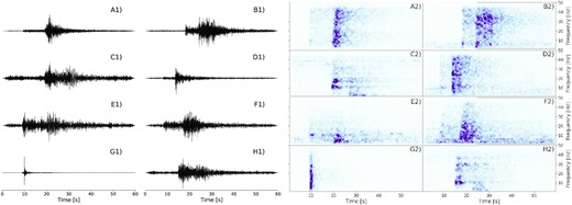
Examples of five natural events (A, B, D, F and G) and three anthropogenic events (C, E and H), recorded by the FR network stations, with the associated spectrograms. The seismic signals correspond to the normalized raw data of the vertical component. The spectrograms are normalized by their maximum. All technical details of the events are in Table S1 (Supporting Information).
To achieve high classification performances, and given the fact that spectrograms are images, we have chosen to implement an automatic classifier with a CNN which are ‘machine learning’ approaches that were proven to be particularly efficient for image recognition.
2.2 Convolutional neural network
The discrimination of the two families of signals is achieved through a supervised learning algorithm based on a CNN. A CNN allows to extract discriminating features through the successive application of hierarchical filters of defined size. The choice of implemented CNN architecture is guided by those presented in the literature (e.g. Linville et al. 2019; Meier et al. 2019) and by standard choices made in deep learning (e.g. Géron 2019). The first layers correspond to the convolution layers which, thanks to filters of a defined size, allow the extraction of features from the input. Then, these features are implemented in fully connected layers where the number of neurons per layer varies. We tested about 10 different architectures by varying the number of convolution layers (from 3 to 4 layers), the number of filters (16 to 128) and the number of neurons in the fully connected layers (80, 128 and 256). The training accuracy (see definition in Section 2.4) of these different architectures ranges from 92.83 to 95.63 per cent.
The CNN with the best performances is composed of four convolution layers with respectively 18, 36, 68 and 68 filters for each layer and three fully connected layers (Table 1). We apply a 2 × 2 ‘max-polling’, between each convolution layer, to allow a subsampling by keeping only the maximum values. The final layer of the neural network is the output layer that indicates the probabilities obtained with the ‘softmax’ activation function (Fig. 2). The coefficients of the filters and the weights of the fully connected network are jointly optimized during the training process to maximize the discrimination performance. As input to this CNN, we use normalized spectrograms of size 237 × 50 × 3, corresponding to time (T) × frequency (F) × channels. The process to obtain these spectrograms is explained in the next section.
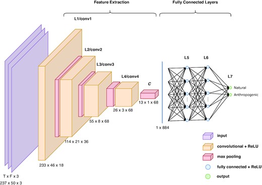
The CNN architecture. The input of the array corresponds to the three-component spectrograms of size 237 × 50 (time × frequency). The L1–L4 layers extract the characteristics thanks to the application of a series of filters allowing the downsampling of the matrix. This feature extraction leads to the C matrix which is flatten to be injected in the fully connected layers. The CNN output corresponds to the two probabilities for the classes: natural and anthropogenic. See Table 1 for more technical details on the CNN.
Technical details of the CNN. conv: convolution, fc: fully connected and ReLU: rectified linear unit. Convolution layers from L1 to L4 and fully connected layers from L5 to L7.
| L1 | L2 | L3 | L4 | L5 | L6 | L7 | ||
|---|---|---|---|---|---|---|---|---|
| Layer Type | conv | conv | conv | conv | fc | fc | fc | |
| Number of filter/neuron | 18 | 36 | 68 | 68 | 80 | 80 | 2 | |
| Filter size | (5,5) | (3,3) | (3,3) | (2,2) | ||||
| Activation | ReLU | ReLU | ReLU | ReLU | ReLU | ReLU | softmax |
2.3 Training data set
The CNN is trained on a data set composed of elements tagged with two classes: natural and anthropogenic (quarry blast and explosion). To generate this database, we use the BSCF-RéNaSS bulletin between 2020 January 01 and 2021 June 01, for events with Ml ≤ 3. This bulletin is restricted to metropolitan France extended outside its exclusive economic zone of 20 km. For each selected event, the three-component seismic waveforms are collected at stations from FR network for which at least a P-wave pick is documented in the bulletin.
The data set is composed of 30 054 natural events records (corresponding to 5172 natural events) and 25 549 anthropogenic events records (4877 anthropogenic events) at 136 permanent stations. To have a balanced database between the two classes, we have randomly selected, using a uniform distribution, 25 000 records in each class. This provides a set of 50 000 records that correspond to 5016 and 4788 natural and anthropogenic events, respectively. The consequences of different choices for the training dataset are discussed in Section 4.2.
Fig. 3 shows the geographical distribution of the stations used to train the CNN. The majority of the stations are grouped in the mountainous areas (Alps in zone B and Pyrenees in zone C). In the rest of France, the stations are more evenly distributed.
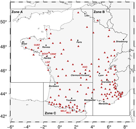
Geographical distribution of the stations used for the training of the CNN and the end-2021 French data application (136 permanent stations of the FR network). The Metropolitan France has been divided into three subsections. These geographical zones A, B and C are discussed in Section 4. The number of stations per zone is shown in Table 2. The seven named stations are used as examples for Fig. 1.
Fig. 4 shows the geographic distribution of natural and anthropogenic events in the database. We observe areas with a high concentration of natural events, such as the Pyrenees (zone C), the Alps and the Upper Rhine Grabben (zone B, Table 2). In comparison, in the Armorican Massif and the Massif Central (zone A), known as stable continental areas, fewer scattered natural events are observed. As expected, we have a few or no earthquakes in the Aquitaine Basin and the Paris Basin, which coincides with the general seismicity of these regions (Cara et al. 2015). For anthropogenic events, the distribution of quarries is very heterogeneous and also related to the geology and tectonic history of the regions. In zone A, 84.4 per cent of the events correspond to anthropogenic events, whereas for zones B and C, the ratios are 48 per cent and 31 per cent, respectively (Table 2).
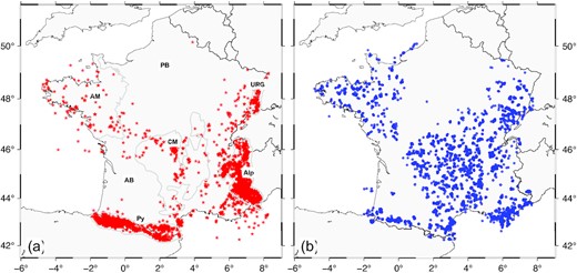
Geographic distribution of training, validation, and test databases composed of 9804 events detected between 2020-01-01 and 2021-06-01 and labelled by the BSCF-ReNaSS. (a) 5016 natural events are represented by the red stars. The main French geological regions are contoured by the grey lines: PB: Paris Basin, URG: Upper Rhine Grabben, AM: Armorican Massif, CM: Central Massif, AB: Aquitaine Basin, Alp: Alps and Py: Pyrenees. (b) 4788 anthropogenic events (quarry blasts and explosions) are represented by the blue circles.
Partition of the data set.
| Zone A | Zone B | Zone C | Total | |
|---|---|---|---|---|
| Natural events | 255 | 2612 | 2149 | 5016 |
| Anthropogenic events | 1407 | 2415 | 966 | 4788 |
| Records | 11 126 | 22 818 | 16 056 | 50 000 |
| Stations | 40 | 62 | 34 | 136 |
| Zone A | Zone B | Zone C | Total | |
|---|---|---|---|---|
| Natural events | 255 | 2612 | 2149 | 5016 |
| Anthropogenic events | 1407 | 2415 | 966 | 4788 |
| Records | 11 126 | 22 818 | 16 056 | 50 000 |
| Stations | 40 | 62 | 34 | 136 |
Waveforms are sampled at 100 sps (samples per second) and are sliced into 60 s windows. This window size limits the source-station distance used for discrimination to about 400 km which is consistent with our choice to focus on Ml ≤ 3 event. To mitigate the use of a priori information on the P-wave arrival and to make the CNN less sensitive to picking errors or phase mislabelling, we impose that the window starts randomly between 5 and 20 s before the P-wave pick. Indeed, depending on the focal mechanisms, the SNR or the method used [(for instance STA/LTA, e.g. Allen 1982) or template matching (e.g. Gibbons & Ringdal 2006)], detection time can indeed correspond to P or S-wave onset. This method does not require an exact and reliable choice of the P-wave onset time.
To standardize the data given to the CNN, waveforms are detrended, tapered (Hann window, 5 per cent of the total window) and filtered with a 2 Hz high-pass Butterworth filter (four-corner, two passes). Spectrograms are computed for 1 s sliding windows with 75 per cent overlap. We end with 237 time windows for which we compute their discrete Fourier transform between 1 and 50 Hz for the three components of the seismogram. For each seismogram, that is, each source-station couple, we thus obtain 237 × 50 × 3 elements matrices (time × frequency × channels).
2.4 Training results
True Positive (TP) is the number of natural events correctly classified by the CNN and False Negative (FN) represents the number of natural events classified as anthropogenic. False Positive (FP) is the number of anthropogenic events classified as natural and True Negative (TN) represents the number of anthropogenic events correctly classified by the CNN.
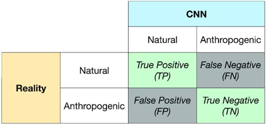
Example of a confusion matrix. Each cell of a confusion matrix contains a performance estimate of the CNN. In our case ‘Positive’ means Natural and conversely ‘Negative’ for Anthropogenic. The term ‘Reality’ means what the National agency BCSF-RéNaSS tagged as Natural and Anthropogenic. If the CNN gives exactly the same results as the Reality, only the main diagonal has non-zero percentage values.
Since the accuracy (1) is the ratio of the sum of all the true predictions over the amount of all possible predictions, it indicates whether the discrimination is correct. The precision (2) indicates how the algorithm is relevant for the discrimination of what is named ‘Positive’ (in our case, Natural). When the precision is high, it means that the majority of the positive predictions of the model are correct. The recall (3) quantifies the ratio of positive class predictions over all the actual positive classes. When the recall is large, it means that the majority of positive only elements are well classified. The F1-score (4) is a weighted average of precision and recall. This score thus accounts for both false positives and negatives.
The classifier achieved high scores with a training accuracy of 95.63 per cent. The score is computed using all elements independently of the event they are associated with, which is called a station-level prediction. It is possible to obtain an event prediction by combining all the elements at the station-level that correspond to the same event, it is called a network-level prediction. As a first approach, for a given event, a linear average of all station-level probabilities defines the probability at network level that leads to the event-based classification.
On the ‘validation’ data set (10 per cent of the database, i.e. 5000 records), the final model reaches an accuracy of 94.76 per cent at the station-level and of 95.11 per cent at the network level. The recall of natural and anthropogenic events is 93.58 and 96.58 per cent, respectively. The model incorrectly identifies 6.42 per cent of the natural events and 3.42 per cent of the anthropogenic events, thus, it is more likely to correctly predict the class of anthropogenic events. Finally, on the ‘test’ data set (10 per cent of the database, i.e. 5000 records), the model reaches an accuracy of 94.68 per cent at the station level and of 95.3 per cent at the network level.
3 VARIOUS DISCRIMINATIONS USING A UNIQUE TRAINED MODEL
To illustrate the relevance of the scheme chosen for the CNN and the versatility of our trained model, we apply it on three different case studies, none of them were used to train it: (i) a data set composed of events detected in metropolitan France for 5 months, (ii) a revisit of the events detected in the United States, mainly in Utah, and recorded by the University of Utah Seismograph Stations (UUSS) in 2016 (Linville et al. 2019) and (iii) a data set composed of events recorded during a post-seismic campaign deployment (Haugmard 2016). In this section, we discuss the events misclassified by the model and, in order to identify them, we have taken as reference the tags established by the national agencies or established manually in the case of the post-seismic campaign. Some useful information on the data set (magnitude range and epicentral distances) can be found in Table S3 of the Supporting Information.
3.1 Events in metropolitan France in late 2021
The data set considered is composed of events detected by the French national agency BCSF-RéNaSS between 2021 June 1 and November 1 in metropolitan France. The same pre-processing steps as described in Section 2.3 are followed. The dataset consists of 9011 records of natural events (associated to 1467 natural events) and 11 049 records of anthropogenic events (2045 anthropogenic events).
The geographical distribution of all the events is represented in Fig. 6(a). The natural events are principally concentrated in the Pyrenees and the Alps while anthropogenic events are mainly located in the Massif Central and the Massif Armoricain. No earthquake are recorded in the Paris Basin and the Aquitaine Basin. This distribution is close to the one observed in Fig. 4.
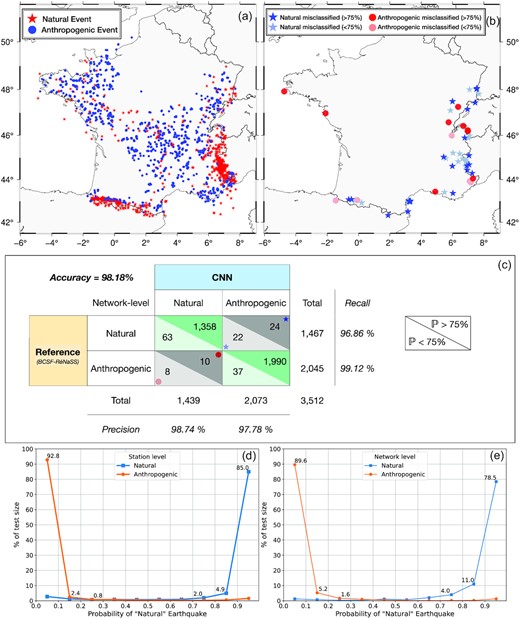
Application on the official French dataset detected between 2021 June 1 and November 1 from the BCSF-RéNaSS bulletin. (a) Geographic distribution of all seismic events used for this application (1450 natural and 2062 anthropogenic events). (b) Geographic distribution of events misclassified by the model. The blue stars correspond to events labelled as ‘natural’ and classified as ‘anthropogenic’ by the model. The red circles correspond to events labelled ‘anthropogenic’ and classified as ‘natural’ by the model. The darker colours correspond to a prediction of more than 75 per cent by the CNN and the lighter colours correspond to a prediction of less than 75 per cent by the CNN. (c) Confusion matrix, for the differentiation between natural and anthropogenic events, obtained from the French data set. The reference is the discrimination made by BCSF-ReNaSS. The classification is done at the network level. |$\mathbb {P}$| is the probability of an event. The symbols correspond to the events located on (b). (d) Normalized histogram of the output probability of being a natural earthquake for natural and anthropogenic earthquake detected between 2021 June 1 and November 1, at a station level and (e) at a network level.
Assuming that the discrimination made by national agency is reliable and can be used as reference, Figs 6(d) and (e) show probabilities obtained from the prediction for natural and anthropogenic events. Fig. 6(d) corresponds to the probabilities obtained at a station level, by taking into account each seismic trace independently. We observe that 95.2 per cent of the anthropogenic signals and 89.9 per cent of the natural signals are concentrated on the two edges of the probability range (between 0–0.25 and 0.75–1.0). At the network level (Fig. 6e), and taking into account all the stations for a given event, we observe that 94.8 per cent of the anthropogenic events and 89.5 per cent of the natural events are concentrated on the two edges of the probability range. This shows that the majority of the data are correctly classified with a high probability and confidence levels. In view of these results, we can establish a confidence level at 75 per cent probability to produce the confusion matrix.
Fig. 6(c) shows the results of the classification, at a network level, as a confusion matrix. The CNN model obtains high scores (accuracy of 98.18 per cent) with, in particular, recall for natural and anthropogenic events of 96.86 and 99.12 per cent, respectively. This indicates that, out of the entire database, approximately 3 per cent of the natural events and less than 1 per cent of the anthropogenic events are misclassified. Among the 1467 natural seismic events classified, 76 are located at less than 1 km depth. Our method thus correctly classified 70 of them (92.10 per cent). The precision indicates that 98.74 per cent of the predictions of natural events made by the model are correct. The F1 scores for natural and anthropogenic events are 97.79 and 98.46 per cent, respectively. This shows that the model is efficient in classifying natural and anthropogenic events on independent data. We can also observe that the majority of the predictions are made with a high level of probability: 3382 events (out of the 3512 in total) are classified by the model with a probability larger than 75 per cent.
Fig. 6(b) represents the location of the events misclassified by the CNN model. Among 3512 events, only 64 are not correctly classified by the model, which represents 1.82 per cent of the events. They seem to be located mostly on the eastern border of metropolitan France (zone B, Fig. 3).
3.2 University of Utah Seismograph Stations
The second application corresponds to events detected in the United States, Utah, in 2016. This data set offers the possibility to test the efficiency of our model in a drastically different context compared to the data used for its construction. The main idea is to check whether the CNN is able to discriminate anthropogenic events with characteristics (e.g. source function and power) that can differ from those in France.
Utah is seismically active due to its abundance of faults and fracture zones with, among the most active in Utah, the Wasatch Fault along the Wasatch Front (e.g. Arabasz et al. 1980). We use the event solutions including source location of events, labelled as natural or anthropogenic events, detected between 2016 January 01 and 2016 March 01 by University of Utah Seismographic Stations (UUSS). For each event, we recover seismic-waveform data only from three-component broad-band permanent seismometers located within 150 km of the earthquake location. P-wave times arrival were manually identified to extract the signals. This represents 1248 records of natural events (288 natural events) and 398 records of anthropogenic events (108 anthropogenic events). We use 49 permanent stations from UU (University of Utah 1962), WY (University of Utah 1983), NN (University of Nevada, Reno 1971) and AE (Arizona Geological Survey 2007) networks. The geographical distribution of all the events used for this application is represented in Fig. 7(a). The natural events are mainly located along active faults in the north–south direction with a clustering at Yellowstone in the north. The anthropogenic events are quarry blasts located on seven different quarries.
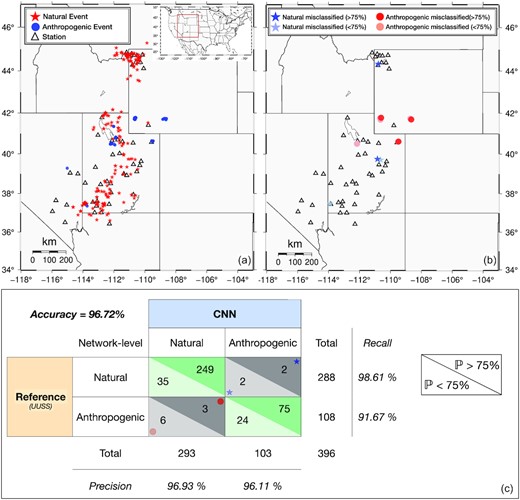
Application on events detected by UUSS between 2016 January 1 and March 1. (a) Geographic distribution of all the seismic events used for the application (288 natural and 108 anthropogenic events). (b) Geographic distribution of the events misclassified by the model. Blue stars correspond to the events labelled as ‘natural’ and classified as ‘anthropogenic’ by the model. Red circles correspond to the events labelled ‘anthropogenic’ and classified as ‘natural’ by the model. The darker colours correspond to a prediction of more than 75 per cent by the CNN and the lighter colours correspond to a prediction of less than 75 per cent by the CNN. (c) Confusion matrix, for the differentiation between natural and anthropogenic events. The classification is done at the network level. |$\mathbb {P}$| is the probability of an event. The symbols correspond to the events located on (b).
Assuming that the discrimination made by UUSS is reliable and can be used as reference, Fig. 7(c) shows the results of the classification at the network level. The CNN model again obtains high results with an accuracy of 96.72 per cent. The percentage is comparable to the results presented for the training phase. The natural and anthropogenic events obtain a recall of 98.61 and 91.67 per cent, respectively. This indicates that less than 2 per cent of the natural events and around 8 per cent of the anthropogenic events are misclassified. The F1 scores for the natural and anthropogenic events are 97.76 and 93.83 per cent, respectively. This scores is close to the end-2021 French data application. These very similar results indicate that the CNN seems to discriminate effectively between seismic events in two a priori different contexts.
Fig. 7(b) represents the geographic distribution of the events misclassified by the model. On the 396 seismic events, only 13 are not correctly classified. This represents 3.28 per cent of all the events. Moreover, we observe that 5 of the 9 misclassified anthropogenic events are located in areas where the nearest station is about 100 km away, which can explain this slightly higher percentage of misclassified anthropogenic events compared to the application on the French data.
3.3 Local post-seismic campaign
An earthquake of magnitude MW = 3.5 (Sira & Schlupp 2014) occurred near Vannes (NW France, see Fig. 8(a) for location) on 2013-11-21T09:53:00 (UTC). Six temporary stations were installed in a region of about 20 km around the main shock to document the aftershocks. Stations (three-component short-period velocimeters with a corner frequency of 1 Hz) were deployed for 26 d (between 2013 November 22 and December 17) and recorded ground displacement velocity with a sampling frequency of 100 sps. During this period, 48 events were detected, thanks to the STA/LTA approach (Haugmard 2016), close to the temporary station, including 36 natural events and 12 quarry blasts. This represents 173 records of naturals events and 66 records of anthropogenic events. The reference labels of these events were identified manually by observing the waveform, the location of the source, the origin time and the depth. Fig. 8(a) shows the location of the events detected during the post-seismic campaign. Although the data set is greatly reduced compared to the two other applications, we observe that the 12 quarry blasts originate from the same quarry and that 25 of the 36 natural events form a cluster that corresponds to the location of the main shock.
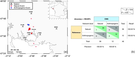
Application on temporary deployed seismic campaign installed near Vannes, in 2013, NW France. (a) Location of the natural (red stars) and anthropogenic events (blue circles) detected between 2013 November 22 and December 17. The triangles represent the temporary stations installed during the post-seismic campaign. (b) Confusion matrix, for the differentiation between the natural and anthropogenic events. The classification is done at the network level. The darker colours correspond to a prediction of more than 75 per cent by the CNN and the lighter colours correspond to a prediction of less than 75 per cent by the CNN.
Fig. 8(b) shows the results of the classification at a network level. The model obtained a remarkable score of 100 per cent meaning that all events detected during this post-seismic campaign, have been correctly classified by the model. The high performance of the classifier can be partly explained by the small epicentral distances where the source effect is more important than that of the propagation in the waveform.
4 DISCUSSION
4.1 Comparison with other methods
4.1.1 Features or not features?
The use of features extracted from the seismic signal is a widely used technique in machine learning. Renouard et al. (2021), for instance, use an hybrid approach including both human expertise and machine learning algorithms to achieve this objective. They trained a Random Forest algorithm by extracting selected features from the seismic signals and by implementing them in a decision tree. Their algorithm is trained with data recorded by permanent and temporary stations from the AlpArray Seismic Network (Hetényi et al. 2018) between 2016 and 2019 in the Upper Rhine graben area, in northwestern Europe. Their model achieve an accuracy of about 96 per cent. By applying our model only to the Upper Rhine graben area we obtain an accuracy of 97.8 per cent. Renouard et al. (2021) claim that their approach uses human expertise to compute features and thus avoids the ‘black box’ aspect of a classical neural network. However, the number of characteristics itself can be considered subjective and it is also possible that characteristics relevant for discrimination are omitted. Moreover, the use of algorithms such as Random Forest can lead to the use of many features that can be quite region specific and can thus limit the application of the algorithm to these specific areas. As a consequence, the workflow for such method can be quite complex. It is, for instance, required to first, pick the arrival times of the direct and refracted P and S phases, then, to locate the event and, finally, to extract from the signal the 22 features used by the algorithm to perform its prediction. The CNN, presented in this study, is only based on three component spectrograms that include a seismic event while achieving equivalent accuracy on a similar data set.
4.1.2 What does the spectrogram-based CNN bring?
The use of spectrograms to discriminate natural from anthropogenic events seems to give high classification performances. From Fig. 1, we can see that these spectrograms allow to highlight certain characteristic patterns of each of the two classes: (i) an energy that mainly impacts the low frequencies for the anthropogenic events (horizontal strips) and (ii) an energy that mainly impacts the whole frequency range for the natural events (vertical strips). The use of square filters (Table 1) makes it possible to analyse the image without preferential direction and to highlight these vertical and horizontal bands.
We can wonder whether the use of seismograms allows better performance than with spectrograms. We tried to train a CNN with seismograms using the same CNN architecture but with a 1-D version of the convolution layers. The input to the model corresponds to a matrix composed of three-components 60 s seismic traces. After ten training tests of this model the accuracy does not exceed 91.63 per cent. It would appear that the use of simple seismic traces does not capture spectral patterns and that the use of spectrograms allows for better performance. This statement seems to by confirmed by Liu et al. (2021) which also used a CNN to distinguish tectonic from non-tectonic earthquakes. By training their neural network with 100 s three-component waveforms provided by the China Earthquake Network Center (CENC), they achieve 92 per cent of accuracy.
4.1.3 Frequency range and time window width
Linville et al. (2019) also used a CNN to differentiate between natural and anthropogenic events. The architecture of their CNN is close to the one used in our study (Table 1) with four convolution layers with different number of filters and one fully connected layer. Their neural network is trained with UUSS data recorded between 2012 October and 2017 July. They use spectrograms computed on 90 s traces, between 1 and 20 Hz, producing matrices of size 40 × 48 × 3.
By training their CNN with a database of events detected in Utah, they achieve a recall of 99.1 per cent for natural events and of 99.3 per cent for anthropogenic events. These results are comparable but appear to be significantly better than those obtained with our approach. This may be due to the fact that to generate our model, we randomly select waveforms for the training, validation and test stages and not sets of traces associated with a given event. This subtlety necessarily leads to having traces of the same event in at least two of the three data sets used and then to apparently decreasing performances. When we apply our trained model to the UUSS data recorded from 2016 January to March, we obtain an accuracy of 96.72 per cent at the network level with a recall of 98.61 and 91.67 per cent for the natural and anthropogenic events, respectively. Taking into account only the events recorded by stations located at less than 100 km away, this accuracy rises to 97.95 per cent with a recall of 98.61 and 96.11 per cent for the natural and anthropogenic events, respectively. The difference in accuracy may be explained by several parameters like the size of the tested database, the training of the CNN on different geographical areas, the number of stations or the frequency range used for the classification. However, the use of spectrograms with a frequency content between 1 and 20 Hz limits the information usable by the CNN to extract features (such as vertical and horizontal stripes visible in Fig. 1), but also limits the seismic noise associated to human activities (traffic and industry).
Moreover, the window used to compute the spectrograms was selected using the P-wave time arrival. Thanks to these elements, the training can be simplified and the performance can be higher. The use of spectrograms with a frequency content greater than 20 Hz may be important for the differentiation of low magnitude earthquakes. Moreover, thanks to the data pre-processing, our model can recognize the nature of the event independently of its position in the spectrogram. Different tests were performed by positioning the arrival of the P-wave between 5 and 30 s after the beginning of the signal and the prediction results remain unchanged. Our approach can therefore be applied independently of the chosen detection method (STA/LTA, template matching, etc.) by randomly selecting the beginning of the windows studied.
4.2 Impact of the training database on predictions
4.2.1 Effect of variability in the training database
The approach described in this study discriminates with a large efficiency natural from anthropogenic seismic events. For this purpose, we trained a CNN with about 50 000 seismic signals recorded in metropolitan France. Our neural network is thus trained on a relatively small data set (compared to what can be found in the literature) though achieving high classification performances. To estimate the impact of the size of the database on the performance of the algorithm, we tested to train our CNN only with data coming from one of three distinct geographical areas in France (Fig. 3 and Table 2).
Data from Eastern France (zone B, Fig. 3) are balanced in terms of ratios between natural and anthropogenic events (namely 2612 natural events and 2415 anthropogenic events, Table 2) and represent half of the total database (22 818 records out of 50 000 total records). Training only with data from the zone B and applying this trained model on the events detected in Metropolitan France between 2021 June 1 and November 1, we obtain an accuracy of 98.14 per cent. The recall for the natural and anthropogenic events are 96.86 and 99.07 per cent, respectively. These results are very similar to those obtained when we train our CNN with the full database (with a recall for natural and anthropogenic events of 98.86 and 99.12 per cent, Fig. 6c), indicating that, even with a substantially reduced database, performance remains good.
In contrast, the zones A (nortwestern France) and C (Pyrenees) are unbalanced in terms of the proportion between natural and anthropogenic events (Table 2). Zone C contains more natural than anthropogenic events (namely 966 anthropogenic events and 2149 natural events). If we train the CNN with this database and apply it on the French data set, we obtain an accuracy of 97.5 per cent with a recall for the natural and anthropogenic events of 96.38 and 98.28 per cent. These results show that even with a lower proportion of anthropogenic events, performance remains high. We explain this by the fact that there is a sufficient variety (in terms of spectrogram patterns) of natural and anthropogenic events in the zone C to allow the CNN to be properly trained. On the other hand, the zone A presents significantly more anthropogenic than natural events (namely 255 natural events and 1407 anthropogenic events). By performing the same procedure as for the other zones, we obtain an accuracy of 89.83 per cent with a recall for the natural and anthropogenic events of 76.2 and 99.6 per cent, respectively. For this case, the classification performance collapses for the natural events. This can be explained by the fact that we probably do not have enough variety of natural event waveforms (Table 2) to achieve a robust classification. We performed a test to create a unbalanced database including events from the three zones. For this, 90 per cent of the events in the database are anthropogenic and 10 per cent are natural. By training our CNN with this database and applying the trained model on the French application data, we obtain similar results as when using only the zone A for training. It is therefore essential to have a large enough variety of natural events to obtain a good discrimination. However, the recall for the anthropogenic events remains excellent. This is likely due to the fact that, contrary to natural events, anthropogenic events have generally quite similar source functions and a limited range of magnitude (namely between 1.5 and 2.5). A more detailed interpretation would require a specific study and is beyond the scope of this work.
4.2.2 Effect of the training/validation-test ratio
An other drawback of the CNN training process is the selection of the proportion of the ‘training’ database (50,000 records in this study) that is used for the training, validation and testing phases. The results presented in Section 3 were obtained with a proportion of 80 per cent of the database for training and 20 per cent of the database for validation and testing. We present in Fig. 9 the performance of the algorithm using different training/validation-test ratios: 80/20 (original ratio), 60/40, 50/50, 40/60 and 20/80.
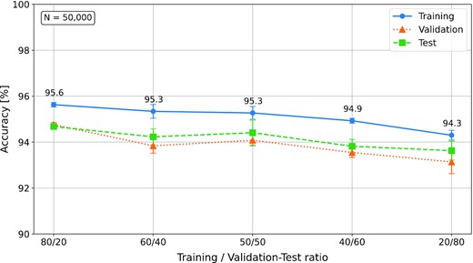
Performance of the CNN, at a station level, using different training/validation-test ratios. N corresponds to the total number of elements in the database. The accuracy obtained during the training, validation and test phases are represented in blue, orange and green, respectively.
Fig. 9 shows that our CNN reaches training accuracy of 95.6, 95.3, 95.3, 94.9 and 94.3 per cent for 80/20, 60/40, 50/50, 40/60 and 20/80 ratios, respectively. We thus observe a slight drop in accuracy with the decreasing in the amount of the initial database used for the trainig phase but, the performance remains high even when using only 20 per cent of the database (10 000 records). We also observe that the CNN achieves better performances (for validation and test) for a ratio of 50/50 compared to the 60/40 ratio. The origin of this observation is not clear and would require more investigation. It is clear from Fig. 9 that our initial choice of a 80/20 ratio seems to be optimal for training, validation and testing. We can conclude that the size of the training data set does not appear to be the primary factor that controls the discrimination performance whereas the diversity of signals in the database seems to be a key factor.
4.3 Impact of catalogue quality on predictions
4.3.1 Effect of seismic network geometry
The results presented in this study demonstrate the efficiency of the CNN for the classification of natural and anthropogenic events but also highlight that some events are misclassified by the neural network. Among other parameters, SNR of the data can be a factor impacting the performance of the model. A proxy to address this issue is the magnitude of the events, as the lower the energy the lower the SNR (for a given distance). Fig. 10(a) shows that, for Ml < 1 in the metropolitan France catalogue, about 3 per cent of the events are misclassified. Most of the events have 1 ≤ Ml ≤ 2 (68.00 per cent of the whole database) and, for these magnitudes, the accuracy reaches 98.45 per cent. Finally, for Ml > 2, the classes of all the 106 earthquakes are correctly predicted. Fig. 10(b), that shows the average SNR for each event, confirms that the discrimination is better in the highest SNR range. For SNR < 3, the accuracy collapses to 93.23 per cent while if the SNR is higher than 15, the accuracy reaches 99.01 per cent. Another parameter that impacts the performance of the model is the epicentral distance. Fig. 10(c) shows that the further the station is from the event, the lower the accuracy. For distances of more than 150 km, the accuracy drops to 92.63 per cent while for distances of less than 50 km, the accuracy reaches 97.02 per cent. This observation is also confirmed by the application on the data of the post-seismic campaign in NW France (Fig. 8). The average distance between the stations and the events is 16.89 km (Table S3, Supporting Information) and all these events were correctly classified by our method (Fig. 8b). We therefore believe that all of these parameters are in competition to obtain a classification.
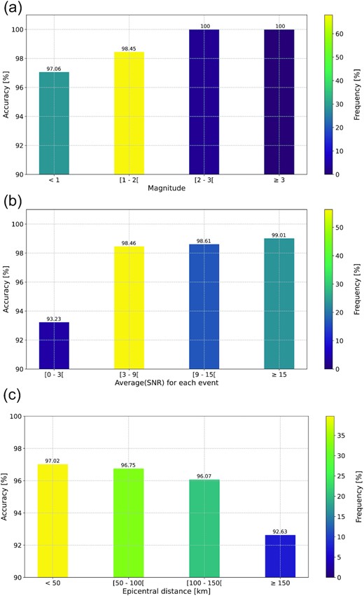
Discrimination performance as a function of magnitude, SNR and epicentral distance for events detected in metropolitan France between 2021 June 01 and November 01. (a) Relationship between CNN performance and event magnitude with accuracy marked at the top of the columns. The colour corresponds to the proportion of events for each magnitude range. (b) Relationship between the CNN performance and the average SNR of the events. The colour corresponds to the proportion of events for each SNR range. (C) Relationship between CNN performance and epicentral distance with accuracy marked at the top of the columns. The colour corresponds to the proportion of records for each distance range.
The lack of stations around an event also has an impact on the efficiency of the method. Fig. 7(b) that presents the geographical distribution of the misclassified events for the UUSS catalogue, shows that 5 of the 9 misclassified anthropogenic events are located at more than 100 km from the nearest station. Taking into account the events only recorded by at least one station within 100 km, the accuracy increases from 96.72 to 97.95 per cent. It can be noted, in Fig. 6(b) that most of the misclassified events are located at the borders of metropolitan France, and mainly in the zone C. Since we have only taken into account the stations of the FR network, for which distribution is limited to the French territory (Fig. 3), there is a lack of stations to the east of the French border. We performed a test on five natural events, located in the zone B, that were not correctly classified by the CNN. The stations network CH (Swiss Seismological Service (SED) 1983, located in Switzerland) and GU (University of Genoa 1967, located in Italy) were used to refine the prediction. These new stations are located within 50 km from the events, whereas the stations used in the FR network are more than 60 km away. The addition of these stations for the classification allows to correctly classify these five events. This indicates that the epicentral distance is an important parameter affecting discrimination as shown in Fig. 10(c). In addition, increasing the number of stations aroung event can improve the variability of waveforms induced by their radiation pattern.
4.3.2 Effect of the mislabebled events in the database
Finally, a misclassified event can also be simply due to mislabelled events in the database. During the manual inspection of the data for the generation of the confusion matrices we were indeed able to identify some mislabelled events in the database. In Fig. 11(a), we present the trace and spectrogram of an event detected on 2019-08-02T20:09:00 UTC labelled as a ‘quarry blast’ and that was classified as a ‘natural event’ at 99.4 per cent by the CNN. This event is undoubtedly a natural event because no quarry blast occurs at such a late hour (10 p.m. local time). In addition, the spectral characteristics of natural event presented in Section 2.1 are clearly observe here (Fig. 11a) two seismic wave arrivals that form a vertical band in the spectrogram. In contrast, Fig. 11(b) shows a signal from a seismic event that occurred on 2021-08-03T09:50:00 UTC. This event is tagged as ‘natural’ in the database but classified at 99.9 per cent as ‘anthropogenic’ by our trained model. The spectrogram of this event is characterized by the impulsive arrival of the P wave and by two horizontal strips along the time axis at frequency between 1 and 30 Hz. Thanks to the time of origin of the event (11:50 a.m., local time) and to the characteristics of the seismic signal, we can reasonnably consider that this event is correcly classified as ‘anthropogenic’ by the CNN. Those examples illustrate the importance of having trusted database for training but shows that a well-trained CNN can help to detect, a posteriori, inconsistencies in the databases and would allow the reassessment of the associated labels.
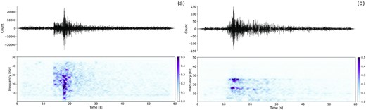
(a) Spectrogram of an earthquake, detected on 2019 August 2 at 22:09, local time, recorded by the VIEF station, at a distance of 25.16 km from the source, labelled ‘anthropogenic’ and classified by the CNN at 99.4 per cent as ‘natural’. (b) Spectrogram of an earthquake, detected on 2021 August 3 at 11:50 a.m., local time, recorded by the LOUF station, at a distance of 65.52 km from the source, labelled ‘natural’ and classified by the CNN at 99.9 per cent as ‘anthropogenic’.
5 CONCLUSION
The objective of this study is to develop a method for automatic discrimination of natural and anthropogenic events in order to reduce the data processing time. Based on recent existing methods, we have developed a CNN to perform this discrimination using spectrograms. We have constituted a training database composed of BCSF-RéNaSS events detected in metropolitan France. By adapting the pre-processing of the data, our CNN is able to recognize the nature of the event independently of the position of the earthquake in the signal and thus to discriminate the events directly after the detection phase. This trained model achieves high classification performance with, for example, an accuracy of 98.18 per cent when applied to independent French data. By applying the model on data from different geographical areas and geological contexts, we show the versatility of our approach. For the UUSS application, the model achieved an accuracy of 96.72 per cent. These applications to other geographical areas have shown the robustness of the model in recognizing characteristic patterns in different databases. We observed a certain redundancy of features present in the spectrograms involving a continuous energy in time and discontinuous in frequency for anthropogenic events, represented by a horizontal linearity on the spectrograms. Inversely, for natural events, we observe a discontinuous energy in time and continuous in frequency, represented by a vertical linearity on the spectrograms. These features highlight the relevance of using square filters (Table 1) in the CNN, to not focus on one direction in the spectrogram.
This approach can be used as an aid to discriminate, in real time, the detected seismic signals. We can propose an application with human interaction, where the analyst can check only the events with lower probabilities, for example, less than 75 per cent. Moreover, we could highlight mislabelled events present, for example, in the BCSF-RéNaSS bulletin. These mislabelled events can be reclassified by the CNN and thus allow to constitute a catalogue as reliable as possible.
SUPPORTING INFORMATION
Figure S1: Examples of four natural events (A, B, D and F) and four anthropogenic events (C, E, G and H), recorded by the FR network stations, with the associated spectrograms. The seismic signals correspond to the normalized raw data of the vertical component. The spectrograms are normalized by their maximum. All technical details of the events are in Table S2.
Table S1: Useful information about the records shown in Fig. 1, where: d is the source-station distance, z is the depth of the event, SNR the signal to noise radio and MLv the local magnitude on the vertical component. The acronyms eq and qb stand for natural event (earthquake) and quarry blast respectively.
Table S2: Useful information about the records shown in Fig. S1, where: d is the source-station distance, z is the depth of the event, SNR the signal to noise radio and MLv the local magnitude on the vertical component. The acronyms eq, qb and exp stand for natural event (earthquake), quarry blast and explosion respectively.
Table S3: Statistical informations of the three databases used in the application (Section 3). Standard deviations are denoted σ. No magnitude is available for Vannes dataset.
Please note: Oxford University Press is not responsible for the content or functionality of any supporting materials supplied by the authors. Any queries (other than missing material) should be directed to the corresponding author for the paper.
ACKNOWLEDGEMENTS
The authors warmly thank the anonymous reviewers for their constructive criticism and to the editor for their work. This work was only made possible by the manual discrimination performed by BCSF-RéNaSS operators (R. Dretzen, S. Lambotte and M. Grunberg, http://renass.unistra.fr).
Résif-Epos is a Research Infrastructure (RI) managed by the INSU,CNRS. It is a consortium of 18 French research organizations and institutions, included in the roadmap of the Ministry of Higher Education, Research and Innovation. Résif-Epos RI is also supported by the Ministry of Ecological Transition.
DATA AVAILABILITY
This work included data from the permanent seismic networks operated by the French seismological and geodetic network (RESIF), by UUSS and temporary stations from a post-seismic campaign deployment near the city of Vannes in 2013. Catalogues and data from the French National Observing Service (BCSF-RéNaSS) and the UUSS are available using an International Federation of Digital Seismograph Networks (FDSN) protocol.
The discrimination code is available on Git (doi:10.5281/zenodo.7064191). The algorithms are written with Python and data processing is based on Python libraries Obspy (Krischer et al. 2015), Scipy (Virtanen et al. 2020) and Numpy (Harris et al. 2020). We use Tensorflow (Abadi et al. 2015) for implementations and iterate model parameters using Keras (Chollet 2015). Our figures were generated using Matplotlib (Hunter 2007) and The Generic Mapping Tools (GMT, Wessel et al. 2019).
REFERENCES
,
