


SUMMARY
The proliferation of large seismic arrays have opened many new avenues of geophysical research; however, most techniques still fundamentally treat regional and global scale seismic networks as a collection of individual time-series rather than as a single unified data product. Wavefield reconstruction allows us to turn a collection of individual records into a single structured form that treats the seismic wavefield as a coherent 3-D or 4-D entity. We propose a split processing scheme based on a wavelet transform in time and pre-conditioned curvelet-based compressive sensing in space to create a sparse representation of the continuous seismic wavefield with smooth second-order derivatives. Using this representation, we illustrate several applications, including surface wave gradiometry, Helmholtz–Hodge decomposition of the wavefield into irrotational and solenoidal components, and compression and denoising of seismic records.
1 INTRODUCTION
The character of progress in observational seismology has to a large extent been controlled by the quality and quantity of data. As such, the increasing availability of seismic arrays with large numbers of instruments (large-N arrays) to the research community has become one of the major instrumentation themes of 21st century seismology. Array seismology brings both opportunities, in the form of spatial analysis techniques such as backprojection (Kiser & Ishii 2017), eikonal/Helmholtz tomography (Lin et al. 2009; Lin & Ritzwoller 2011) and wave gradiometry (Langston 2007a,b; de Ridder & Biondi 2015), as well as challenges associated with processing ever larger data volumes (Kennett & Fichtner 2020). These technical trends will increase as more large-N array data is recorded, especially with the advent of Distributed Acoustic Sensing (DAS) arrays, from which data sets with many thousands of channels recorded at 100 Hz are now routinely recorded (e.g. Lindsey et al. 2017; Li & Zhan 2018; Williams et al. 2019; Yu et al. 2019).
One of the most significant opportunities presented by large-N arrays is the transition from collections of individual seismograms to unified analysis of the seismic wavefield as a single entity, for which we can evaluate the ground motion at an arbitrary point in time and space within the array. In this study we use the term wavefield reconstruction to describe the process of synthesizing individual seismograms into a coherent product. This product allows for additional analyses, such as robust wavefield gradiometry (de Ridder & Biondi 2015), which fully utilize the behaviour of the wavefield in both space and time.
Ensuring that seismic instruments are of sufficiently high quality to measure ground motions to high fidelity in time was one of the great instrumentation achievements of the last century of seismology. However in most research settings, spatial sampling of the wavefield is insufficiently dense to capture all details of interest within the desired temporal frequency bandwidth. Because seismic arrays used in research settings typically only take sparse and uneven spatial measurements, the development of methods for optimal reconstruction of the continuous wavefield is an open research question. Industry scale results have typically focused attention to the problem of optimally filling missing or corrupted channels in an otherwise regularly sampled deployment. Much effort in industry has recently focused on time and scale localized transforms (e.g. Herrmann & Hennenfent 2008; Herrmann et al. 2008), which can allow for sparser representation of complex wavefields and consequently improved robustness of the reconstruction under noise, but for which the most efficient algorithms require structured data volumes.
At regional scales, methodologies have had to contend with the aforementioned spatial sparsity. Suggested methods have included perturbations of a reference plane wave by smoothed splines (Sheldrake 2002), applicability of which is limited to single phases with constant slownesses across the array; radon transforms using a general plane wave basis (Wilson & Guitton 2007); compressive sensing (CS) using a plane wave basis (Zhan et al. 2018); and recently tensor completion methods utilizing local rank reduction to capture curved wave fronts (Chen et al. 2019). Past regional scale wavefield reconstruction methods have focused primarily on plane wave based reconstructions due to their attractive theoretical properties and potential for good angular resolution given adequate array design; however, the plane wave assumption performs poorly for wavefields close to the source or with local scattering, for which the full spatial frequency spectrum is required to reconstruct the wavefield, leading to difficulties in resolving the required plane wave coefficients.
In this study, we present a wavefield reconstruction method based on wavelet analysis, specifically employing temporal wavelet analysis on individual seismic channels and then employing weighted curvelets for spatial analysis. This algorithm allows for a fully time/space and scale localized transform on unstructured seismic data. The underlying physics of wave propagation in continuous media is controlled by balancing the rate of change of momentum in a volume with the stress gradients (and body forces) applied to the volume through Newton’s second law: |$\rho \ddot{u_i} = \sigma _{ij,j} + f_i$|. If the constitutive relationship of the medium is elastic, the stresses σij are expressed in terms of strains σij = cijklϵkl with |$\epsilon _{kl} = \frac{1}{2}(u_{i,j} + u_{j,i})$| (Aki & Richards 2002). These fundamental relationships of wave physics suggest an important consideration in wavefield reconstruction; namely, that the physical wavefield does not depend on the displacement field itself, but rather its second time derivative, and, approximately, its’ second spatial derivatives. This implies that any wavefield reconstruction algorithm must attempt to not only fit the data, but also produce physically reasonable second derivatives if wave physics is to be respected. Accurately recording the spatial derivatives of the wavefield places significantly tighter constraints on the quality and density of the recorded wavefield than does merely recording the undifferentiated ground motions. The wavefield reconstruction algorithm presented in this study promotes the reconstruction of wavefields that obey wave physics by introducing a Laplacian based pre-conditioner into the compressive-sensing optimization problem, and by recognizing that due to the non-stationary power content of earthquake wavefields, a time-frequency representation is required to optimize the regularization of the spatial reconstruction transform. After introducing the algorithm, we present three case studies utilizing real seismic data to emphasize practical applications.
2 WAVEFIELD RECONSTRUCTION ALGORITHM
2.1 Data quality control and processing
For the purposes of designing a data quality control and processing workflow, the most notable characteristic of the proposed wavefield reconstruction algorithm is that the final, compressive-sensing, step it is performed on the whole data volume of an array simultaneously, rather than on a trace-by-trace basis. Therefore, the algorithm requires that each individual trace has an equivalent instrument response, or, if a heterogeneous collection of instruments is being used, that the instrument response is removed from all traces to obtain true ground motions. Because the regularized curvelet inversion utilized in the spatial reconstruction step uses a least-squares metric for assessing data fit, it is relatively sensitive to amplitude outliers. Consequently, all examples in this paper using real data sets were manually checked for malfunctioning channels, which were removed. For larger data sets, it is likely that an automated procedure for identifying malfunctioning channels is required, however as the method is likely to change depending on application, we have not presented a general strategy here and instead describe what actions have been taken for each example individually.
2.2 Wavelet transform
After initial processing of the data, each record is then transformed into a time–frequency representation via a wavelet transform. The wavelet transform comes in both continuous and discrete forms—heuristically both act by representing the signal in terms of a scalings and translations of an underlying mother wavelet. The behaviour with scale encodes the frequency characteristics of the signal, while the translations encode behaviour in time. The choice of using a discrete (DWT) or continuous (CWT) wavelet transform is determined by the objective of the study.
The CWT has the advantage that it permits explicit processing in the time-frequency domain, for example wavelet based denoising and windowing as suggested by Mousavi & Langston (2016) and Langston & Mousavi (2019). However, the CWT is redundant and so the computational complexity and storage requirements of employing it are high. Fig. 1 shows two filtered seismic waveforms and the amplitude of their time–frequency representations by employing the CWT using a Morlet mother wavelet. The most salient feature of the time-frequency representations of the CWT is that the signal power depends strongly on time within the signal for each frequency, and strongly on frequency at each time; that is the signal is non-stationary within the time-frequency domain. This suggests that the optimal regularization parameter for CS in the curvelet domain is likely to be different for each wavelet coefficient.
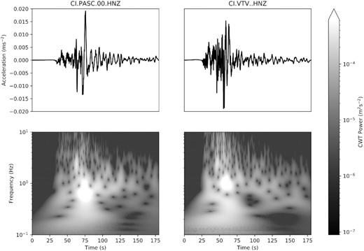
Continuous wavelet transform (CWT) of two strong ground motion accelerograms of the 2019 July 6 Mw 7.1 Ridgecrest earthquake. The CWT highlights the general observation that the power of signals from seismic events is typically non-stationary in both time and frequency.
The DWT provides a more computationally efficient transform than the CWT. The implementation details of DWT transforms are substantially more involved than that of the CWT—we refer the reader to Starck et al. (2010) for a review. In contrast to the CWT, the DWT is not redundant, however the choice of mother wavelet for DWT analysis is non-trivial and typically requires some a priori knowledge or test data to optimize the DWT representation, as the final reconstruction performance can be significantly impaired by a bad choice of mother wavelet, compared to the generally robust CWT for seismic data using Morelets (Mousavi & Langston 2016; Langston & Mousavi 2019). Additionally, the structure of the DWT means that it is not suitable for time-frequency analysis; however, it often forms a suitable representation for data compression and denoising. For reasons of computational efficiency, all of the case studies that follow employ the DWT for time-frequency analysis; however, CWT based redundant reconstructions based on the Morelet typically produce the best results and may be necessary if the highest quality is required. We have found that the Daubechies wavelet family typically performs well for the examples shown in this study.
2.3 Compressive sensing in the curvelet domain
A frame that is particularly suited to use in seismic applications is the curvelet frame, which has been designed to promote sparsity for signals with wave-propagation like properties (Candes & Demanet 2005). The k-space support of an individual curvelet is a dartboard-like wedge segment, which gives curvelets directional sensitivity, as well as scale localization (Candès et al. 2006). Curvelets are constructed to obey a parabolic scaling relationship with the spatial extent perpendicular to wave propagation scaling like the square root of that parallel to propagation, which accounts for their directional sensitivity—see Fig. 2. The curvelet frame has consequently been used in industry scale reconstruction and denoising applications using CS (e.g. Herrmann et al. 2008; Herrmann & Hennenfent 2008; Hennenfent & Herrmann 2006; Hennenfent et al. 2010), for synthetic regional scale examples applied to surface wave tomography (Zhan et al. 2018) and recently as a filter for scattered waves by Zhang & Langston (2019), who employed the explicit curvelet transform for densely sampled data interpolated to a regular grid rather than the optimization based approach employed here for sparse data.
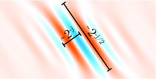
Example curvelet in the spatial domain showing angular sensitivity and characteristic parabolic scaling relationships between wavef-ront-parallel and wave-front perpendicular directions.
An optimal interpolation at points sampled by another sampling matrix |$\mathbf {\hat{\Psi }}$| is given by |$\mathbf {\hat{\Psi } \Phi P \hat{m}}$|. This formulation differs slightly from the normal presentation in that we have included an additional weighting matrix |$\mathbf {P}$|, that rescales the basis coefficients to reflect desired properties. In particular, curvelets are indexed by a scale jc (as well as rotation and translation indices). To promote smoothness of the second derivative, we employ |$\mathbf {P} = Diag(2^{{-j_c}^n})$| as our weighting matrix, which penalizes rapid oscillation of the reconstructed signal. Application of this matrix is in effect somewhat similar to applying Tikhonov regularization to the CS problem, with n = 2 corresponding to smoothing by penalizing the Laplacian of the wavefield, however it removes the need for a second regularization parameter and also puts the problem in a form that can be used by all existing L1 solvers.
2.4 Reconstruction
Reconstruction of the wavefield, either for recorded seismic channels, or at unobserved synthetic channels, is performed by generating the matrix |$\mathbf {\hat{G}}$| with rows |$\mathbf {\hat{G}}_k$| that describes the sampling-basis transform-weighting product |$\mathbf {\Psi \Phi P m}$| evaluated at the channels indexed by k. The predicted wavelet coefficients for each channel are then given by |$\hat{w}_k(j_w,s) = \mathbf {\hat{G}}_k\mathbf {\hat{c}}(j_w,s)$|. The time domain signal for the channel is then recovered by performing an inverse wavelet transform |$\hat{u}_k(t) = IWT(\hat{w}_k(j_w,s))$|. For the CWT, the inverse transform is not unique due to the redundancy of the transform and an appropriately normalized inversion wavelet must be prescribed to take this into account; in contrast the DWT has a unique inverse transform (Daubechies 1992). It must be noted that this synthesis step encodes the regularizing assumptions inherent in the previous analysis steps that allow us to write the wavefield as a collection of curvelet coefficients in space and wavelet coefficients in time, namely that coherently propagating waves are present in the wavefield and we expect them to have smooth Laplacians. As such, any further usage of the wavefield must be consistent with these assumptions.
2.5 Summary
To summarize the methods detailed above, we propose the following generic algorithm for wavelet–curvelet wavefield reconstruction:
Individual traces ui(t), indexed by channel i and time t, are quality controlled to ensure timing and amplitude are correct.
Individual traces ui(t) are put into a time–frequency representation using a common wavelet transform to give a collection of wavelet coefficients wi(jw, s) = WT(ui(t)) indexed by time shift s, channel i and wavelet scale jw.
For each wavelet coefficient, an L1 regularized optimization problem of the form given in eq. (6) is solved to determine sparse curvelet coefficients |$\mathbf {\hat{c}}(j_w,s)$| for shift s and wavelet scale jw describing the spatial distribution of the wavelet coefficients wi(jw, s) across the array.
To evaluate the ground motion at a particular location indexed by k, we form the curvelet reconstruction matrix |$\mathbf {\hat{G}}_k$|, and the reconstructed ground motion is given by |$\hat{u}_k(t) = IWT(\mathbf {\hat{G}}_k \mathbf {\hat{c}}(j_w,s))$|
3 WAVEFIELD GRADIOMETRY FOR THE SOUTHERN CALIFORNIA ARRAY
Array based seismic wavefield tomography techniques, in particular eikonal tomography (Lin et al. 2009), have, in the last decade, become a major component of the regional–global structural seismic workflow, especially in the context of ambient-noise cross-correlation data sets (e.g. Lin et al. 2014; Bowden et al. 2017; Berg et al. 2018, 2020). These methods use various combinations of derivatives of wavefield observables to obtain information such as surface wave phase velocities. Because of the difficulty of accurately computing derivatives on a sparse collection of data and the resultant amplification of noise, this class of techniques is a good target for wavefield reconstruction as a first step in data processing so as to obtain robust derivatives.
As an example of this, we performed a wave equation gradiometry tomography experiment for the Southern California Seismic Network (SCSN). Wave equation based gradiometry, in particular, places the highest quality requirements on the Laplacian of the wavefield as it utilizes the phase of the wavefield, in addition to its amplitude. Obtaining reasonable values of phase velocity from wave equation gradiometry therefore serves as a practical demonstration that the wavefield reconstruction is accurately recovering the true wavefield, up to the second derivatives in space and time.
The interquartile range of the distances to the four nearest neighbour stations in the SCSN, calculated across the network, is 14–28 km. This corresponds to a station spacing of between 2.5 and 5 stations per wavelength for a period of 20 s, assuming a nominal phase velocity of 3.5 km s−1, and up to 7–14 stations/wavelength for 50 s period waves with, assuming a nominal phase velocity of 4 km s−1. As such, large parts of the SCSN fail to match the 10 stations/wavelength requirement for wavefield gradiometry in this period band, which is a typical band for earthquake based array tomography methods.
For the source wavefield, we utilized the Rayleigh wave packet of the 2017 November 19 Mw 7.0 Loyalty Islands earthquake (GCMT code 201711192243A; Dziewonski et al. 1981; Ekström et al. 2012). This earthquake had a shallow normal faulting mechanism that directed strong Rayleigh waves towards California. We analysed the BHZ channel of the SCSN, integrated to displacement and filtered between 10 and 100 s. Quality control was performed on a per-trace basis by calculating the maximum normalized cross-correlations between a test trace and the signal at all other stations, and then requiring that at least 50 per cent of these normalized cross-correlation values be better than 0.6 for the test trace to be retained. Additionally, we required that the root-mean-square log amplitude be within three standard deviations of the average across stations. These quality control measures resulted in a final array of 221 stations from an initial set of 234 with data. The wavefield reconstruction was performed using a 64 × 128 pixel curvelet transform, with the db4 wavelet (the Daubechies family wavelet with four vanishing moments) used for the temporal transform. Fig. 3 shows a cross-section of the reconstruction results for this earthquake. After performing the reconstruction, we apply narrow band Butterworth filters with a width of |$1/\sqrt{20}$| the period, and then calculate Cp using eq. (7). Examples of this are also shown in Fig. 3, and show that the scaled Laplacian does typically fit the acceleration records well for this data. The resulting phase velocity curves are physically reasonable, and match the theoretical phase velocity curves from the CVM-H model (Shaw et al. 2015) well, especially within the basin. Fig. 4 shows a spatial map of the phase velocity recovered for a period of 45 s. The wave equation gradiometry discussed here does not formally account for finite frequency effects as we do not constrain the wavefield to fit the wave equation; to handle this, and reduce the variance of the results, we apply radial basis function smoothing using a multiquadratic basis function with length scale 45 km (approximately 1/4 wavelength), and only report results for points within the convex hull of stations within 90 km of that point. The equivalent model without radial basis function smoothing is shown in Supporting Information Fig. S2. These results are comparable to existing surface wave tomography maps in the same period band (Lin & Ritzwoller 2011), but are derived directly from a single earthquake, giving us good confidence that the reconstruction algorithm is accurately capturing the details of the wavefield.
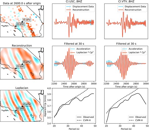
Wavefield gradiometry for the Southern California Seismic Network applied to the Rayleigh wave packet of the 2017 November 19 Mw 7.0 Loyalty Islands earthquake. We show the BHZ channel integrated to displacement and its reconstruction for one basin station (USC) and one high desert station (VTV), filtered between 10 and 100 s. We also show a comparison between the measured accelerations at 30 s and the spatial Laplacian multiplied by a single coefficient, interpreted to be the squared phase velocity at the channel site—showing that the Rayleigh wave packet closely follows the acoustic wave equation at this period. Finally, we show the estimated phase velocity curves and their comparisons to the theoretical phase velocities derived from the CVM-H model—the agreement between the observed data and the theoretical model is quite good and has been achieved from a single wave packet from a single earthquake.
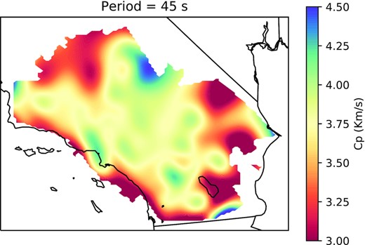
Phase velocity map of Southern California at a period of 45 s for points within the convex hull of nearby SCSN stations (<90 km distance), recovered using Laplacian based wavefield gradiometry of a single event, the 2017 November 19 Mw 7.0 Loyalty Islands earthquake. The tomographic model is smoothed using a multiquadratic radial basis function with a length scale of 45 km to suppress artefacts at length scales shorter than 1/4 of the characteristic wavelength.
4 HELMHOLTZ–HODGE DECOMPOSITION OF THE HORIZONTAL WAVEFIELD
As an example of utilizing wavelet–curvelet CS for performing the Helmholtz–Hodge decomposition, we visualize the wavefield from the Mw 7.1 July 6 2019 Ridgecrest Earthquake, recorded at the LAUSD-CSN. The LAUSD-CSN is a low-cost, high-density permanent urban seismic deployment utilizing micro-electromechanical system (MEMS) accelerometers, straddling the Northeastern edge of the Los Angeles basin (Clayton et al. 2012; Kohler et al. 2020). The network is optimized for cheap, spatially resolved near real-time strong-ground motion reporting from earthquakes within the Los Angeles metro area and consequently uses instruments with a high instrument noise floor. However, the ground motions from the regional Mw 7.1 Ridgecrest event were sufficiently strong to produce waveforms that are a near match to the acceleration seismograms of colocated permanent strong-ground motion instruments (HN channel, example comparison for station CI.PASC in Supporting Information Fig. S1). The location of the LAUSD-CSN relative to downtown Los Angeles, and the curvelet inversion domain utilized in the Helmholtz–Hodge decomposition are shown in Fig. 5(a).
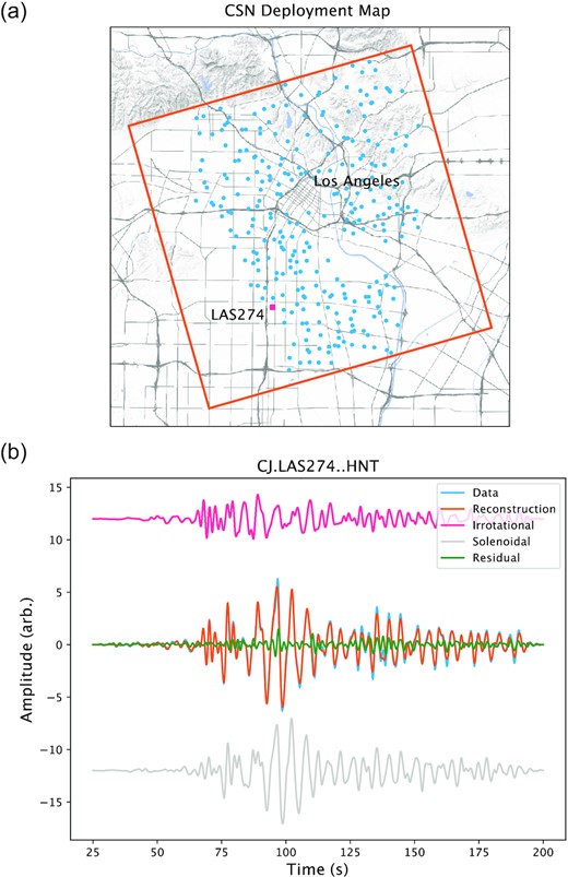
(a) Los Angeles Unified School District–Community Seismic Network (LAUSD-CSN) accelerometers used in this study are shown in blue, with station LAS274 shown by a pink square. The inversion domain is shown by the orange square. The Los Angeles downtown is the high density area of roads in the centre of the figure. (b) Data, reconstruction and residual for the tangential component of the Ridgecrest 2019 July 5 Mw 7.1 Earthquake recorded at LAUSD-CSN station CJ.LAS274. The irrotational and solenoidal components are individually shown offset from the main waveform and show the strong solenoidal Love wave arriving after the SV/SH arrival observed on both components. Waveform is bandpass filtered between 0.5 and 15 s.
The inversion utilized acceleration waveforms bandpass filtered between 2 and 15 s, a 64 × 64 pixel spatial curvelet transform, and the db12 wavelet for the time domain transform. The CS optimization problem was solved with Elastic-Net regression with α = 0.95. The LAUSD-CSN team discovered that a number of sensors were misoriented during the Ridgecrest event; these sensor problems have confirmed by site visit and corrected. Additional potentially misoriented sensors have been detected by analysing apparent spatial discontinuities in long-period particle motion. In that case, rotations in 90° increments have been manually applied to bring the long-period motions into alignment—in these cases the misorientation is likely a result of placement of the instrument against the incorrect wall of an interior room. An example time-domain reconstruction is shown in Fig. 5(b), showing the ability of the Helmholtz–Hodge decomposition to extract the large Love-wave component into the solenoidal term. A still frame from the resulting Helmholtz–Hodge decomposition, 75 s after the event origin time, is shown in Fig. 6—the full video is available online in Supporting Information. The frame shown in Fig. 6 is during the surface wave packet. The contributions of the Rayleigh and Love waves can be seen in the irrotational and solenoidal components of the field, respectively. The irrotational component in particular shows the strong bending of Rayleigh waves as they cross into the deep Los Angeles basin from the northeast
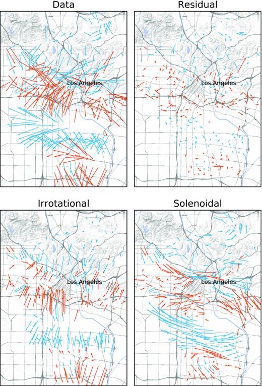
Helmholtz–Hodge decomposition of the horizontal wavefield of the Mw 7.1 2019 July 6 Ridgecrest event recorded on the LAUSD-CSN network. The wavefield is plotted 75 s after the event origin time. Arrows show the horizontal particle instantaneous acceleration for both data and reconstruction. Arrows are coloured with the sign of the real data vertical component to highlight the oscillatory structure of the wavefield.
5 WAVEFIELD COMPRESSION
A final, simple, application of the wavefield reconstruction technique detailed here is as a lossy data compression algorithm. While the wavefield reconstruction algorithm proposed here is not optimized for data compression, the use of a sparsity promoting domain transform naturally induces compression when the wavefield is sufficiently coherent. In general seismic data (especially in research settings) is able to be stored as high fidelity continuous time-series, however there are at least two significant end-member cases for which compression techniques are potentially applicable. The first is in extremely dense industry-scale surveys, in which the total data volume becomes prohibitively difficult to handle. The tension between periods of high data acquisition and continually advancing computational storage and processing capabilities, has lead to cycles of interest in seismic data compression as a means to reduce the computational burden (e.g. Villasenor et al. 1996; Herrmann et al. 2008; Da Silva et al. 2019). The majority of these studies have focused on structured seismic data volumes, potentially with some missing elements, and so have achieved high compression ratios while maintaining fidelity—a peculiarity of the current study is that our algorithm is targeted at unstructured data volumes, necessitating the mixed-type wavelet–curvelet decomposition described above. The second end-member is that of slow data transmission-rate scenarios, such as those that will be encountered by proposed planetary seismology arrays (e.g. Marsal et al. 2002; Neal et al. 2019; Zhan & Wu 2019). This scenario motivated initial studies into seismic data compression, such as that of Wood (1974), where the rate of data acquisition outpaced that of early telephone based remote communication protocols. In this scenario, onsite pre-processing before transmission may allow more detailed (either more channels or higher sampling frequency) data to be transmitted than would otherwise be the case. We briefly discuss the ability of the algorithm proposed in this study to compress the wavefield within the context of a local strong-ground motion accelerometer array (CSN).
For CSN data set resampled at 2 Hz and filtered using a zero-phase bandpass filter between 2 and 50 s, applying the proposed wavelet–curvelet reconstruction method using a db4 wavelet for DWT achieves a compression ratio of 8.3. The recovery of the original signal can be quantified by the a scaled mean-squared-error fidelity metric |$1 - \sqrt{\frac{1}{N_s}\sum _{j=1}^{N_s}\frac{1}{N_d}\sum _{i=1}^{N_d} (\mathbf {d}_{ij}-\mathbf {\hat{d}}_{ij})^2/Var(\mathbf {d})}$|, which gives a value of 0.71 using the for the CSN data set. The residuals from the above case studies are largely incoherent with the recorded wavefield, suggesting that the reconstruction is acting as a denoising filter (noting that “noise” in this context includes scattered energy that is not able to be sparsely represented using the curvelet frame). We do not attempt to optimize the transform parameters for compression, and it is likely that further investigation would yield improved compression ratios for equivalent fidelity. In particular, for the purposes of compression, it may not be necessary to accurately obtain accurate spatial derivatives, so changing the form of the pre-conditioning matrix may promote sparser transforms.
In our scheme, compression occurs entirely during the sparsity promoting Elastic Net regularized curvelet inversion—all wavelet coefficients are inverted for. It is possible that higher compression ratios for equivalent reconstruction accuracy could be obtained by further sparsifying the temporal component in the wavelet domain. Temporal sparsification would, however, have to be designed to be consistent with the spatial patterns of the waveforms, which may be difficult due to the propagation of the wavefield. As such, further studies into compression schemes based on the joint wavelet–curvelet transform are left for future research.
6 DISCUSSION AND CONCLUSIONS
The three real-data examples shown in this work illustrate the required modifications to the framework presented in Zhan et al. (2018) to robustly handle sparse, noisy, realistic wavefield recordings. We have developed the theory in this paper for point sensor recordings, however with minor modifications it can equally be employed for DAS or mixed DAS and point sensor deployments. Because the algorithm presented here relies on timescale (wavelet) or position-angle-scale (curvelet) transforms, there is significant scope for tailoring the algorithm toward specific data sets, that we have not fully explored. In particular, in the time domain, we have found that the Daubechies family typically works well, but that is not to say that other wavelet families may not be equally or even more performant. In the spatial domain, curvelets are well suited for seismic applications (Herrmann & Hennenfent 2008; Herrmann et al. 2008), but other transforms such as wave atoms may work well (Leinonen et al. 2013). For large apeture deployments such as the USArray, where the Earth’s curvature becomes important, employing natively spherical transforms such as spherical curvelets (Chan et al. 2017) may be necessary. Future work to address, in particular, the best combination of both transforms to promote sparsity of the spatial transform and hence good CS performance will improve the accuracy of the reconstruction. Given this flexibility, the key intellectual contribution of this paper is then to propose independent reconstructions in time and space to handle the sparse, unstructured data sets present in research deployments, and to recognize the importance of appropriately reweighting the spatial reconstruction frame to promote continuity of higher order derivatives, if the wave equation is to be satisfied.
Looking forward to future methodology for wavefield reconstructions of unstructured seismic data sets, recent machine learning (ML) applications of physics-informed neural networks (PINNs) (Raissi et al. 2019) promise to allow for grid-free reproduction of seismic wavefields (Karimpouli & Tahmasebi 2020; Moseley et al. 2020; Song et al. 2020). Current research has focused on training for wavefield solvers based on known synthetic velocity models, however there is potential for the same computational structure to be used in a joint inversion of unknown velocity structure with observed data, under reasonable assumptions that some seismic wave equation is satisfied; given observational constraints the first likely route would be for surface wave reconstruction / phase velocity inversion as is presented in this study. PINN based studies originating from within the geophysics community have utilized computational architectures originally proposed for general discovery of PDE behaviour—that is they have not been specifically optimized for seismic applications. In particular, these studies have made use of non-periodic activation functions, which fail to exploit the inherent quasi-periodicity of the seismic wavefield. Recent work on neural networks utilizing periodic activation functions (Sitzmann et al. 2020) and / or analysis in the Fourier domain (Li et al. 2020) may therefore improve the potential of ML based methods for wavefield reconstruction. In particular, the work of Sitzmann et al. (2020), utilizing sinusoidal activation functions in a network they term SIRENS, has proven to be able to very accurately reconstruct the higher order derivatives of seismic wavefields necessary for computing terms in the seismic wave equation. This is due to the property that the derivative of a SIREN is also a SIREN, which allows for analytical computation of non-vanishing second-order derivatives with inherent periodicity. Thus far, the training of PINNs has proven to be relatively computationally expensive and work has been largely limited to synthetic examples, however the field is still in its nascent stage and currently appears to hold great promise for the large class of PDE constrained inverse problems, in which wavefield reconstruction may be included.
We have presented a general strategy for wavefield reconstruction of unstructured seismic data using wavelet / curvelet transforms, as well as specific implementation details for three example applications. This framework allows for the conversion of point seismic time-series into a single unified data product, suitable for spatial analyses of the seismic wavefield such as wavefield gradiometry, backprojection, reverse-time migration, etc. Our choice of the curvelet basis for spatial analysis allows for the recovery of complex wavefields including multipathing or backscattering effects. Our framework promotes a physically concordant wavefield by appropriately penalizing short wavelength fluctuations without requiring a priori knowledge of the underlying velocity structure or requiring iterative solutions of the wavefield reconstruction problem. It therefore represents a simple and flexible way to compress and represent the seismic wavefield, suitable for irregularly sampled networks at all scales.
SUPPORTING INFORMATION
Figure S1. Comparison between Southern California Seismic Network strong ground motion station CI.PASC.00.HN* and Community Seismic Network station CJ.T000337.HN* for the Mw7.1 2019 July 5 Ridgecrest earthquake. These stations are approximately colocated. The waveforms have been decimated to 5 Hz, detrended and lowpass filtered at 1 Hz. Amplitudes have been scaled to approximately account for instrument gain.
Figure S2. Rayleigh fundamental mode phase velocities derived from wavefield gradiometry for Southern California using the 2017 November 19 Mw 7.0 Loyalty Islands earthquake. This version uses simple 2-D linear interpolation as opposed to radial basis function smoothing, as shown in Fig. 4.
Please note: Oxford University Press is not responsible for the content or functionality of any supporting materials supplied by the authors. Any queries (other than missing material) should be directed to the corresponding author for the paper.
ACKNOWLEDGEMENTS
The authors would like to thank the editor, Andrew Valentine, and an anonymous reviewer, for their insightful reviews that clarified several points. They would also like to thank Charles Langston for a particularly enthusiastic review. JBM acknowledges the financial support of the Origin Energy Foundation and the General Sir John Monash Foundation during his PhD studies. ZZ thanks the support from NSF CAREER award EAR 1848166 and the NSF/IUCRC GMG Center. Seismic data were processed using Obspy (Beyreuther et al. 2010), and figures were created using Matplotlib (Hunter 2007) using Cartopy for mapping (Met Office 2010).
DATA AVAILABILITY
Data for the Mw 7.0 Loyalty Islands Earthquake were obtained through the obspy FDSN service using the Southern California Earthquake Data Center as a provider (SCEDC 2013). CSN data for the Mw 7.1 Ridgecrest Earthquake are available through the CSN website at http://csn.caltech.edu/data/. Code and data to recreate the Helmholtz–Hodge decomposition are available at https://github.com/jbmuir/HelmholtzHodgeCSN.
