


SUMMARY
Late-time transient electromagnetic (TEM) data contain deep subsurface information and are important for resolving deeper electrical structures. However, due to their relatively small signal amplitudes, TEM responses later in time are often dominated by ambient noises. Therefore, noise removal is critical to the application of TEM data in imaging electrical structures at depth. De-noising techniques for TEM data have been developed rapidly in recent years. Although strong efforts have been made to improving the quality of the TEM responses, it is still a challenge to effectively extract the signals due to unpredictable and irregular noises. In this study, we develop a new type of neural network architecture by combining the long short-term memory (LSTM) network with the autoencoder structure to suppress noise in TEM signals. The resulting LSTM-autoencoders yield excellent performance on synthetic data sets including horizontal components of the electric field and vertical component of the magnetic field generated by different sources such as dipole, loop and grounded line sources. The relative errors between the de-noised data sets and the corresponding noise-free transients are below 1% for most of the sampling points. Notable improvement in the resistivity structure inversion result is achieved using the TEM data de-noised by the LSTM-autoencoder in comparison with several widely-used neural networks, especially for later-arriving signals that are important for constraining deeper structures. We demonstrate the effectiveness and general applicability of the LSTM-autoencoder by de-noising experiments using synthetic 1-D and 3-D TEM signals as well as field data sets. The field data from a fixed loop survey using multiple receivers are greatly improved after de-noising by the LSTM-autoencoder, resulting in more consistent inversion models with significantly increased exploration depth. The LSTM-autoencoder is capable of enhancing the quality of the TEM signals at later times, which enables us to better resolve deeper electrical structures.
1 INTRODUCTION
Transient electromagnetic (TEM) method is a powerful technique in several geophysical exploration applications such as mineral exploration, groundwater monitoring, geological hazard mitigation and oil reservoir imaging (Zhdanov & Portniaguine 1997; Auken et al. 2003; Newman & Commer 2005; Haber et al. 2007; Yang & Oldenburg 2012; Qiu et al. 2013; Li & Huang 2014; Yogeshwar et al. 2019). TEM techniques use a grounded wire or an ungrounded loop as a source to transmit a step-off current that induces a time-varying electric field (Nabighian & Macnae 1987) containing electrical information about the subsurface resistivity structure.
However, TEM responses decay exponentially with time, imposing a major limitation on the depth of penetration. Responses arriving earlier in time are characterized by large-amplitude high-frequency components with strong attenuation and small diffusion depths, whereas later responses correspond to small-amplitude low-frequency contents with weak attenuation and deeper penetration (Nabighian & Macnae 1987). In particular, the late-arriving responses are often superimposed by ambient noises arising from both natural sources with, for example, sferics caused by thunderstorms or geomagnetic field micro-pulsations, and man-made structures such as power grids, communication cables or buried pipelines (Munkholm & Auken 1996).
Without sufficient noise suppression, late-arriving low-amplitude inductive information cannot be extracted from TEM data to explore deep underground structure. Therefore, effective and efficient methods are required to obtain improved signals. Such schemes allow us to make full use of the information from deeper underground to interpret the TEM data, and ensure the success of field experiments. Numerous efforts have been made on removing noise from TEM data in both time and frequency domains, using for example principal component analysis, wavelet transform and noise estimation methods (Kass & Li 2011; Ji et al. 2016; Rasmussen et al. 2017). They either rely on repeated observations with high experimental costs or focus on high-frequency components only. In general, the noise sources and characteristics are complex and unpredictable. Moreover, TEM responses and noises often overlap in both time and frequency domains. Therefore, TEM data often contain residual noises even after going through the existing de-noising procedures.
To recover the TEM responses more effectively and accurately, we employ a specific architecture of deep learning methods named LSTM-autoencoder, which is achieved by using a particular kind of recurrent neural network (RNN) known as the long short-term memory (LSTM) network (Hochreiter & Schmidhuber 1997; Gers et al. 2000) based on an autoencoder architecture (Rumelhart et al. 1986; Vincent et al. 2008, 2010).
With the rapid development of computer technology, deep learning has been successfully applied recently in various fields such as speech recognition (Deng et al. 2013), intelligent translation (Cheng et al. 2016) and image processing (Litjens et al. 2017). In particular, these methods have been proved to be powerful in learning feature representations and adaptable to different tasks and data sets. Instead of focusing on the detailed physical processes, models based on machine learning extract the complex and implicit relationships between the input and output data sets, with the effectiveness dependent on the completeness of the training data set.
When it comes to geophysics, deep learning algorithms are mostly utilized for automatic picking of seismic arrival times (Dai & MacBeth 1995; Zhu & Beroza 2018; Dokht et al. 2019), seismic lithology prediction (Zhang et al. 2018), seismic inversion (Röth & Tarantola 1994), and electrical resistivity inversions (Spichak & Popova 2000; van der Baan & Jutten 2000). Due to its remarkable effectiveness, the LSTM network has stood out in time-series applications such as speech recognition and natural language processing (Sak et al. 2014; Palangi et al. 2016). Meanwhile, autoencoder is mainly used in data compression and feature extraction with symmetrical topological structures (Le et al. 2013), which is well-suited for de-noising tasks (Vincent et al. 2008, 2010). Combining the LSTM network with autoencoder structure has proven to be effective in extracting data features and analysing time-series in automatic acoustic detection (Marchi et al. 2015), solar power forecasting (Gensler et al. 2016) and human movement prediction (Ghosh et al. 2017). In particular, the LSTM-autoencoder achieves an outstanding performance on automatic speech recognition containing additive noise (Coto-Jiménez et al. 2016). The current study is the first application of the LSTM-autoencoder to TEM de-noising, providing a powerful support for subsequent data applications.
2 THE LSTM-AUTOENCODER
In this section, we briefly review the deep learning architectures used for the de-noising procedure and introduce the LSTM-autoencoder architecture for TEM data de-noising.
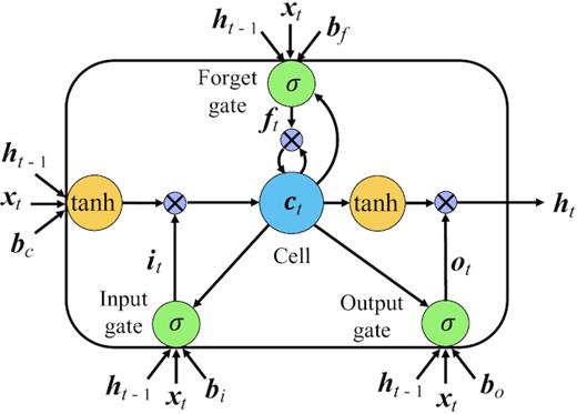
A long short-term memory block containing a memory cell and the input, output and forget gates (modified from Gers et al. 2000).
Vincent et al. (2008, 2010) proposed the stacked de-noising autoencoder to recover the clean data from distorted inputs by assuming that features obtained by the autoencoder should be more robust if the network pays more attention to the overall distribution of data rather than the minute details such as noise or small disturbances.
The de-noising algorithm aims to minimize the loss function by adjusting the parameters in the weighting matrix |${\boldsymbol{W}}$| and the bias |${\boldsymbol{b}}$| in eq. (9). As a consequence, the whole de-noising procedure is transformed to a least-squares problem, which can be solved by any gradient-based optimization method. Due to the complex structure of the network, it is difficult to calculate the partial derivatives for the huge set of parameters. However, the backpropagation algorithm can be used to obtain the partial derivatives of the loss function, which allows us to complete the neural network training and minimize the loss function in eq. (9) iteratively by the gradient descent method.
3 SYNTHETIC EXPERIMENTS
3.1 Synthetic data sets
Since it takes a significant amount of time and effort as well as funding to collect sufficient field TEM data with natural noise, and ideal noise-free data are unavailable, here we train the LSTM-autoencoder on synthetic data sets generated by 1-D forward modelling with and without noises added. Fig. 2 illustrates the setting of the unified transmitter–receiver device with a transmitter loop as a source and 24 receivers to record |${{{\rm{d}}{B_z}}}/{{{\rm{d}}t}}$|, the time derivatives of the vertical-component magnetic fields. A total of 1000 1-D resistivity models, that is, layered structures extending infinitely in horizontal directions, are created with resistivity |$\rho $| in the range of |$1\!-\!1000{\rm{\ \Omega }}\cdot{\rm{m}}$|. In all models, the number of layers is randomly set between 1 and 20 with the bottom depth at |$1000{\rm{\ m}}$|. Fig. 3 shows three examples of the models. A total of 24 000 |${{{\rm{d}}{B_z}}}/{{{\rm{d}}t}}$| transients are calculated at 24 receiver locations as the target values of the network output. Noise is then added to all the transients to obtain input data for the LSTM-autoencoder. The entire data set with 24 000 |${{{\rm{d}}{B_z}}}/{{{\rm{d}}t}}$| transients is randomly divided into training and test sets with a ratio of 7:3, that is, 16 800 for the training set and 7200 for the test set. The training set is used to tune the parameters in the network, while the test set does not participate in the training but only probes whether the network overfits the samples in the training set. Every transient is sampled at a uniform interval on a logarithmic timescale with 1000 sampling points covering the time range of |${10^{ - 5}}\!-\!1{\rm{\ s}}$|.
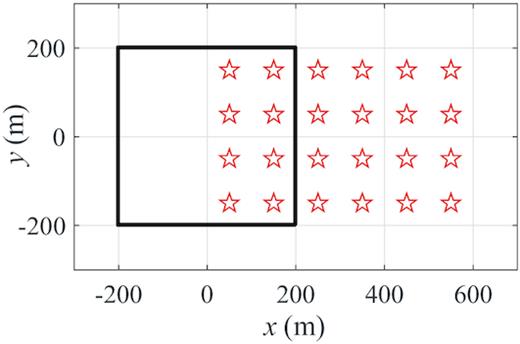
Configuration of the transmitter–receiver device used in generating synthetic data set. Transmitter loop source and receivers are shown by the thick black line and red stars, respectively.
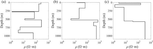
Three examples of the 1000 1-D resistivity models used in generating the synthetic data sets.
During the training process, the inputs of the network are the noise-added TEM soundings |${{{\rm{d}}{B_z}}}/{{{\rm{d}}t}}$|, while the outputs are the de-noised TEM responses for the corresponding inputs. The similarity between the actual and estimated noise will greatly affect the adaptability and effectiveness of the LSTM-autoencoder to newly acquired signals. To demonstrate the broader applicability of the LSTM-autoencoder, we used four types of common noises in the forward modelling responses. Note that we cannot cover all realistic field conditions with respect to the spatial-temporal dependence of noise.
The first type is the Gaussian noise with a constant variance determined by the amplitudes of the signals in each time-series, which corresponds to environmental noise with stable fluctuations (Figs 4a and b); the second one is also Gaussian noise but with different amplitudes at different sampling points, representing systematic errors caused by the receiver instruments (Figs 4c and d); the third one involves random impulsive signals to simulate the sferics caused by thunderstorms (Figs 4e and f); while the fourth type of the noise simulates the industrial power disturbance with a sinusoidal oscillation at a specific frequency of 50 Hz mixed with a random interference (Figs 4g and h). For the inputs of the network, each TEM transient is added with a mixture of all four kinds of noise. Fig. 5(a) shows the superposition of all four types of noises shown in Fig. 4, while Fig. 5(b) displays the noise-free transient as well as the transient with noise superimposed. The transient in the latter case cannot be used without de-noising since the noises already overwhelm the signals at early to intermediate times.
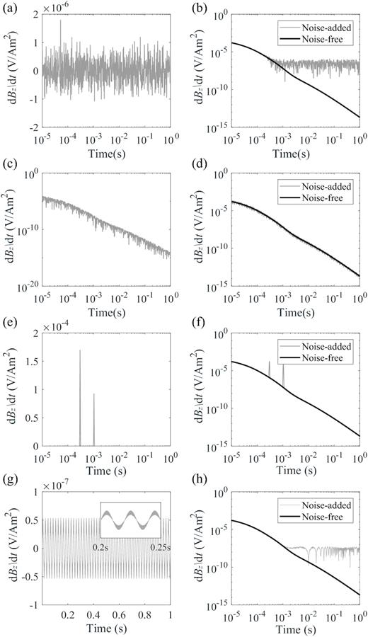
Four types of noises and examples of noise-free and noise-added TEM responses. (a) Gaussian noise with a constant variance for all sampling points. (b) An example of the noise-free and noise-added TEM responses. (c and d) Same as (a) and (b) but for Gaussian noise with different amplitudes for different sampling points. (e and f) Same as (a) and (b) but for random impulsive noises. (g and h) Same as (a) and (b) but for a noise of a 50 Hz sinusoidal oscillation mixed with a random interference.
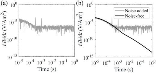
(a) A mixture of the four types of noises shown in Fig. 4. (b) TEM responses with and without the noise in (a).
Here we have used extremely long simulated TEM transients which decay to about |${10^{ - 14}}\ {\rm{V}}\,{\rm{A}}^{-1}\,{{\rm{m}}^{-2}}$| later in time and cannot be detected by the equipment. If the LSTM-autoencoder can restore the characteristics of later signals with a noise level of |${10^{ - 7}}\ {\rm{V}}\,{\rm{A}}^{-1}\,{{\rm{m}}^{-2}}$|, it will certainly be effective for shorter transients with a higher signal-to-noise ratio (SNR).
3.2 Error measurements
3.3 Implementation details
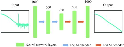
The LSTM-autoencoder architecture. The input is the noise-added TEM transients with 1000 sampling points evenly spaced on a logarithmic timescale. The output is the corresponding de-noised TEM data. The green stripes represent layers inside the neural network, with the number on top denoting the layer dimension. The blue and orange arrows are the LSTM encoders and decoders, respectively, applied between layers.
The RMSPE values of the training and test sets are monitored throughout the training process. After 300 epochs, the RMSPE value of the test set rises slightly while that of the training set no longer decreases significantly with the increase of epoch number, which indicates that the LSTM-autoencoder has converged to the minimum level of the loss function without overfitting at around 300th epoch. As Fig. 7 shows, the RMSPEs of the training and test sets approach to the small values of 0.35% and 0.98%, respectively, when the training epoch number reaches 300.
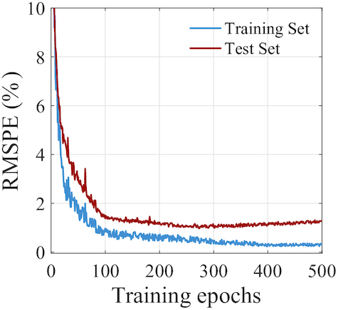
Decreases in the error measurement RMSPEs of the training (blue) and test (red) sets with training epochs.
The network tuned at the 300th epoch is selected as the final well-trained de-noising network. It has acquired the implicit features of signal and noise by finding an optimal combination of the weighting matrix W and bias vector b. The de-noising performance of the LSTM-autoencoder on the test set consisting of 7200 transients without participating in the network training is thoroughly inspected and none of the results are misinterpreted. A sample pair is randomly selected and the comparison between the de-noised and noise-free signals is shown in Fig. 8, where the relative errors of the LSTM-autoencoder de-noise result (red line in Fig. 8b) are less than 1% for most of the sampling points. Although the input noise-added signal is severely perturbed by the noise after ∼2 ms (Fig. 8a), the output from the LSTM-autoencoder matches the noise-free signal almost perfectly for all times. Furthermore, the relative errors of the entire test data sets are evaluated, and the average values are close to zero with standard deviations less than 0.01 (Fig. 8b), indicating a stable de-noising effect.
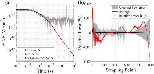
(a) An example of the outputs from the LSTM-autoencoder and its comparison with noise-added and noise-free signals. (b) Relative errors of the whole test sets and the transient in (a). The red solid line shows the relative errors between the output and noise-free signals for all sampling points in (a). The black line is the average relative errors at individual sampling points of the whole test data set with standard deviation shown in grey shading.
4 DISCUSSION
4.1 Comparison with conventional de-noising methods
The most widely-used technique to suppress random noise in TEM is stacking (e.g. Yogeshwar et al. 2019) and filtering techniques for harmonic noise. In addition, wavelet transform and principle component analysis (PCA) have also been proposed to improve the SNR of TEM data (Kass & Li 2011; Ji et al. 2016). Fig. 9 shows the de-noising performance under different noise conditions by means of stacking, wavelet threshold method, PCA and LSTM-autoencoder. The usual approach of stacking is to calculate the mean of a given stack, which is efficient for rejecting incoherent or stationary noises in a statistical sense, such as Gaussian noise, or noise whose mean values are close to zero, such as a 50-Hz power noise. However, stacking cannot deal effectively with impulsive noises occurring only occasionally to a single sample in time and requires long recording times with mass data storage. Frequency-based wavelet threshold method performs better in removing noises with special frequency characteristics, but fails to suppress sharp impulsive noises and causes distortions in samples early in time when the noise and signal spectra overlap with each other. PCA can only reduce part of the noises, but not remove them completely. In Fig. 9, we use both individual and the combination of three types of commonly occurring noises in TEM data to assess the effectiveness of the different de-noising techniques. Obviously different de-noising techniques are developed to tackle different types of noises, and Fig. 9 clearly illustrates that the conventional de-noising techniques may perform well for one or two types of noises, but none of them can simultaneously suppress all three types of noises on its own. In contrast, the well-designed LSTM-autoencoder is capable of handling all these types of noises satisfactorily, without requirement for spectrum analysis or other identification processes for noise characteristics.
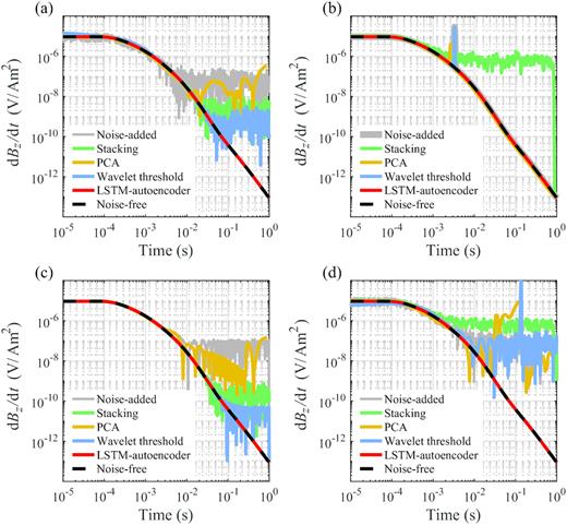
(a) Comparison of de-noised results by stacking (green), PCA (yellow), wavelet threshold method (blue) and LSTM-autoencoder (red) with a mixture of the two Gaussian noises in Figs 4(a) and (c). (b) Same as (a) but for an impulsive noise. (c) Same as (a) but for a 50 Hz sinusoidal noise. (d) Same as (a) but for a mixture of the four types of noises in (a)–(c).
4.2 Comparison with several well-known networks
To verify the effectiveness of our proposed network for noise removal, we conduct quantitative comparisons with several other well-known deep learning algorithms including the autoencoder, the fully connected (FC) and the LSTM networks. Table 1 shows the final |${\rm{RMSPE}}$| values of the test set using these completely trained networks. The large RMSPE values result from the deviation in the order of magnitude between the de-noised data and noise-added signal at later times. Among the four networks, the LSTM-autoencoder achieves the lowest value of RMSPE, which demonstrates that it has the best performance in late-time signal recovery. An example of the outputs from the four networks for the same noise-free and noise-added TEM signals and their relative errors are presented in Fig. 10, which shows clearly that the LSTM-autoencoder performs the best among the four networks. Meanwhile, the |${\rm{SNRs}}$| defined in Section 3.2 are listed in Table 2. It can be seen that among the four networks the LSTM-autoencoder yields the largest |${\rm{SNR}}$| value. The late-arriving signals, which carry information from relatively deep medium and are often overwhelmed by noises, are always challenging in de-noising efforts. Table 2 also presents the |${\rm{SNR}}$| comparison for the results after 2 ms when the signal is severely distorted by noise, which demonstrates significant improvement in |${\rm{SNR}}$| achieved by the LSTM-autoencoder. These numerical results confirm that the LSTM-autoencoder yields de-noised TEM data that are in best agreement with the noise-free signals.
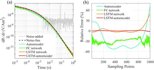
An example of the LSTM-autoencoder de-noise result and comparison with three other commonly used networks. (a) Noise-free and noise-added signals plotted together with the de-noise results by different networks. (b) Relative errors between the de-noise results by different networks and the noise-free signal for all sampling points.
Comparison of the |${\rm{RMSPE}}$| values of the test data set for the four types of networks.
| Data sets | Autoencoder | FC network | LSTM network | LSTM-autoencoder |
|---|---|---|---|---|
| |${{\rm RMSPE}}\ ( \% )\ $| | |$34.42$| | |$29.56$| | |$9.36$| | |$0.98$| |
| Data sets | Autoencoder | FC network | LSTM network | LSTM-autoencoder |
|---|---|---|---|---|
| |${{\rm RMSPE}}\ ( \% )\ $| | |$34.42$| | |$29.56$| | |$9.36$| | |$0.98$| |
Comparison of the |${\rm{SNR}}$| values of the entire de-noised signals and de-noised signals after 2 ms from the four types of networks for the example shown in Fig. 10.
| |${\rm{SNR}}$| (dB) | Noise-added | Autoencoder | FC network | LSTM network | LSTM-autoencoder |
|---|---|---|---|---|---|
| Entire signal | 10.08 | 12.28 | 9.89 | 22.70 | 27.18 |
| Signal after 2 ms | −16.38 | 5.93 | 10.86 | 23.77 | 30.82 |
| |${\rm{SNR}}$| (dB) | Noise-added | Autoencoder | FC network | LSTM network | LSTM-autoencoder |
|---|---|---|---|---|---|
| Entire signal | 10.08 | 12.28 | 9.89 | 22.70 | 27.18 |
| Signal after 2 ms | −16.38 | 5.93 | 10.86 | 23.77 | 30.82 |
4.3 Application of the de-noised signals in 1-D resistivity inversions
The enhanced capability for noise removal by the LSTM-autoencoder has important implications in many geophysical applications. Here, we illustrate this by comparing 1-D resistivity inversion results based on de-noised data sets from the four well-trained networks with that using the original noise-free signal. Fig. 11 shows the configuration of the transmitter–receiver device and the 1-D resistivity model used to generate the synthetic data set |${{{\rm{d}}{B_z}}}/{{{\rm{d}}t}}$|. The noise-free and noise-added data sets at receiver R (Fig. 11a) are shown in Fig. 11(b) together with the transients from different de-noising networks. We use the inversion technique of Li et al. (2016) to derive 1-D resistivity models from the different data sets. The results are compared with the original 1-D model in Fig. 11(c). The noise-added transient is completely dominated by the noise from ∼1 ms (Fig. 11b), which causes large discrepancy between the inversion result and the original model at depths below ∼250 m. Table 3 lists the RMSPEs of the inversion results using noise-added and de-noised data sets in comparison to the result obtained from the noise-free data. Among all de-noising networks, the LSTM-autoencoder clearly achieves the best result with the smallest discrepancy, yielding a model closest to that obtained from the noise-free data set. We define the sensitivity as the percentage change of |${{{\rm{d}}{B_z}}}/{{{\rm{d}}t}}$| caused by a unit resistivity perturbation to the current model. Fig. 11(d) shows the sensitivities of all sampling points in the TEM signal recorded at receiver R to the resistivities at different depths. Sensitivities to shallower structures are mainly provided by earlier signals of |${{{\rm{d}}{B_z}}}/{{{\rm{d}}t}}$|, whereas later ones are more sensitive to the structures at greater depths. After ∼0.15 s, |${{{\rm{d}}{B_z}}}/{{{\rm{d}}t}}$| is clearly dominated by the resistivity at greater depths, as shown by the orange curve for the 1200-m depth in Fig. 11(d). The sensitivity curves demonstrate that if noise is successfully removed from TEM data after ∼0.15 s such that the weak signals can be extracted effectively, the resolvable depth of resistivity can be extended significantly. Theoretically, we can probe the subsurface down to ∼1200-m depth assuming the model and de-noised transient in Fig. 11. However, the exploration depth and detectability of a deep target depend heavily on the data errors at later times.
![(a) Configuration of the transmitter–receiver device used in 1-D resistivity inversion test. The transmitter loop source and receivers are shown by the thick black box and red stars, respectively. (b) Noise-free and noise-added signals at receiver R in (a) propagated in the synthetic 1-D model [black-solid in (c)] plotted together with the de-noise results by the autoencoder (light blue), the FC (green), LSTM (orange) and LSTM-autoencoder (red) networks. (c) Comparisons between the original 1-D resistivity model (black solid line) with inversion results using data sets in (b). (d) Sensitivity values of ${{{\rm{d}}{B_z}}}/{{{\rm{d}}t}}$ collected from receiver R to the resistivities of several underground depths: 100, 325 and 1200 m. The sensitivity values to the depth of 1200 m are significantly larger after ∼0.15 s.](https://oup.silverchair-cdn.com/oup/backfile/Content_public/Journal/gji/224/1/10.1093_gji_ggaa424/1/m_ggaa424fig11.jpeg?Expires=1749844091&Signature=rkvlub~uZfmNaJ1ldBG~4XMOJsDvJ3RPEfjUR3h3oKUP~jKAsQj6Xm5rPS7SHLclshKs3jNxBeLmiFGLFA5wTz7YS-E0tdC8AQ~6hV7sI5L9UMoBAIJs8R3IH6PAXOjmCb-nXfDUuK6A3D4~FGcTPVoiEJNxH6Ho4OyoA1e8KZi1AdtRbbtfRoEVvZv-C0n5EY5bm8HnktvsdIyFZYAhG3TL9nnmhEFZCtbHke0deF2MGB9H-Kp2svU~H1CI4suhUeRkHDkyHtG5iRUMejj-L7HCccbGqMaDrRT5Mnm5v4h1V8tGt~UQgVVXGUmIOdQI7Y2n80unlR0CcGTLmISZVw__&Key-Pair-Id=APKAIE5G5CRDK6RD3PGA)
(a) Configuration of the transmitter–receiver device used in 1-D resistivity inversion test. The transmitter loop source and receivers are shown by the thick black box and red stars, respectively. (b) Noise-free and noise-added signals at receiver R in (a) propagated in the synthetic 1-D model [black-solid in (c)] plotted together with the de-noise results by the autoencoder (light blue), the FC (green), LSTM (orange) and LSTM-autoencoder (red) networks. (c) Comparisons between the original 1-D resistivity model (black solid line) with inversion results using data sets in (b). (d) Sensitivity values of |${{{\rm{d}}{B_z}}}/{{{\rm{d}}t}}$| collected from receiver R to the resistivities of several underground depths: 100, 325 and 1200 m. The sensitivity values to the depth of 1200 m are significantly larger after ∼0.15 s.
The |${\rm{RMSPEs}}$| of inversion results using noise-added and de-noised data sets by the four networks relative to inversion result using noise-free data.
| Data set | Noise-added | Autoencoder | FC network | LSTM network | LSTM-autoencoder |
|---|---|---|---|---|---|
| |${{\rm RMSPE}}\ ( \% )\ $| | |$57.55$| | |$25.50$| | |$41.59$| | |$12.21$| | |$3.46$| |
| Data set | Noise-added | Autoencoder | FC network | LSTM network | LSTM-autoencoder |
|---|---|---|---|---|---|
| |${{\rm RMSPE}}\ ( \% )\ $| | |$57.55$| | |$25.50$| | |$41.59$| | |$12.21$| | |$3.46$| |
4.4 De-noising of 3-D TEM signals
To further demonstrate the general applicability of the LSTM-autoencoder, we conduct a de-noising experiment using a 3-D model with a typical TEM loop source set-up, as shown in Fig. 12. The 3-D resistivity structure consists of a low-resistivity cube buried in the top layer of a five-layer model. The low-resistivity cube has a resistivity value of 20 |${\rm{\ \Omega }}\cdot{\rm{m}}$| and is buried below the centre of the transmitter loop, with its top at 146-m depth and a dimension of 190 m × 190 m × 177 m. Two arbitrary receiver locations are selected, with one inside the transmitter loop and the other outside. We add three different noise-levels to the transients: mild, medium and heavy with amplitudes of |${10^{ - 8}}$|, |${10^{ - 7}}$| and |${10^{ - 6}}{\rm{\ V}}\,{\rm{A}^{-1}}\,{{\rm{m}}^{-2}}$|, respectively. The de-noising results show that for different levels of added noise, the LSTM-autoencoder achieves significant SNR enhancement, as shown in Table 4. The signal after ∼1 ms is completely dominated by noise and is most challenging in the de-noising task. The LSTM-autoencoder effectively removes the noise with an increase of SNRs by about 80 dB. This experiment clearly shows that the LSTM-autoencoder provides an excellent de-noising capability with significant enhancements in SNR to TEM signals generated by 3-D structures with different noise levels.
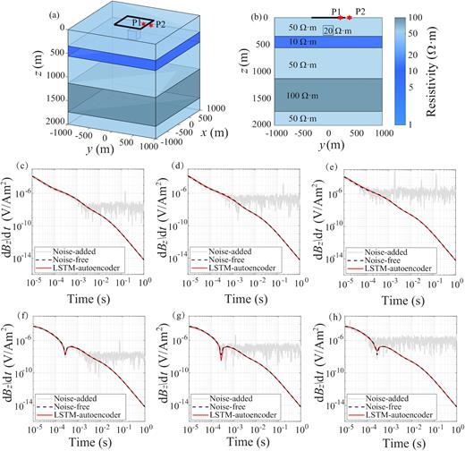
(a) A 3-D resistivity structure with a transmitter–receiver device on the surface. The black box depicts the transmitter loop source with 600 m on each side. Two arbitrary receiver locations are selected on the surface, with one inside the transmitter loop (P1, y = 220 m) and another outside (P2, y = 389 m). (b) A vertical cross-section at x = 0. (c) Comparison of noise-free (grey) and noise-added (black) signals at P1 with de-noised result. (d) Same as (c) but with medium noises. (e) Same as (c) but with heavy noises. (f) Same as (c) but for signals at P2 with mild noises. (g) Same as (f) but with medium noises. (h) Same as (f) but with heavy noises. In (c)–(h), the black and grey lines are noise-free and noise-added TEM responses, while the red curves are the de-noised results from the LSTM-autoencoder.
SNR enhancement for 3-D TEM signals with different noise levels.
| |${\rm{SNR\ }}( {{\rm{dB}}} )$| of entire signal | |${\rm{SNR\ }}( {{\rm{dB}}} )$| of signal after 1 ms | ||||
|---|---|---|---|---|---|
| Receiver | Noise level | Before de-noising | After de-noising | Before de-noising | After de-noising |
| P1 | Mild | 12.46 | 38.65 | −11.29 | 35.21 |
| Medium | 11.37 | 20.56 | −29.23 | 23.55 | |
| Heavy | −4.34 | 25.36 | −62.78 | 26.45 | |
| P2 | Mild | 13.84 | 39.07 | −8.93 | 25.65 |
| Medium | 11.52 | 23.98 | −24.63 | 25.29 | |
| Heavy | 0.41 | 35.61 | −37.01 | 33.77 | |
4.5 Application to field data
Finally, we present an application of the LSTM-autoencoder to de-noising the TEM data acquired in a field experiment carried out in 2012 in western China. We used a Phoenix V8 device. Fig. 13(a) illustrates the setting of the device involving a |$600\ {\rm{m}} \times 600\ {{\rm{m}}}$| transmitter loop with a current of 13 A as the source. A total of 78 receivers are evenly distributed along three measuring lines with 20 m station distance. The time range for the TEM data acquisition is 0.082–21.3 ms with 80 time samples spaced logarithmically uniform in time, ensuring high sampling resolution at the early time. The collected data are already processed with automatic stacking, log-gating and 50-Hz noise filtering by the instruments, implying that random and 50-Hz periodic noises have been suppressed to some extent. To keep the consistency in the length and time range with the field data, we generate a synthetic data set in the same way as in Section 3.1 except that the time range is the same as the field data with 80 sampling points, and a new LSTM-autoencoder is trained with an 80 × 40 × 20 × 40 × 80 topology to accommodate the reduced length of the signal. The original TEM data obtained at a selected receiver (R in Fig. 13a) and the corresponding de-noised results by the LSTM-autoencoder and the conventional wavelet threshold method are shown Fig. 13(b). The LSTM-autoencoder achieves a better performance than the wavelet threshold method. The corresponding inversion results are displayed in Fig. 13(c). Inversion result from de-noised data suggests higher resistivity between 100 and 1250 m depth and a thinner conductive layer at 1400-m depth.
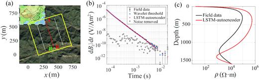
(a) Configuration of the transmitter–receiver device used in the field experiment. Transmitter loop source and receivers are shown by the thick yellow line and dots, respectively. The red star in the inset map in the upper left corner represents the geographical location of the field experiment. The TEM data measured at receivers and corresponding inversion results along line AB (red dots) are presented in Fig. 14. (b) Field TEM data (black dots) collected by receiver R (green dot) in (a) and de-noised results by wavelet threshold method (blue dots) and the LSTM-autoencoder (red dots). Grey dots show the difference between the original field data and the de-noised results by the LSTM-autoencoder. (c) Inversion results from signals in (b).
Fig. 14 shows the comparisons between the de-noised results and corresponding original field data, together with the inversion results. Fig. 14(a) displays the collected field data arranged according to the spatial positions of the receivers along Line AB (Fig. 13a). Although the data has been stacked and filtered by the instrument, it still has a high level of noise after 5 ms. Fig. 14(b) displays the de-noised TEM data, where the noise is effectively removed and the responses decay smoothly in time. The time range of the field data that can be used in further analysis has been extended from ∼5 to 21 ms, which is a significant enhancement in the data availability and will definitely contribute to the interpretation at greater depth. The excellent de-noising performance also demonstrates that the noises we used in the synthetic experiments in Section 3.1 are representative of the realistic ambient noise environment. To illustrate the effect of de-noising on the underground structure imaging, the inversion results from the original field data as well as the de-noised data are shown in Figs 14(c) and (d). The image in Fig. 14(c) shows discordant models between adjacent receivers with little horizontal structural coherency and poor resolution of the low-resistivity layer at around 1400-m depth. After the LSTM-autoencoder de-noising operation, the inversion results show a more horizontally coherent structure with clearer resistivity interface and achieve a better global data fit with the RMSPE dropping from 7.33% to 1.59%. Our result demonstrates that the output by the LSTM-autoencoder can obtain a more stable and reliable resistivity structure at a greater depth.
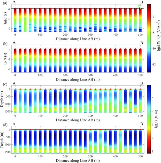
(a) Field TEM data along line AB (Fig. 13) as a function of distance and transient time. The red dots indicate the 26 receivers with equal spacing of 20 m. The green dot shows the location of receiver R. (b) De-noised TEM data from the LSTM-autoencoder. (c) 1-D resistivity models beneath the receivers obtained from field TEM data in (a) with a global data fit RMSPE of 7.33%. (d) Same as (c) but obtained from de-noised TEM data in (b) with an RMSPE of 1.59%.
Note that Phoenix V8 field data are only recorded until 21.3 ms at a minimum induced voltage of approximately |${10^{ - 12}}\,{{\rm{V}}}\,{{{\rm{A}}^{-1}\,{{\rm{m}}^{-2}}}}$| at later times. These are rather normal in loop source TEM experiments. Longer transients were not obtained during the survey to save acquisition time and considering that the field data were already affected by the noise at around 1 ms with standard instrumental processing. However, if trained sufficiently, the LSTM-autoencoder is capable of de-noising the data of longer than 20 ms. Future studies with optimal TEM survey designs are desirable to verify LSTM-autoencoder de-noising capabilities for longer time ranges using larger-scale set-ups.
5 CONCLUSIONS
In this study, we have developed a new architecture of neural network to suppress noise in TEM data. It is based on the LSTM memory blocks and autoencoder structure. A trained LSTM-autoencoder is only strictly valid for the signals generated by the same mechanism as the training data set, and the effectiveness of de-noising relies on the training duration and sample completeness. We use multiple types of noises and a large number of sample data sets in training the network in order to enhance its adaptability to real noise environments. Besides, LSTM-autoencoder is able to de-noise newly acquired data sets directly by learning the implicit relationships between data with and without noise in the training data sets, without additional efforts such as spectrum analysis. The LSTM-autoencoder shows a stronger adaptability to a variety of noises among several conventional de-noising techniques. Comparing with other commonly used networks such as the autoencoder, the FC and LSTM networks, the LSTM-autoencoder achieves the smallest errors for the test set and the de-noised results are much closer to the noise-free signals. Synthetic inversion experiments demonstrate that the resistivity structures obtained from data sets de-noised by the LSTM-autoencoder also agree best with the original model. In addition, an application to field data shows that after processing by the LSTM-autoencoder the noise is removed effectively, despite using synthetic training samples, and achieving a structure imaging with higher resolution at greater depths. Results presented here suggest that the LSTM-autoencoder can be used to address TEM de-noising challenges and ensure the quality of the data sets, which is important for improving the resolution in the inversions for subsurface resistivity structures.
ACKNOWLEDGEMENTS
This study was supported by the National Natural Science Foundation of China (41874082). We thank Shunguo Wang and Pritam Yogeshwar for their constructive comments. The authors also acknowledge the course ‘English Composition for Geophysical Research’ of Peking University (Course #01201110) for help in improving the manuscript. All synthetic data generated or used during the study are available from the corresponding author by request and field data sets are proprietary or confidential in nature and may only be provided with restrictions.
