


SUMMARY
To produce the electromagnetic (E&M) precursors of an earthquake, the existence of electric field due to stress-induced charges on the ground surface or in shallow depths of upper crust inside the fault zone is a basic condition. Here, we consider the piezoelectric effect or the elastic–electric coupling as a major mechanism on generating such an electric field. A 1-D model based on the elastic mechanics and electromagnetic Maxwell equations is built up to formulate the relationship between electric field and slip as well as stress on a fault before an earthquake. From the model, we may estimate the low-bound values of stress and slip to yield the critical electric field, Ec, for generation of electromagnetic signals. The normal and shear stresses on the fault planes for three faulting types are constructed. The normal stress is stronger than the shear stress to result in piezoelectricity. The depth ranges for yielding an average normal stress being able to generate Ec are similar for thrust and strike-slip faults and deep for normal faults. The possibility of generating Ec is almost the same for thrust and strike-slip faults and low for normal faults. The pre-earthquake slip could be related to nucleation phases or microfractures. The possible occurrence time of E&M signals may be several 10 min to few hours before impending earthquakes. The major factor in yielding a piezoelectric field to generate the TEC anomalies before an earthquake is the existence of fault gouges composed mainly of clays. A thick gouge layer with low electric resistivity and a piezoelectric coupling coefficient ≥0.67 × 10⁻¹² coul nt–1 is an important condition for yielding piezoelectricity.
1 INTRODUCTION
Anomalous electromagnetic (E&M) signals have been detected in the Earth's crust, Earth's ground, the atmosphere and ionosphere over an area covering the earthquake source in a short time, for example several hours to few days, before an impending event. The ground-based observations of E&M signals include thermal anomaly (e.g. Ouzounov et al. 2006), anomalous electric resistivity and conductivity (e.g. Du et al. 2015), geomagnetic fluctuations (e.g. Han et al. 2016), ionospheric sounding (e.g. Liu et al. 2010), DC electric field emissions/ULF/VHF (e.g. Uyeda et al. 2009), amplitude and phase anomalies of subionospheric VLF/LF signals from powerful transmitters (e.g. Hayakawa et al. 2012) and variations in total electron content (TEC, e.g. Heki 2011). The satellite data also reveal wave and plasma disturbances before earthquakes (e.g. Li & Parrot 2013). These phenomena include the presence of electron density fluctuations in the ionosphere above the earthquake source areas (e.g. Liu et al. 2009; Heki 2011), the change of ionic composition and temperature of plasma in the ionosphere (e.g. Ho et al. 2013), and oscillation of the height profile of the ionospheric F region (e.g. Cahyadi & Heki 2013).
Actually, it is necessary to build up a comprehensive model for the lithosphere–ocean–atmosphere–ionosphere coupling to interpret the E&M precursors. Several proposed models are: (1) a model to present radon ionization and charged aerosol and change of load resistance in the global electric circuit (see Pulinets & Ouzounov 2011; and cited references therein); (2) a model to show coupling between stressed rocks and the atmosphere–ionosphere system (e.g. Kuo et al., 2011, 2014) based on experimental results of stress-induced charges made by Freund (2002); (3) a model to display ionosphere dynamics with imposed zonal (west–east) electric field (Zolotov et al., 2011, 2012; Namgaladze et al. 2012) and (4) leakage of electric currents from ocean into the crust having low electric resistivity (Madden & Mackie 1996).
It needs a physical mechanism which could generate electric charges on the Earth's ground or in the uppermost crust for the need of above-mentioned models. Several mechanisms, including rock fracturing by bending moment (Ogawa et al. 1985), streaming potentials (e.g. Bernard 1992), piezoelectricity (e.g. Bishop 1981; Ogawa & Utada 2000a), piezomagnetism (e.g. Sasai 1979), triboelectricity/triboluminescence (e.g. Yoshida et al. 1998), spray and contact electrification, confined pressure changes (e.g. Fujinawa et al. 2002) and microfracturing (e.g. Molchanov & Hayakawa 1995) have been applied to explain charge generation inside and near faults. Nevertheless, Freund (2002) argued that some of these processes cannot represent a coherent physical model to simultaneously interpret the electrical, electromagnetic and luminous phenomena. From the laboratory experiments of crystalline physics, Freund (2000) found that water molecules embedded in rocks can dissociate into ions if the rocks are under strong stresses and the resulting charge carriers can generate currents under certain conditions. He assumed that these currents could be responsible for some E&M precursors. Meanwhile, he proposed the peroxy defect theory to explain the experimental results and also suggested that rocks may contain charge carriers which can be identified from field data.
Although the experimental results and physical model made by Freund and his coworkers are actually excellent, some basic problems about their suggestion that stress-induced signals can be detected and used as a precursor should be concerned. First, rock mechanics experiments reveal that the stress loaded on a fault first increases, reaches its peak, and then decreases with increasing time before a large earthquake. (This phenomenon will be described in details below.) Hence, the largest currents related to the strongest loaded stress might be generated several months to several years before an impending earthquake and then decrease until the event occurs, because the peak loaded stress happened several months to several years before the event, especially for large earthquakes. This is questionable because E&M signals are usually observed only in a short time before an event. For example, the TEC anomalies appeared about 40–100 min before earthquakes with Mw > 8 and 10 to 20 min before earthquakes with Mw 7–8 as pointed out by Heki and his coworkers (e.g. Heki 2011). Secondly, Freund and his coworkers used pure granite in their experiments. However, in the fault zone the materials are quite complicated even though granite is the main component. Thirdly, it is questionable if the stress loaded on a fault plane is strong enough, especially in the shallow crust, to generate charges. This point will be discussed in details below. Hence, it is significant to explore the possible mechanism for generating the electric field/current from an alternative viewpoint.
Piezoelectricity or elastic–electric coupling (EEC, see Fig. 1), which was first found by two French physicists Jacques and Pierre Curie in 1880, means that when a stress is applied to some crystals in certain crystallographic directions, opposite sides of the crystals become instantly charged (cf. Kittel 1971; Finkelstein et al. 1973). Freund (2002) asserted that this effect is not appropriately used for charge generation by stresses, because the piezoelectric potentials tend to cancel when quartz crystals distribute in random orientation in a stressed volume. Nevertheless, I still assume that for stress-induced charges, EEC is an acceptable macroscopic model and the peroxy defect theory the microscopic one. Quartz is abundant in the Earth's crust and the mineral in a piezoelectric symmetry class. For the generation of a natural earthquake, the piezoelectric effect could exist because the stresses loaded on a fault are not random. The fault gouge is the most possible candidate for stress-induced charges and the reasons will be given below.
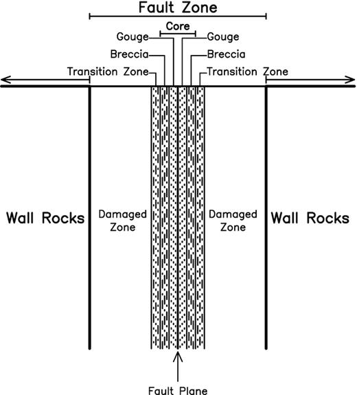
A simplified, non-scaled diagram to schematically describe the fault-zone structure. (modified from Choi et al. 2016).
On areas specified with highly active deformation of the Earth's crust, especially the upper crust, the ability of transforming mechanical energy into E&M waves would play a significant role on the generation of short-term precursors, for examples, geomagnetic and TEC anomalies. An important problem in seismo-electromagnetic research is: Can pre-earthquake slip generate the ground surface electric field/current?
This problem is related to the physical processes, water, and materials in the fault zone. In order to resolve the problem, four research issues will be conducted below. First, according to the idea pointed out by Sornette (2001) a working model based on piezoelectricity will be proposed to connect the electric field with loading stress as well as slip. Secondly, we will combine piezoelectricity and mechanical behaviour (including geometry and mechanics of loading stresses) of the fault zone to explore the depth range, which depends on faulting type and static friction coefficient, to yield a large enough normal stress for inducing charges in the uppermost crust, thus generating E&M signals (mainly the TEC anomalies). Thirdly, based on the temporal variations in stress and stress intensity obtained from laboratory experiments on rock mechanics we will search for the most possible occurrence time of E&M precursors, especially for the TEC anomalies. Fourthly, the candidate material and physical conditions for inducing charges will be identified based on the electric properties and thicknesses of fault-zone materials.
2 FAULT-ZONE STRUCTURE
The fault zone extends from the ground surface to the depths of several to several tens kilometers. There are three sections of a fault zone in different depth ranges with different materials: Section 1 consisting mainly of gouges and breccia in the depth range 0–3 km; Section 2 composed mainly of cataclasite from ∼3 to ∼10 km; and Section 3 having mylonite below ∼10 km or deeper. The temperature is <100 °C in Section 1, between 100 and 300 °C in Section 2, and > 300 °C in Section 3. Brittle fracture happens in Sections 1 and 2; while ductile deformation works in Section 3. As discussed below, this study will focus on the uppermost almost one kilometers of the crust. Hence, only the first depth range is considered. The shallow fault zone as displayed in Fig. 1 is composed mainly of fault core, transition (or alternation) zone, and damage zone from the fault plane to outside (Choi et al. 2016). Outside the damage zone are wall rocks whose displacements and fractures during faulting are much smaller than those in the fault zone.
Wear caused by frictional sliding can result in damage and erosion on the sliding surfaces (Rabinowicz 1965). Abrasive wear and adhesive wear are particularly important in the fault zone (Scholz 1990). Since the latter that plays a main role only in Section 3 with ductile or plastic deformations, it is not further described hereafter. The former is important in Sections 1 and 2 of a fault zone and its mechanism is that due to a hardness contrast between opposite materials of the fault plane, the harder material may plough through the softer material out. For brittle rock-forming matters, the abrasive wear will be dominated by brittle fracture, thus yielding gouge which are loose wear particles with angular forms. Based on the wear theory (Archard 1953) and laboratory results (Logan & Teufel 1986), Scholz (1987) correlated the gouge thickness, hg, to fault slip, u, as hg/u= (α/3Hp)σn, where α, Hp and σn are, respectively, the dimensionless parameter, hardness parameter of material, and normal stress. (Hp and σn have the same unit, Pa or MPa.) Clearly, the ratio hg/u increases with σn with a slope of α/3Hp that depends on the material. From the data obtained by Yoshioka (1986), Scholz (1987) inferred that the value of α/3Hp is higher for (softer) sandstone than for (harder) granite. Consequently, long u and high σn yield thick hg.
The main materials of a fault core whose width varies from several ten centimeters to few hundred centimeters are breccia and gouges. Although gouges and breccia are mainly distributed, respectively, in the central part and in the outer part of a fault core as displayed in Fig. 1, they may be intermingled. The width of damaged zone in each side to the fault plane is about several ten meters. There is a question: Does piezoelectricity occur in the whole fault zone or merely in the fault core? Actually, it is not easy to answer the question exactly this time. But, I assume that piezoelectricity occurs merely in the fault core, because the damaged zone is actually the fractured rocks caused by an earthquake and did not deform before the event. In addition, it may be easier to produce piezoelectricity in a narrow range like the fault core than in a wide one like the whole fault zone.
Gouges that are mainly composed of clays (Scholz 1990) have a very small grain size and are incohesive and usually unconsolidated. Clays are finely grained rocks or soils that consists of a material or combine several minerals [including quartz (SiO2), metal oxides (Al2O3, MgO etc.) and organic matters] together. Since a gouge-filled fault is commonly weak, strong enough compressive stresses loaded on it can cause compressive yielding or eventually fracture (Bertuzzi 2015). Breccia is a clastic sedimentary rock that is shaped from angular and boulder size clasts cemented or in a matrix. The presence of angular shape show that a clast with a grain size >2 mm has not been transported from its source. Breccia is an incohesive, crushed rock composed of broken fragments of minerals resulted from grinding of two fault blocks that move past each other or are cemented together by a fine-grained matrix. Sibson (1977) observed that gouges have less (<30 per cent) visible fragments than breccia (>30 per cent). The latter is usually outside and thicker than the former. The degree of cohesion of gouges and breccia will be increased due to cementation taking place at a later stage of faulting. Subsequent cementation of these broken fragments may occur by means of the introduction of mineral matter in groundwater.
3 PRINCIPLE OF PIEZOELECTRICITY
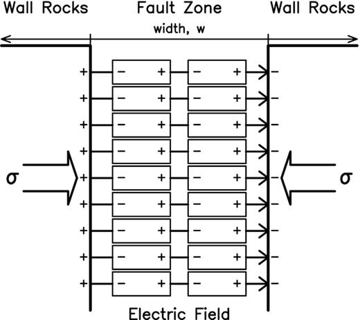
Schematic description of piezoelectric effect or elastic–electric coupling.
4 TEMPORAL VARIATIONS IN STRESS ON A FAULT BEFORE AN EARTHQUAKE
The stress σ usually varies with time (Atkinson 1984; Rudnicki 1988; Main & Meredith 1989) as schematically displayed in Fig. 3(a). There are three stages, that is Stages 1–3, before an earthquake (at t = tr) and two stages, that is Stages 4–5, during and after the event. In general, the time period is the longest (several 10 or hundred years) in Stage 1 from to to ty and the shortest (several 10 s) in Stage 4. In Stage 1 elastic buildup of strain energy starts at to and stops at ty when the elastic (linear) loading transfers to plastic (non-linear) loading, thus yielding the long-term precursors such as a seismic gap. The changing point from elastic loading to plastic loading is called the yielding point. Stage 2 (occurring from ty to tm when the loading stress reaches its peak) displays plastic strain hardening due to dilatancy because of crack coalescence and fluid transport in the fault zone. The time period of this stage is several years. Intermediate-term precursors, such as the b-value anomalies, may be observed in this step. In Stage 3 (occurring from tm to tr) the loading stress decreases and demonstrates precursory stress drop or strain softening. The time period of this stage is several months. Stage 3 has three steps (3a, 3b and 3c): (3a) for microcrack linkage, (3b) for pore fluid diffusion and (3c) for quasi-static slip on the fault between asperities. The mechanic behaviour in this step could result in short-term and imminent precursors such as the non-volcano tremors (e.g. Katakami et al. 2018) due to microcrack linkage, the water-level change in wells caused by pore fluid diffusion, and foreshock activity and E&M signals induced by quasi-static slip. Field observations (e.g. Jones & Molnar 1979; Fujinawa et al. 2002; Lin 2009; Papadopoulos & Minadakis 2016) show that several days prior to an impending main shock, foreshock activity or microcracks starts to increases and rapidly accelerates in the last day within the surrounding area with distances smaller than a certain value, for example 30 km, near the main shock epicentre. In Stage 4 the asperities on the fault break at time tr and then the earthquake ruptures during a short time interval after tr, thus resulting in dynamic slip of the fault behind the crack tip. In Stage 5 aftershocks, which may last for several months or longer, yield transient stimulation of further stress drop in the source area.
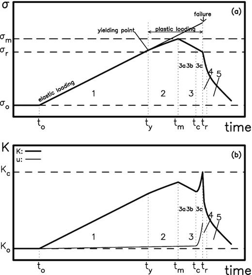
The temporal variations in stress, σ, stress intensity, K and slip, u, in a fault zone: (a) for σ and (b) for K (thick line) and u (thin line). The detailed description concerning this figure can see the text (modified from Main & Meredit 1989).
In eqs (20) and (21), uo and uto are, respectively, the initial crack length and initial crack velocity. Eq. (21) is displayed by a thin solid line in Fig. 3(b). A detailed description about dependence of u on n is given in Fig. 8 and discussed below. The u increases very slowly with time before Step 3c and then increases abruptly with time within this sub-step until failure of an event. The K increases with time and reaches its local maximum at time tm, then decreases with increasing time, and increases again to Kc within Step 3c. In Step 3c, σ decreases with increasing time and K increases with time due to a remarkable increase in u that compensates a reduction in σ.
5 DISCUSSION
5.1 Piezoelectric strengths and related mechanisms
From eq. (13), the strength of the EEC wave is represented by (μ/χ)ζ2. For quartz, (μ/χ)ζ2 is ∼3 × 10⁻³ because of χ= 4.5χo (χo = 8.854 × 10⁻¹² F m-1), μ ≈ 30 GPa and ζ = 2 × 10⁻¹² coul nt–1. This suggests weak EEC. The amplitude of the E&M (fast) mode is given by eq. (16), namely χE = –ζσn in absence of preexisting electric field, that is I = 0. Using χ= 4.5χo and ζ= 2 × 10⁻¹² coul nt–1, we obtain |E| ≈0.05σ., thus giving E ≈ 5 × 10⁵ V m–1 when σ = 10 MPa. Although ζ= 2 × 10⁻¹² coul nt–1 is the common value of granite (cf. Sornette 2001), the values of ζ for some granites may be smaller than the common one. For example, Sasaoka et al. (1998) experimentally obtained ζ = 1.4 × 10⁻¹⁵ coul nt-1 for granite samples from Fujian, China. They also claimed that this value is actually three orders of the magnitude smaller than 2 × 10⁻¹² coul nt–1. Based on their experimental value, we have (μ/χ)ζ 2 ≈ 1.476 × 10⁻¹⁰, thus suggesting very much weak EEC. Considering ζ = 1.4 × 10⁻¹⁵ coul nt–1, we have |E|≈3.76 × 10⁻⁵σ, thus giving E ≈ 3.76 × 10² V m–1 when σ=10 MPa.
Kuo et al. (2011, 2014) claimed that the typical values of the dynamo current J used in their calculations for generating the total electron content (TEC) in the ionosphere are 1–100 nA m–2. For J = 10 nA m–2, the related electric field on the Earth's ground surface is E = 5 × 10⁵ V m–1. This suggests that σ=10 MPa related to ζ=2 × 10⁻¹² nA m–2 could be a lower bound stress for yielding a significant piezoelectric field. Meanwhile, E = 5 × 10⁵ V m–1 is considered to be the critical electric field in this study and denoted by Ec hereafter. Since the stress is almost zero on the ground surface, the piezoelectric field must be produced in a depth range of the crust.
Eq. (16) leads to |E+|=(c/v)2(κ/ζ)|u+|, thus showing that longer u+ results in stronger E+. Inserting the values of c and ζ as mentioned previously and v = 600 m s–1 for shallow crust into this expression gives |E+|=1.25 × 10²³κ|u+| (in V m–1). This expression can be rewritten as |E+|=7.854 × 10²³|u+|/λ (in V m–1) because of κ=2π/λ. For |E+|=Ec = 5 × 10⁵ V m–1, we have |u+| = 6.366 × 10⁻¹⁹λ (in m). From Heki (2011), we can see that the TEC anomalies start almost 40 min before the 2011 Tohoku-Oki earthquake. The ending time is variable. Their studies reveal that the anomalies observed by satellite 26 seem to stop ∼10 min after the earthquake due to the hole generation. However, other satellite data, for example, the data from satellite 15, show that the anomalies gradually decay starting immediately after earthquake and taking 10–20 min. This means the duration time of TEC anomalies is, at, least, T ≈ 50 min or 3.0 × 10³ s and thus the related wavelength is λ = cT ≈ 8.997 × 10¹¹ m because of c = 2.999 × 10⁸ m s–1. This gives uc = |u+| = 5.727 × 10⁻⁷ m, which is the critical slip to yield Ec for triggering TEC anomalies. As displayed in Fig. 3(b), u+ (denoted by u in the figure) increases very slowly with time from Stage 1 to Stage 3 and then abruptly increases in Step 3c. Nevertheless, the value of u should be very small before failure of a fault.
The pre-earthquake slip for larger-sized events may be associated with four seismic phenomena: (1) foreshocks (e.g. Jones & Molnar 1979; Lin 2009); (2) the slow earthquakes (including deep episodic tremor, low-frequency earthquakes, very-low-frequency earthquakes, slow slip events and silent earthquakes, e.g. Ide et al. 2007; Kano et al. 2018; Nishikawa & Ide 2018); (3) the nucleation phases (e.g. Umeda 1990; Ellsworth & Beroza 1995; Mori & Kanamori 1996; Wang 2017) and (4) microfracturing (e.g. Molchanov & Hayakawa 1995). These seismic phenomena could represent four mechanisms on generating the electric fields for E&M signals.
For the first seismic phenomenon, it is significant to consider average slip of the largest-sized foreshock of a main shock. The moment magnitude, Mw, of an event is correlated to the average slip, ū, on its source area. Based on the u–L relationships (L = fault length) and the Mw–L relationships inferred by Wells & Coppersmith (1994), we can obtained Mw = 6.16 + 1.66log(ū). The relationship between the moment magnitude (denoted Mwm) of a main shock and that (denoted by Mwf) of its largest- sized foreshock is not yet known. Jones & Molnar (1979) compiled a large number data of Mwm and Mwf and then plotted them on a diagram. Their results show three interesting phenomena: (1) the difference Mwm–Mwf varies from 0 to 3; (2) the difference increases with Mwm and (3) the difference is remarkably larger than 1 when Mwm ≥ 8. Considering a main shock with Mwm = 8.0, the value of ū of its largest-sized foreshock with Mwf = 7 is ∼2.43 m from the above-mentioned scaling law. Hence, we have |E+|=7.634 × 1024/λ (in V m–1). In order to obtain |E+|=Ec = 5 × 10⁵ V m–1, the modelled wavelength λ is 1.527 × 10¹⁹ m and thus the related period T is 5.092 × 10¹⁰ s because the wave propagates with light speed. There are five problems. The first one is that the modelled wavelength is too long. For the 2011 Mw 9.0 Tohoku‐Oki, Japan, earthquake, the fault length is ∼400 km or ∼4.0 × 10⁵ m (cf. Lee et al. 2011). Hence, the modelled wavelength is 3.818 × 10¹³ times longer than the fault length. From the observations by Heki (2011), the duration time, T, of TEC anomalies for the earthquake is ∼55 min or 3.3 × 10³ s and thus the modelled period is 1.543 × 10⁷ times longer than observed duration time of TEC anomalies. The two things do not seem reasonable and it is also difficult to explain the big differences. The second one is that the largest-sized foreshock could not result in a detectable electric field because its focal depth is usually deep. The third one is: Observations reveal that foreshocks happen mainly before normal and strike-slip earthquakes and very few even none before thrust ones. This would be not good for some seismically active regions, for examples Taiwan and Japan, where earthquakes are mainly caused by thrust faulting. The fifth one is: Foreshocks usually occur a few days before the main shocks. This is inconsistent with the occurrence time of TEC anomalies as reported by Heki (2011) and his coworkers. Hence, I do not think that foreshocks produce the pre-earthquake electric field.
For the second seismic phenomenon, from Table 1 of Ide et al. (2007) we can see that the average displacements of slow slip earthquakes (SSE) are 10−3 to 1 m, which are much longer than 6.873 × 10⁻⁷ m, occurred several to several ten days before main shocks. From the Hi-net tiltmeters Obara et al. (2004) and Hirose & Obara (2005) detected the tilt deformations caused by SSE before main shocks in the southwest Japan subduction zone. In case that the pre-earthquake slip is produced by SSE, the E&M signals should be very strong and happen several or several ten days before the main shocks. This is inconsistent with the occurrence time of TEC anomalies as reported by Heki (2011) and his coworkers. In addition, from the tiltmeter array in NE Japan, Hirose (2011) claimed that pre-seismic tilt change or pre-seismic slip was not found in the records before the 2011 Mw 9.0 offshore Tohoku earthquake. This indicates that there is no interplate pre-slip larger than Mw 6.2 on the deeper extension of the earthquake source area on the interface along the subducting Pacific Plate or larger than Mw7.3 near the hypocentre. Obviously, SSE does not occur anywhere. Hence, this mechanism can be given up.
The fault name, magnitude of occurred earthquake (Mw), fault-core thickness (hc), fault-gouge thickness (hg), electric resistivity (Re), average slip (ū), maximum slip (umax) and detection of TEC anomalies (TA; y = reported by some authors; n = not confirmed by Heki and his coworkers) for faults in this study.
| Faults | Mw | hc (m) | hg (m) | Re (Ω-m) | ū (m) | umax (m) | TA | Remarks |
|---|---|---|---|---|---|---|---|---|
| Tohoku-Oki | 9.0 | <10 | <4.86 | <2.5 | 18 | 50 | y | hc, h and Re from Chester et al. (2013) |
| ū and umax from Lee et al. (2011) | ||||||||
| Longmenshan | 7.9 | ∼2.54 | ∼0.54 | ∼20 | 2.23 | 12.5 | y/n | hc and h from Kuo et al. (2017) |
| Re from Li et al. (2013) | ||||||||
| ū and umax from Wang et al. (2008) | ||||||||
| Chelunngpu | 7.6 | ∼1.2 | 1.12 | 6.9 | 1.8 | 16 | y/n | hc, h and Re from Hung et al. (2009) and Wu et al. (2008) |
| ū and umax from Lee et al. (2006) | ||||||||
| Nojima | 6.9 | ∼1 | 2 | 2.1 | 3.47 | y/n | hc from Lockner et al. (2009) | |
| Re from Sumitomo et al. (1997) | ||||||||
| ū from Kikuchi & Kanamori (1996) | ||||||||
| umax from Wald (1996) | ||||||||
| San Andreas (near Parkfield) | 6 | 2.5 | ∼10 | Morrow et al. (2015) | ||||
| Olkhon | ? | ∼50 | <230 | Seminsky et al. (2016) |
For the third seismic phenomenon, nucleation phases are observed by seismometers in a short time span before an earthquake. Mori & Kanamori (1996) observed that the rupture velocity of nucleation phases is lower than 10−4 m s–1 in a time span of 0.05 s occurred about 0.05 s before an earthquake, and then rapidly increases until the earthquake happens. Thus the displacement at 0.05 s is shorter than 5 × 10⁻⁶ m which is longer than the critical slip |u+|=uc = 6.873 × 10⁻⁷ m. The pre-earthquake slip may be equal to the critical value much earlier. Mori & Kanamori (1996) also suggested that any radiation at seismic frequencies prior to an earthquake must emanate from a source region with a dimension smaller than ∼10 m which is the fault length of a M0.5 event. Hence, the pre-earthquake nucleation could be a possible mechanism on the generation of ground electric field.
For the fourth seismic phenomenon, the critical displacement uc = 5.727 × 10⁻⁷ m is comparable with the size of random defects (10−6–10−7 m) of microfractures in rocks (Makklintok & Argon 1970; Molchanov & Hayakawa 1995). Microfracturing is considered a common phenomenon in Step 3c as mentioned above. In addition, Molchanov & Hayakawa (1995) assumed that microfracturing is the mechanism of generation of ultra-low frequency (0.01–10 Hz) E&M emissions. Hence, microfracturing may be a mechanism on generating electric fields. Of course, more studies, including the use of a 2-D model, should be done to deeply explore the influences of nucleation and microfracturing on pre-earthquake slip for generation of electric fields.
5.2 The depth range for producing piezoelectricity in a fault zone
In order to understand how EEC functions in a fault zone prior to an earthquake, it is necessary to consider the geometrical structure of stresses on faults, including thrust, normal, and strike-slip faults (see Fig. 4). The detailed description about the geometrical structures and mechanics of stresses can be seen in Turcotte & Schubert (1982). A simple description is given in Appendix B. As displayed in Fig. 4, there are three stresses, σ1, σ2 and σ3 loading on a fault. Two of the three stresses depending on faulting type may be composed to produce the normal stress, σn, which is perpendicular to the fault, and the shear stress, σs, which is along the fault.
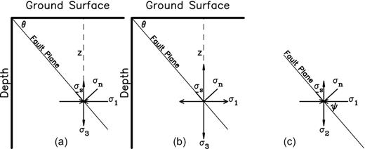
The geometrical structures of stresses for three types of faults: (a) for thrust fault, (b) for normal fault and (c) for strike-slip fault. The depth is denoted by z. The principal stresses along the horizontal vertical axes are σ1 (=ρgz) and σ3, respectively. The σn and σs represent the normal stress and shear stress, respectively. The thrust and normal faults have a dip angle of θ. The strike-slip fault is inclined to the direction of σ1 is ψ.
Both σn and σs may induce the electric field (see Kittel 1971). The shear stress behaves also like friction, which could result in triboelectricity as proposed by Yoshida et al. (1998). Coseismic ionospheric disturbances (CID) after large earthquakes are the superposition of perturbations by different origins such as coseismic vertical crustal movements (Heki et al. 2006; and cited references herein); propagating Rayleigh surface waves (e.g. Artru et al. 2004); propagating teleseismic body wave (Ogawa & Utada 2000b); and internal gravity waves due to tsunamis induced by submarine earthquakes (e.g. Liu et al. 2006). Hence, CID depends on the origins and the distance from the epicentre. For near-field CID, Astafyeva & Heki (2009) studied TEC responses, recorded at numerous GPS receivers, to three large earthquakes that occurred in the Kuril Arc on October 4, 1994 with high-angle reverse faulting, 15 November 2006 with low-angle reverse faulting, and 13 January 2007 with normal faulting. The initial TEC changes at different receivers are positive for the 2006 event and negative for the 2007 event; while those for the 1994 event have both positive and negative polarities depending on the azimuth around the focal area. They assumed that such a variety may reflect different dominated coseismic vertical crustal displacements: uplift in the 2006 event, subsidence in the 2007 event, and both in the 1994 event. Cahyadi & Heki (2015) compared CID amplitudes of 21 world-wide earthquakes with Mw 6.6–9.2. Out of them, eighteen events were thrust faulting, two events normal faulting, and one strike- slip faulting. Their results show that CID amplitude, ACID, roughly scales with Mw in a form of ACID∼Mw2/3. But, the data point of 2012 North Sumatra earthquakes slightly deviated negatively from the trend. This may reflect their strike-slip mechanisms, whose vertical crustal movements were small. The two studies indicate the importance of vertical slip due to σs on near-field CID. Clearly, σs plays a minor role on the E&M signals before earthquakes due to small pre-earthquake vertical slip.
For thrust and normal faults, eqs (B3) and (B10) give σn = σL+ σT[1–cos(2θ)]/2 = σL+σT[1–fs/(1 + fs2)1/2]/2, where σL =ρgz is the lithostatic pressure at depth z, σT is the tectonic deviatoric stress, θ is the dip angle of the fault and fs is the static friction coefficient on the fault. For strike-slip faults, eqs (B6) and (B13) yield σn = σL– σTcos(2ψ)= σL– σTfs/(1 + fs2)1/2, where the fault is inclined at an angle ψ to the direction of σ1. Eqs (B4) and (B10) lead to |σs|=|σTsin(2θ)|/2=|σT/(1 + fs2)1/2|/2 for thrust and normal faults and eqs (B7) and (B13) give |σs|=|σTsin(2ψ)|/2=|σT/(1 + fs2)1/2|/2 for strike-slip faults. As explained in Appendix B, the values of fs range from 0 to 0.85. From these equations, we can see |σs|<|σn|. Nevertheless, it is still necessary to quantitatively explore if σs can be ignored for EEC or not.
Eq. (B11) gives σT= ±2fs(σL–pw)/[(1 + fs2)1/2–(±fs)], where pw is the pore fluid pressure and the upper and lower signs of ‘±’ are used for thrust faults and normal faults, respectively. Eq. (B14) leads to σT = fs(1 + fs2)1/2(σL–pw)/(1–fs2) for strike-slip faults. From Appendix B, pw (=λvσL) is ∼0.4ρgz. The ratio |σs/σn| for three faulting types is displayed in Fig. 6: a dashed line for a thrust fault, a dashed–dotted line for a normal fault, and a solid line for a strike-slip fault. This figure shows that |σs/σn| increases with fs for the three faulting types. However, the increasing rate of |σs/σn| with fs is higher for thrust faults than for normal and strike-slip faults. The values of |σs/σn| are in the range 0–0.605 for thrust faults, 0 to 0.166 for normal faults, and 0 to 0.198 for strike-slip faults when fs varies from 0 to 0.85. This suggests that the electric field is weaker from σs than from σn, especially for normal and strike-slip faults. Hence, only EEC caused by σn on a fault is taken into account hereafter. In general, the effect due to exclusion of σs on EEC is small for normal and thrust faults with fs ≤ 0.85 and for thrust faults with low fs, but large for thrusts with high fs. In addition, the effect due to σs may be ignored when pw is high enough to yield a low effective friction coefficient. In order to include EEC caused by σs, especially for thrust faults, a 2-D model should be considered. This will be done in the near future.
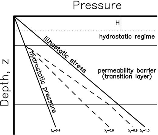
Schematic diagram for underground stress system: the right inclined line representing the depth-increasing lithostatic stress, the left line denoting the depth-increasing hydrostatic pressure with λv = 0.4; two dashed lines showing two examples (λv = 0.6 and 0.9) of increases in hydrostatic pressures due to the permeability barrier (or transition layer) which is located in between two horizontal lines (∼2 km for the upper line and ∼6 km for the lower one). The depth range in between the ground surface and a depth of H expresses the range within which the loaded stress can yield the strong enough electric field for generating E&M precursors as discussed in the text. (modified from Sibson (1977) and Zencher et al. (2006)).
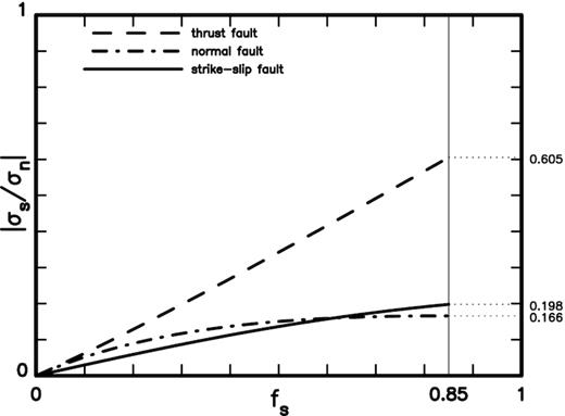
The ratios of |σs| to |σn| for three faulting types: a dashed line for thrust fault, a dashed-dotted line for normal fault, and a solid lines for strike-slip fault. The thin vertical line represents fs = 0.85.
Eqs (22)–(24), Ho = 2σna/ρg is the depth associated with fs = 0.0. The gradient of σL with depth is ρg whose average value is ∼27.5 MPa km–1 in the Earth's crust (Turcotte & Schubert 1982). For Ec = 5 × 10⁵ V m-1, σna = 10, 30 and 60 MPa that arenrelated to ζ=2 × 10⁻¹², 0.67 × 10⁻¹² and 0.35 × 10⁻¹²coul nt–1, respectively, are taken into account. Hence, Ho is 727.2 m for σna = 10 MPa, 2181.6 m for σna = 30 MPa and 4363.2 m for σna = 60 MPa. Based on eqs (22)–(24) with the respective values of Ho, the plots of H versus fs (0.0 ≤ fs ≤ 1.0) for the three values of σna are plotted in Fig. 7 where a dashed line is made for a thrust fault, a dashed–dotted line for a normal fault, and a solid lines for a strike-slip fault. In each diagram, a thin vertical line denotes the value of fs = 0.85 and two thin horizontal dotted lines display the permeability barrier (or transition layer, see Fig. 5), whose upper boundary has a depth of ∼2000 m and lower one has a depth varying from 3000 to 6000 m for different areas (Zencher et al. 2006). For σna = 10 MPa, H is 510.6–727.2 m for thrust faults, 727.2–1263.1 m for normal faults and 582.4–727.2 m for strike-slip faults. For σna = 30 MPa, H is 1531.7–2181.6 m for thrust faults, 2181.6–3789.2 m for normal faults and 1747.3–2181.6 m for strike-slip faults. For σna = 60 MPa, H is 3063.5–4363.2 m for thrust faults, 4363.2–7578.5 m for normal faults and 3494.7–4363.2 m for strike-slip faults.

The plots of H versus fs for three values of σna, that is 10, 30 and 60 MPa that are related to ζ=2 × 10⁻¹², 0.69 × 10⁻¹² and 0.35 × 10⁻¹²coul nt–1, respectively, for three faulting types: a dashed line for thrust fault, a dashed-dotted line for normal fault, and a solid lines for strike-slip fault. The thin vertical line represents fs = 0.85. The two horizontal dotted lines show the permeability barrier or transition layer as displayed in Fig. 5.
Considering σna = 10 MPa, H is shallower than 2000 m for three faulting types. This is almost a typical manner to yield EEC, thus generating E&M signals. The higher σna is, the deeper H is. Fig. 7 suggests that it is necessary to cover a wider depth range, especially for normal faulting, to include the permeability barrier to yield σna > 30 MPa. Two problems arise. The first problem is that high λv in the permeability barrier produces low σTa and thus low σna. In order to produce higher σna, there must be a wider depth range even covering the crust below the permeability barrier. This would not be beneficial for yielding EEC. The second problem is that there is a difference in electric resistivity, Re, between the hydrostatic layer and the permeability barrier. From Appendix B, the transition from the hydrostatic layer to the permeability barrier generally occurs due to crustal deformations of greenschist and higher grade metamorphic rocks. The values of Re of greenschist and higher grade metamorphic rocks are higher than those of the shallow fault-zone rocks that are mainly composed of gouge and breccia. Hence, Re should be higher in the permeability barrier than in the hydrostatic layer. This could reduce EEC, especially in the permeability barrier. Hence, Fig. 7 seems to suggest that σna = 30 MPa is the upper bound value and ζ=0.67 × 10⁻¹² coul nt–1 the lower bound value to yield EEC for generating the TEC anomalies. When ζ is smaller than 0.67 × 10⁻¹² coul nt–1 in a fault core, the piezoelectric field might be small or even cannot happen. Of course, this conclusion is made mainly based on the TEC anomalies. For some E&M signals near the ground surface, ζ could be smaller than 0.67 × 10⁻¹² coul nt–1. This needs more studies.
In addition, Fig. 7 also implicates two significant points. The first one is that it is more difficult to yield the piezoelectric field for normal faults than the others, because H is deeper for the former than the latter and increases with σn. In other words, it is more difficult to generate E&M precursors before normal faulting than before thrust and strike-slip faulting. The second one is that for thrust and strike-slip faulting, EEC is more easily generated for smaller fs than for larger fs, because H is deeper for the former than for the latter and increases with σn. The situation is totally opposite for normal faulting. Hence, it is easier to produce E&M precursors for lower angle thrust and normal faults than higher angle ones. For strike-slip faulting, it is easier to produce E&M precursors for smaller ψ , which is the inclined angle of a fault to the direction of σ1 (the maximum principal stress), than larger ψ.
5.3 Occurrence time of E&M signals
An abrupt increase in u remarkably strengthens E based on eq. (16). Heki (2011) found that TEC anomalies started ∼40 min before the 2011 March 11 Tohoku-Oki Mw 9.0 earthquake and reached nearly ten per cent of the background TEC. He also stressed that similar TEC anomalies, whose amplitudes depend on magnitudes of impending earthquakes, were observed before the 2004 Mw9.2 Sumatra-Andaman earthquake, the 2010 Mw8.8 Chile earthquake, and the 1994 Mw 8.3 Hokkaido-Tohoku- Oki earthquake, yet not in smaller earthquakes. Cahyadi & Heki (2013) added the 2007 Mw 8.5 Bengkulu, Southern Sumatra, earthquake. Heki & Enomoto (2015) further added the 2012 Mw 8.6 North Sumatra (Indian Ocean) earthquake, its largest Mw 8.2 aftershock, and the 2014 Mw8.2 Iquique earthquake. They also reported that the TEC anomalies occurred about 40–70 min before those earthquakes. He & Heki (2017) analysed vertical total electron contents (VTEC) recorded near the epicentres before and after 32 earthquakes with Mw7.0–8.0. Through rigorous examinations, they found that out of them eight events with Mw 7.3–7.8 showed pre-seismic anomalies starting 10–20 min before earthquakes. For earthquakes of this magnitude range, pre-seismic TEC anomalies are probably detected when the background VTEC is large, say 50 TECU (total electron content unit, 1 TECU = 1016 el m–2) or more. Their studies indicate that preseismic TEC anomalies occur only for few earthquakes with Mw ≤ 8 and the starting time is shorter than that for earthquakes with Mw > 8. In comparison with Fig. 3, their results strongly suggest that TEC anomalies appear only in the latest time span of Step 3c.
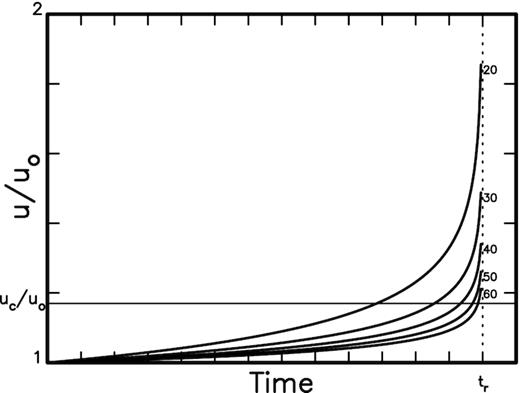
The plot shows the temporal variations in u/uo with time for five values of n, that is 20, 30, 40, 50 and 60. The thin horizontal line represents the ratio uc/uo whose uc is the critical value for producing a detectable electric field responsible for generation of ground electric currents.
Obviously, tc increases with n and the difference tr–tc = tr(u/uo)(2-n)/2 decreases with increasing n for fixed tr. According to eq. (19), larger n makes a faster increase in ut with K, thus resulting in a shorter tr–tc. Das & Scholz (1981) showed that ut in the steps before Step 3c may be very small and thus the time interval from t = 0 for uo to t = tc for uc could be very long. In other words, tc will depend on n and ut. After the first presence of E&M precursors, their intensity consequently increases with time because u/uo (>uc/uo) continuously increases with time before faulting stops. This is consistent with the time variations in TEC anomalies before eight M ≥ 8.2 earthquakes observed by several authors (Heki 2011; Cahyadi & Heki 2013; Heki & Enomoto 2015) and eight earthquakes with Mw7.3–7.8 observed by He & Heki (2017). Hence, it is very definite that TEC anomalies appear about 10 to several 10 min prior to earthquakes in Step 3c, because the time for u = uc may be very close to the occurrence time of the event. Of course, tc–tr is longer for earthquakes with M ≥ 8.2 than for those with M < 8, because the occurrence time for u = uc is earlier for the former than for the latter. This leads to a question for some observations that TEC anomalies appear several days even more than ten days before earthquakes with M < 8.
5.4 Relationship with electric properties of fault zones
The above-mentioned three depth ranges for σn = 10 MPa are all within the upper crust being shallower than the permeability barrier (or transition layer) whose upper boundary is at ∼2500 m. In the uppermost several hundred meters of the crust, the fault zone is divided into several parts: the fault core, the transition (or alternation) zone and the damage zone appearing outward from the fault plane (see Choi et al. 2016; Seminsky et al. 2016). The thickness of a fault core is denoted as hc.
Usually, the crystal orientations of materials such as gouges in a fault zone are more or less random. This is indeed a weak point for yielding a piezoelectric field. As mentioned above, cementation taking place at a later stage of faulting can increase the degree of cohesion of gouges, thus resulting in orientated gouges. Repetitive cementation due to occurrences of several earthquakes on a fault can make gouges become more cohesive, thus forming more coherent alignment as shown in Fig. 2. It may be more difficult to re-orientate breccia through cementation than gouges because particles and grain size of the former are, respectively, more random and much larger than those of the latter. Hence, I consider gouge rather than breccia to be a good candidate for producing piezoelectricity. Meanwhile, piezoelectricity can be generated more easily on a mature fault, on which earthquakes have happened several times, than on a young one.
Vrolijk & van der Pluijm (1999) stressed that clays participate in extensive mineral reactions and microfabric changes during faulting and the interplay between clay mineral reactions and mechanical processes as a single, integrated process. Faulting may lower kinetic barriers to low-temperature (∼100 °C) mineral reactions that are common in sedimentary rocks. They also claimed that syndeformational mineral reactions and associated fabric changes could make faults much weaker than would be expected from evaluation of the static mineral assemblage of gouge and single crystal properties. This may promote fault slip in gouge-bearing faults under stress conditions considerably lower than predicted from static mineral properties. From rock mechanics experiments, Marone et al. (1990) stated that slip within some natural fault gouges is inherently stable and the tendency for aseismic slip within shallow (<3 km) unconsolidated fault gouge. This might be significant for the generation of electric field in the shallow crust because a gouge-bearing fault can slip more easily than a fault without gouge before an earthquake.
Obviously, the fault core is not compose of pure materials, yet a mixture of gouges, breccia, water and gas. To evaluate the overall electrical resistivity of a fault core, it is necessary to measure the resistivity of individual materials. If a rock contains clay minerals, extra conduction channels possibly exist due to the formation of electrical double layer at the interface of clay and water. This structure will allow charges to effectively move with a lower resistance in the system than in a pure liquid phase.
The electric resistivity, Re, (in Ohm-m or Ω-m) or electric conductivity (an inverse of Re) of the fault-zone materials directly affect the generation of electric field. Numerous factors may influence the electric resistivity. From several studies (e.g. McCater 1984; Zeyad et al. 1996; Fukue et al. 1999; Chen & Chen 2000; Freund 2003; Fujita et al. 2004; Unsworth & Bedrosian 2004; Nover 2005; Morrow et al. 2015; Seminsky et al. 2016; Lu et al. 2019), the factors that will decrease Re of a rock are: (1) an increase in water content or fractional volume of water that causes an increase in degree of saturation pore fluids; (2) an increase in moisture content; (3) an increase in the salinity of pore fluids (representing the existence of more ions to conduct electricity); (4) an increase in the degree (or density) of fracturing of rocks (to create extra channels or to improve interconnection between pores for water currents); (5) an increase in clay minerals; (6) a decrease in connection between pores under a constant fluid content and (7) an increase in temperature. On the other hand, compaction (to decrease the pathways for electric current flow) and lithofication (to block pores by deposition of minerals) will increase the resistivity of a rock.
A quantitative study of Re in the fault core is important on the generation of piezoelectric field. However, a lack of a complete data set of both measured values of Re for all compositions and the detailed structure of a fault core makes a quantitative study impossible now. Hence, only a qualitative discussion based on limited data is given below. Freund (2003) reported that the electric conductivity usually increases with temperature and thus the electric resistivity decreases with increasing temperature. Since the typical geothermal gradient is 20–30 °C km–1 in the upper crust (Turcotte & Schubert 1982), the temperature in the depth range of Section 1 of a fault zone is lower than 30 °C. Hence, low temperature yields high Re in the depth range of this study. This does not provide a good condition for generation of electric field. On the other hand, Fukue et al. (1999) observed an abrupt decrease in Re as the liquid phase changes from a discontinuous state to a continuous one. This change occurs when the water content equals the critical water content (10–20 per cent). This may happen in Step 3c because of diffusion of fluids into the fault core, thus resulting in a good condition for generating electric current. For clays Re is in the range 8–100 Ω-m (Palacky 1987).
Unsworth et al. (1997) conducted the magnetotelluric (MT) surveys across the San Andreas fault at Parkfield. The magnitudes of earthquakes having occurred in a fault segment near Parkfield were ∼6 (cf., Bakun & McEvilly 1984). Their resistivity structure inferred from MT data reveal that the fault zone is characterized by a low-Re wedge which was named as the ‘fault-zone conductor’ by them. In this area the groundwater is very saline with Rew = 0.26 Ω-m. The San Andreas Fault Observatory at Depth (SAFOD) scientific drill hole was drilled 1.8 km SW of the fault near Parkfield, California, USA crossing the fault at a depth of 2.7 km, Using the core samples retrieved from Phase 3 drilling of the SAFOD, Morrow et al. (2015) conducted downhole measurements and analyses of core. Their results reveal two narrow, actively deforming zones of smectite-clay gouge within a roughly 200 m wide damage zone of sandstones, siltstones, and mudstones. They measured electrical resistivity on core samples from all of these structural units at effective confining pressures up to 120 MPa. The measured value of Reis ∼10 Ω-m, which is listed in Table 1, in the actively deforming zones. This value is 1 to 2 orders of magnitude lower than the surrounding damage zone material, consistent with broader-scale observations from the downhole resistivity logs. Note that for the San Andreas fault, the related earthquake magnitude is small because only the segment near Parkfield is taken into account. There were earthquakes with magnitudes larger than 7 happened in other fault segments, for examples, the 1857 Mw 7.9 Fort Tejon earthquake, 1906 Mw 7.9 San Francisco earthquake, the 1992 Mw 7.3 Landers earthquake, etc. Unlike the Parkfield segment, the data for the fault segments associated with other large events are not complete and thus cannot be taken into account right now.
From field surveys using vertical electric soundings across a fault zone, Seminsky et al. (2016) inferred the shallow electrical resistivity tomography (ERT) beneath the Olkhon area in the western Baikal region, Russia. Their results exhibit an exponential decrease of resistivity with increasing density of fractures and variations of resistivity and density of fractures for five levels of deformations. In other words, Re increases from fault core, damaged zone, then to wall rocks. From the ERT, the thickness of fault core is hc ≈ 50 m, with Re < 230 Ωm. The two values are listed in Table 1.
The 2011 Mw 9.0 Tohoku-Oki earthquake, Japan, ruptured along an offshore, undersea fault. After the event, a proposal for Japan Trench Fast Drilling Project (JFAST) was quickly evaluated by Integrated Ocean Drilling Program (IODP) scientific and sailed on 1 April 2012, about 13 months after the earthquake (Mori et al. 2014). The clay-rich fault rocks with hg < 4.86 m (from a maximum fault thickness of hc < 10 m) was recovered in core at depths from 821.5 to 822.65 m below seafloor. It is regarded as the representative material that slipped during the earthquake (Chester et al. 2013; Remitti et al. 2015). The value of Re is < 2.5 Ω-m (Chester et al. 2013). The maximum slip, umax, and average slip, ū, over the source area are, respectively, 50 and 18 m (Lee et al. 2011). The values of hc, hg, Re, ū and umax are listed in Table 1.
The 2008 Mw 8.0 Wenchuan earthquake, China, ruptured the Longmenshan fault. About 178 d after the event, the Chinese government conducted the Wenchuan earthquake Fault Scientific Drilling project (WFSD, Li et al. 2013). A fault core of hc = 2.54 m and a fault gouge of hg = 0.54 m in the borehole core were recovered by Kuo et al. (2017). The value of Re is 20 Ω-m (Li et al. 2013). The values of umax and ū are, respectively, 12.5 and 2.23 m (Wang et al. 2008). The values of hc, hg, Re, ū and umax are listed in Table 1.
The 1999 Mw 7.6 Chi-Chi earthquake, Taiwan, ruptured the Chelungpu fault. From surface surveys Chen & Chen (2000) inferred low resistivity in the shallow depths of a fault beneath the Chelungpu fault along which the earthquake happened. Based on the measurements of rock physical properties of core samples of a deep hole (Hole A) obtained from the Taiwan Chelungpu-fault Drilling Project (TCDP), Wu et al. (2008) and Hung et al. (2009) observed that near a depth of 1111 m the fault core with hc = 1.2 m is composed of hg ≈ 1.12 m gouges and ∼0.08 m breccia. The breccia was observed only on the foot wall. They also found that the fault core is characterized by Re = 6.9 Ω-m. They also stressed that the images gained from Formation MicroScanner (FMS) show a gradational change from conductive in the clay-rich fault core, to less conductive in the damage zone and resistive in undeformed wall rocks. The values of umax and ū are, respectively, 16 m and 1.8 (Lee et al. 2006). The value of umax was inferred in the northern fault segment where the TCDP was conducted. The values of hc, hg, Re and ū (in the northern segment), and umax are listed in Table 1.
After the 1995 Mw 6.9 Kobe (or Hyogo-ken Nanbu) earthquake, Japan, which ruptured along the Nojima fault. There were two scientific drill holes that crossed the fault zone to the southwest of the source on Awaji Island. The shallower hole, drilled by the Geological Survey of Japan (GSJ), was started 75 m to the southeast of the surface trace of the Nojima fault and crossed the fault at a depth of 624 m. A deeper hole, drilled by the National Research Institute for Earth Science and Disaster Prevention (NIED) was started 302 m to the southeast of the fault and crossed fault strands below a depth of 1140 m. From the core samples, Lockner et al. (2009) found hc = 1 m. Based on the magnetotelluric (MT) surveys, Sumitomo & ER Group (1997) inferred the underground resistivity structure with Re = 2 Ω-m in the fault core. The value of umax is 3.47 m (Wald 1996) and the value of ū is 2.1 m (Kikuchi & Kanamori 1996). The values of hc, Re, ū and umax are listed in Table 1.
The TEC anomalies before the Tohoku-Oki earthquake were detected by Heki (2011). Although the TEC anomalies before the Wengchuan earthquake and Chi-Chi earthquake were reported by Liu et al. (2009) and Liu et al. (2001, 2010), respectively, such observations are not confirmed by Cahyadi & Heki (2013), Heki & Enomoto (2015), and He & Heki (2017). Meanwhile, the TEC anomalies appeared several days or more 10 d before the two earthquakes. This seems questionable in comparison with the results observed by Heki and his coworkers. Although Nagao et al. (2002) observed four types of abnormal E&M signals in ELF, VLF, LF and HF frequency ranges before the Hyogo-ken Nanbu earthquake about a week ago, they did not reported the TEC anomalies There is not any report about the TEC anomalies for earthquakes at Parkfiled, California, USA and in the Olkhon area, Russia.
The deepest end of each drill hole is less than 2 km, while the average slip is estimated over the whole source area. Data in Table 1 still suggest a significant correlation that hg roughly increases with ū (as well as umax) as proposed by Scholz (1987). The hc and hg of the Tohoku-Oki undersea fault are thicker than those for others; while Re is lower in the Tohoku-Oki undersea fault than in others. Meanwhile, only before the Tohoku-Oki earthquake reliable TEC anomalies were identified by Heki and his coworkers. From limited data shown in Table 1, I hence assume that the E&M precursors, especially the TEC anomalies, can happen only when the fault zone has a wide core composed of thick gouges with low resistivity. Of course, a piezoelectric coupling coefficient ≥0.67 × 10⁻¹²coul nt–1 is also needed. The present results might implicate that it is impossible to detect TEC anomalies before an earthquake that might occur in the Olkhon area, Russia. Of course, more reliable data are necessary for confirming this concluding point. Note that although a thinner gouge layer with higher Re cannot yield TEC anomalies, it may be responsible for other E&M signals as observed by Nagao et al. (2002) for 1995 Hyogo-ken Nanbu, Japan, earthquake. Earthquake scientists should perform more studies to resolve the problems.
6 CONCLUSIONS
To produce the electromagnetic precursors of an impending earthquake, the generation of electric field or current on either the ground surface or in the uppermost crust inside the fault zone, where the earthquake will happen, is a necessary condition. Such a field or current may be generated due to the presence of stress-induced charges caused by several mechanisms in the fault zone. Here, we consider the piezoelectric effect or the elastic–electric coupling as a major mechanism on generating the ground electric field or current. A 1-D model based on the elastic mechanics and electromagnetic Maxwell equations is built up to find out the relationship between electric field and slip as well as stress on a fault before an earthquake. From the model, we may estimate the low-bound values of stress or related piezoelectric coupling coefficient and slip to yield the critical electric field for generation of electromagnetic signals. Based on the geometry and mechanics of principal stresses composed of lithostatic pressure and tectonic deviatoric stress, the normal and shear stresses on the fault planes for thrust, normal, and strike-slip faults can be constructed. The ratio of shear stress to normal stress, |σs/σn|, are smaller than 0.2 for normal and strike-slip faults, but increases from 0 to 0.6 for thrust faults when fs varies from 0 to 0.85. Essentially, the normal stress is stronger than the shear stress to result in the piezoelectricity, especially for a 1-D model. The depth ranges for yielding an average normal stress being able to generate a critical piezoelectric field are evaluated for three faulting types. The depth ranges for three faulting types are all shallower than 1200 m and they are similar for thrust and strike-slip faults and much deeper for normal faults with high fs. Hence, the possibility to produce the piezoelectric field are almost the same for the thrust and strike-slip faults and low for normal faults. The pre-earthquake slip could be related to nucleation phases or microfractures. In addition, based on the temporal variations in stress and stress intensity factor, the possible occurrence time of electromagnetic signals may be several 10 min to few hours before impending earthquakes. Considering the fault structure, the major reason to yield piezoelectric field being able to generate the TEC anomalies before an earthquake is the existence of fault gouges composed mainly of clays. A thick gouge layer having low electric resistivity and a piezoelectric coupling coefficient ≥0.67 × 10⁻¹²coul nt–1 is an important condition for producing a piezoelectric field. On the other hand, the piezoelectric field cannot be produced or is weak when the gouge layer is thin together with high electric resistivity and a piezoelectric coupling coefficient being smaller than 0.67 × 10⁻¹² coul nt–1.
ACKNOWLEDGEMENTS
I would like to express my deep thanks to two anonymous reviewers, Prof Heki, Editor of Geophysical Journal International, and an assistant editor of the journal for their valuable comments and suggestions to help me to substantially improve this article. The study was financially supported by the Central Weather Bureau (Grant No.: MOTC-CWB-109- E-02) and Academia Sinica, Taiwan.
REFERENCES
APPENDIX A MAXWELL'S EQUATIONS
There are two important parameters in electromagnetism, that is the electric resistivity and electric conductivity. From Ohm's law, the electric resistance, R (in ohms), is defined as R = V/I (V = voltage, in volts; I = current flow, in amperes). The electric current flowing in a finite cylinder with a finite volume of LA where L is the length (in metre) and A is the cross section (in m2) is J = I A–1 (current density, in amperes m–2). The resistance, R, of the cylinder is proportional to L A–1 and equals to ReL A–1 where Re is the electrical resistivity of the material (in Ω m). This is the resistance per unit volume and is an inherent property of the material, in other word, Re = RA/L. Considering two cylinders which consist of the same material, but have different dimensions, they will have the same Re values, but different R values. It is often to use the electric conductivity, ec, which is defined to be the inverse of Re, that is 1/Re, and has a unit of Siemens m–1.
APPENDIX B GEOMETRY AND MECHANICS OF STRESSES ON A FAULT
The intersection angle between σ1 and σn is (π/2) –θ.
Considering a particular case with σT = σs, the faulting is the situation of pure shear and thus the angle ψ is 45o.
The values of θ generally range from 22.5o with fs = 1 to 45o with fs = 0 for thrust faults and from 45o with fs = 0 to 67.5o with fs = 1 for normal faults.
For the present situation, only the upper sign is in use because of σT > 0.
As shown in eqs (B9) and (B11), the pore fluid pressure pw=ρwgz (ρw = the density of fluids) controls σT . Hubbert & Rubey (1959) defined the pore-fluid factor as λv = pw/ρgz= ρwgz/ρgz = ρw/ρ, which is ∼0.4 for the hydrostatic regime in the shallow crust (see Fig. 5). Walder & Nur (1984) and Nur & Walder (1990) assumed that at depths where pore space is no longer connected and some mechanisms yield reduction of porosity, the value of λv would increase as displayed by dashed lines in Fig. 5. For an extreme case with pw approaching σL, that is ρwgz ≈ ρgz, the situation becomes suprahydrostatic, thus making λv be ∼1. From both observed and calculated results, Wang (2006) suggested the possible occurrence of fluid suprahydrostatic gradients on the fault during faulting of the 1999 Mw7.6 Chi-Chi, Taiwan, earthquake. He also claimed that lubrication and thermal fluid pressurization might play a significant role on the rupture processes of earthquakes.
Sibson (1992) proposed that the transition from hydrostatic regime to a suprahydrostatic one may occur across a permeability barrier or through a progressive transition with depth to the lower permeability crust. Zencher et al. (2006) called the barrier the transition layer whose topmost depth is deeper than 2.5 km for the San Andreas fault (Yerkes et al. 1985). Such a special layer is denoted by two thin lines in Fig. 5. Fyfe et al. (1978) and Etheridge et al. (1983) claimed that the conditions for such transition are generally typical in crustal deformation under greenschist and higher grade metamorphic environments. The environment for the generation of electric field should not be so complicated. Hence, the depth for such transition should be deeper than H as displayed in Fig. 4 and thus the suprahydrostatic phenomenon can be excluded in this study, thus suggesting λv = 0.4.
