


SUMMARY
We discuss a regularization approach to improving numerical stability of the frequency domain Maxwell equations of electromagnetic geophysics. To enforce divergence-free conditions we add a scaled grad-div operator to the curl–curl equation for electric fields. This deflates the null space of the curl–curl operator and significantly reduces the condition number of the linear system derived for the finite difference (FD) approximation, resulting in faster and more stable iterative solution. We explicitly discuss extensions needed to solve the adjoint problems and consider two apparently different approaches to the sensitivity calculation, which we show are ultimately equivalent. To complete assessment of the new approach in practice we have implemented the modified solver in the ModEM inversion code, and compared it to more standard methods (based on solving with a divergence correction) on inversion of a real data set. This, and simpler tests of the forward solver in isolation, demonstrate that, with appropriate scaling of the added grad-div term, the regularization approach can dramatically improve the efficiency of Krylov subspace methods. Run times for the inversion test are reduced by almost a factor of three, making 3-D FD inversion significantly more practical.
1 INTRODUCTION
Because the curl operator has a large null space (i.e. |$\nabla \times \nabla \varphi = 0$| for any scalar |$\varphi$|) (1) will not have a unique solution if |$\sigma$|vanishes in any part of the domain. Commonly this difficulty can be overcome by assuming a small positive constant value for the air conductivity, for exmple, |${\sigma _{air}} = {10^{ - 10}}$| (e.g. Chave & Jones 2012). While this makes the PDE formally non-singular, the discretized system (3) will still typically be very ill-conditioned, especially as ω → 0, and the second term on the left-hand side of (1) becomes increasingly negligible compared to the first. Poor conditioning can cause severe problems for the iterative Krylov space solvers such as BiCGstab, GMRES or QMR (e.g. Saad & van der Vorst 2000) that commonly must be used for the large linear systems that occur in most 3-D EM applications. In particular, with (1) reduced to (4), as in the air and at low frequencies, only the curl of the field is constrained, and spurious modes with large divergence can appear in the iterative solutions (e.g. Jiang et al.1996). Furthermore, for ill-posed systems iterative solvers often encounter slow convergence, or stall before reaching the desired tolerance.
To this end, a number of closely related approaches have been proposed and used, from the Helmholtz decomposition of classical physics, to the so called ‘divergence correction’ commonly used in EM geophysics (Mackie et al.1994; Smith 1996; Avdeev 2007). Here we focus on a variant on the divergence correction idea, described by Clemens & Weiland (2002). In this scheme, which has so far not been widely discussed in the EM geophysical literature (but see Weaver et al.1999; Mackie & Watts 2012), a modified system of equations is derived by essentially adding scaled versions of (5)–(6) to (1). With proper scaling, the resulting system ensures that the electric fields satisfy both the curl and divergence constraints at the same time, and does not suffer from the singularity of the curl–curl equation in the air.
In the following, we first present the basic theory for the modified equation approach of Clemens & Weiland (2002) and compare this with the more standard iterative divergence correction schemes that have been widely used in EM modelling for geophysics. In contrast to most previous discussions of these sorts of schemes, we pay special attention to aspects of the problem that are critical to the adjoint solutions required for sensitivity calculations. We then discuss practical application of the technique to the 3-D forward and inverse problem for the MT method. Finally, we investigate the factors that influence the efficiency and accuracy of the modified equation approach by running numerical experiments for synthetic models and inversions with field MT data.
2 A MODIFIED (REGULARIZED) SYSTEM OF EQUATIONS
From Helmholtz decomposition to divergence correction
An intuitive move to address the near singularity (1) is to augment these equations with the divergence constraints of (5) and (6). However, if the unknowns are only the electric fields |$E$|, this combined system will obviously be overdetermined. To address this problem, additional variables must also be introduced. There are several ways to do this.
There is another popular class of methods that also exploits the Helmholtz decomposition. While still solving (1), a preconditioner is built enforcing the conservation conditions of (7) and (8) to deflate the null space in the curl operator and eliminate the spurious modes of (1). The auxiliary problem that arises in the preconditioner can be easily solved by discrete Fourier Transform (Druskin et al.1999), Krylov subspace methods (Newman & Alumbaugh 2002) or algebraic multigrid methods (Arnold et al.2000; Hiptmair & Xu 2007).
Instead of enforcing the explicit divergence conditions sequentially, with an auxiliary system preconditioner or through an expanded system of equations (and unknowns), Weiland (1985) and Clemens & Weiland (2002) discuss an alternative approach: regularize the problem by adding the (appropriately scaled) divergence equations to the curl–curl equation. Weaver et al. (1999) used an essentially equivalent approach to stabilize the magnetic field eq. (2), adding a term to enforce the condition |$\nabla \cdot B = 0$|.
With an appropriate choice of |$\lambda$|, this modified system now simultaneously constrains the curl and divergence of the electric field in both subdomains, even when the third term vanishes as ω → 0. Note that in the second term of (15) we apply the scaling factor after the divergence and gradient operations. We can also move the scaling factor before the gradient operator (|$\lambda$| is applied on the nodes) since our objective is to enforce |$\nabla \cdot \sigma {{\bf E}} = 0$|; we consider both possibilities here.
Numerical implementation
All of the matrices appearing in (22) are already used within the ModEM code, so setting up the modified system is easy. The matrix |${{\bf S}}_{\,\rm mod}$| differs from the original (unmodified) matrix only in the additional |${{\bf G\Lambda D}}$| term, and both |${{\bf G}}$| and |${{\bf D}}$| are already used in the conventional iterative divergence correction scheme. We can thus build the modified system of equations by simply adding the additional sparse matrix |${{\bf G\Lambda D\Sigma e}}$| to the original matrix |${{\bf S}}$|. Matrix elements that cancel to within numerical precision (e.g. for edges in the air) are set to zero. It also worth noting that even with the added |${{\bf G\Lambda D}}$| term, our regularized system (22) solves the same physical problem as the original system (19). Apparently, if we could obtain an exact solution of the curl–curl equation with no numerical error, the solution should automatically satisfy the conservation condition, hence it is a solution of the Grad-Div equation (therefore also a solution for our regularized system). We have verified this equivalence using a direct solver for problems of modest size.
Scaling factors
The factor |$\lambda$| will be vastly different between earth and air domains and depending on where the scaling is applied (i.e. on edges or on nodes), some care may be necessary. The situation is illustrated in Fig. 1, allowing for a non-planar interface between the two domains. Clearly, all edges that bound an earth cell (i.e. any cell with non-zero conductivity, shaded in the figure) will have non-zero edge conductivity, and should be considered to be within the earth domain. The remainder, which are surrounded by only air cells, are in the air domain. It is also clear how to distinguish between Earth nodes (cell corners) where (5) should hold and air nodes where the appropriate conservation condition is given by (6). Earth nodes are connected to at least one earth edge (but earth nodes on the interface will also be connected to one or more air edges), while air nodes are only connected to air edges. An apparent complication is that if we apply the scaling factor |${{\bf \Lambda }}$| to the edges, after computing gradients. Some edges (dotted lines in Fig. 1) are used to compute divergences for nodes in both domains, and it is not immediately obvious how these should be scaled. This issue can be resolved by defining separate gradient operators for each subdomain.
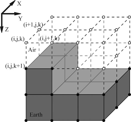
Discretization of a simple 3-D topology model for forward problem and adjoint problem in sensitivity calculation. The earth cells are marked with shaded colour. The filled circles and open circles show the earth nodes and air nodes, respectively. The solid lines are the earth edges, while the dashed lines denote the air edges. Note that the dotted edges are used both in the air and the earth in divergence operator.
Thus we define |${{{\bf G}}_A}$| as the gradient operator for air edges. For air edges which connect earth and air nodes, the Earth node is excluded from the gradient computation. Thus, gradients are computed on all interior air edges, under the assumption that the value of the scalar field on all boundary nodes (including the air–earth interface) are zero. For these air edges we set |$\lambda \equiv 1/{\sigma _{\rm {air}}}$|, so we effectively add |${{{\bf G}}_A}{{\bf De}} = 0$| to the original system of equations. For the earth edges, we add |${{{\bf \Lambda }}_E}{{{\bf G}}_E}{{\bf D\Sigma e}} = 0$|, where |${{{\bf G}}_E}$| is the gradient operator restricted to earth nodes, mapping to earth edges, and |${{{\bf \Lambda }}_E}$| represents scaling of earth edges.
If we put |${{\bf \Lambda }}$| before the gradient operator to apply the scaling factor on the nodes we simply add |${{\bf G\Lambda D\Sigma e}} = 0$| to the full system. Although scaling factors are vastly different between earth and air domains, there is no ambiguity about which domain a node belongs to, so using an average node conductivity leads to at least approximately correct scaling of the divergence correction.
Coefficient matrix structure
For the staggered grid, the standard second-order FD stencil for the curl–curl operator has 13 non-zero elements (nzs), while the stencil for the grad-div operator has 11. However, in the air (or anywhere where |$\sigma$| is constant and |$\lambda = 1/\sigma$|) many of these elements cancel out as the modified system of equations reduces to the vector Laplacian, with at most 7 non-zero elements per row. The change in sparsity pattern is illustrated in Fig. 2 for a toy problem (|$6 \times 6 \times 6$| grid with 2 air layers). The reduction in the number of non-zero matrix elements reduces computational time for the matrix-vector multiplies used by iterative solvers. More importantly, collapsing the null space of the curl operator leads to a substantial decrease in matrix condition number. For the toy problem of Fig. 2 the condition number drops from 1.45 × 10¹³ to 474.5. We can thus anticipate convergence of Krylov solvers for the modified system in fewer iterations. Further gains in efficiency can be expected from omission of the divergence correction iterations that solve (12) and (13).
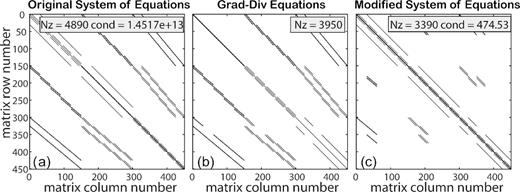
Sparsity pattern of a 6 by 6 by 6 (including 2 air layers) FD grid for: (a) original system of equations; (b) the grad-div equations; (c) the modified system of equations. Nz denotes the number of non-zero elements and cond is the condition number of the matrix. Note that only the matrix for interior edges (excluding boundaries) is shown. In this simple illustrative case there is some cancellation in the Earth, as the conductivity is homogeneous.
It is easily shown that |${{\bf VGD}}$| is also a symmetric matrix, but the diagonal matrices |${{\bf \Lambda }}$| and |${{\bf \Sigma }}$| break the symmetry. It is possible to modify the equations and still maintain symmetry—for example following the node based scaling approach, instead of adding |${{\bf VG\Lambda D\Sigma e}} = 0$| we can add |${{\bf \Sigma VG}}{{{\bf \Lambda }}^2}{{\bf D\Sigma e}} = 0$|, which still enforces the divergence-free conditions. However, our tests suggest that this alternative approach does not perform as well as a scheme based on (22), at least when we use a Krylov solver such as BiCGstab or QMR, which can handle non-symmetric systems. Partial symmetrization with |${{\bf V}}$| still does appear to accelerate convergence.
Non-zero current source
3 SENSITIVITY CALCULATIONS FOR INVERSE PROBLEMS
There are two (ultimately equivalent) ways to view computation of the sensitivity for the modified system. First, as the formal notation of (27) and (29) already suggests, we can view the solver as a ‘black box’ which solves the discretized equations for a specified input (i.e. forcing and boundary conditions). From this perspective, using the modified system of equations represents a regularization, or pre-conditioner, that improves efficiency of the solver, but does not ultimately change the forward problem. The inputs to any nominally equivalent solver, whether based on the original system matrix |${{\bf S}}$|(with divergence correction), or on the modified system |${{{\bf S}}_{\,\rm mod}}$|, should remain unchanged. Thus the matrices |${{\bf P}}$| and |${{{\bf L}}^T}$| still define the inputs to the (abstract black box) forward and adjoint solvers, respectively. However, as discussed at the end of the previous section, if inputs to the original forward problem are |${{\bf b}}$| (boundary data) and |${{\bf s}}$| (imposed source current; this will be |${{\bf P}}$| for the sensitivity calculation), the right-hand side for the modified system needs to be changed by addition of |${(i\omega \mu )^{ - 1}}{{\bf G\Lambda Ds}}$|. Similar modifications will be required for the right-hand side of the adjoint system, as discussed later.
Thus, (32) is ultimately solved for the same right-hand side, and the two approaches are equivalent. In ModEM |${{\bf L}}$|, |${{{\bf S}}^{ - 1}}$| and |${{\bf P}}$| are independent modules, so we find it more convenient to treat the forward solver as a black box which automatically adjusts the inputs before computing the solution. Then we can leave |${{\bf P}}$| unchanged, and use either the original, or the modified approach for the forward solver, without modifying other parts of the sensitivity calculation.
But |${{\bf D\Sigma }}{{{\bf e}}_0} \equiv 0$| so (35) reduces to the simpler expression (31). The same argument holds for other possible scaling factors which might have some dependence on model parameters.
Computations with the transposed Jacobian of (29) can be implemented with the same two approaches discussed for the forward problem. Although indirect arguments show that the same result will be obtained with either, this equivalence is apparently not readily established through simple closed-form expressions.
In contrast to the forward Jacobian calculation, it is not immediately obvious from the equations given that the black box and direct approaches should yield identical results for |${{{\bf J}}^T}$|, even within numerical precision. Different systems of equations are solved, with different right-hand side, and the results are multiplied by different matrices. However, we have shown that the same result for |${{\bf J}}$| are obtained with the two approaches, and the two different expressions for |${{{\bf J}}^T}$| are obtained formally by applying standard rules for matrix transpose. In Section 4, we demonstrate equivalence of the two approaches with computational examples. Within the modular ModEM code, we use the black box approach to computation of |${{{\bf J}}^T}$| or of matrix–vector products such as required for penalty functional gradients.
4 NUMERICAL RESULTS
As an initial comparison between forward solvers based on the modified and original systems of equations we consider one of the most widely used 3-D synthetic models: the COMMEMI 3D-2A model introduced by Zhdanov et al. (1997). The model includes two surface outcropping anomalies in a layered earth, with more details shown in fig. 5(b) of Zhdanov et al. (1997). The model is discretized into a 71 by 71 by 46 mesh (excluding air layers but including padding cells). MT forward responses are calculated at 6 periods from 0.01 to 1000 s. For these, and all other forward calculations we used the BiCGstab method, preconditioned with an incomplete LU decomposition. For calculations with the original system of equations, a divergence correction is performed every 40 BiCGstab iterations. All forward computations were done with a single process running on an Intel(R) Xeon E5 1.7 GHz. Iterations are set to terminate after the calculated relative residual is below 10−10. To simplify discussion, we use CC-DC (curl–curl equations followed by divergence correction) and CCGD (curl–curl equations modified by grad-div operator) respectively, to refer to the original and modified approaches.
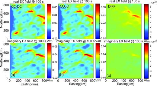
First, we compare forward solutions for the COMMEMI 3D-2 resistivity model using ModEM, with forward solvers based on CC-DC and CCGD methods. Fig. 3 compares the calculated surface electric field of XY mode at 100 s using the two approaches. It is quite clear that the surface electric fields computed with both approaches are nearly identical, with relative differences of order 10−7 or less. After all, we are still solving the same physical problem, just in a different way. It should also be noted that the most pronounced differences between the two solutions are located where the model conductivity is in harsh contrast. This is because contrasts in conductivity may result in abrupt changes in the magnitude of the |${{\bf G\Lambda D\Sigma e}}$| term in the neighbouring cells near the boundary, disrupting the relative weight of the curl–curl and grad-div terms.
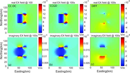
Comparison of the surface Ex field at the central part of COMMEMI 3D-2A model with XY polarization at a period of 100 s using (a) CC-DC approach and (b) CCGD approach. Panel (c) shows the electric field difference of (a) – (b).
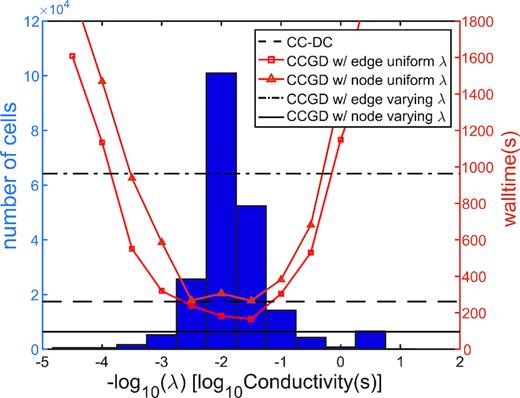
For the CCGD results shown in Fig. 3 the scaling factor was variable in space and applied at the nodes. Similar agreement with the CC-DC solution is obtained regardless of how the regularization term is scaled—that is implemented as |${{\bf G\Lambda D\Sigma e}}$| or |${{\bf \Lambda GD\Sigma e}}$|, with scale factors in the earth constant, or varying as |$\sigma _{Earth}^{ - 1}$|. On the other hand, performance is significantly affected by details of the scaling. This is illustrated in Fig. 4, where we plot the histogram of model conductivity values, together with wall-clock execution time for the COMMEMI 3D-2A modelling runs at a period of 100 s. If |$\lambda$| is taken as a constant in the earth, performance of course depends on the value used. For both edge and node cases run times are reduced, relative to CC-DC (indicate by the heavy dashed line) only for |$\lambda$| near the centre of the distribution of model conductivities. There is no clear advantage to either node or edge scaling, at least for this test model. The clear winner in terms of speed is spatially variable scaling applied to nodes. The same variable scaling applied to edges is remarkably slower, and in fact is considerably less efficient than the CC-DC approach.
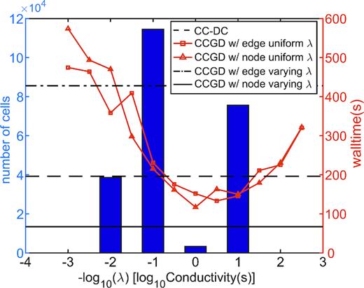
Distribution of conductivity values in COMMEMI 3D-2A forward model, with average computation time for XY mode forward calculation at 100 s. The dashed line denotes the calculation time using CC-DC approach. The solid line is the forward time for CCGD approach with spatially variable scaling factors λ, while the dot–dashed line gives the comparable result for variable edge scaling. The solid red lines with squares (triangles) denotes the computation time for different constant λ values for edge (node) scaling.
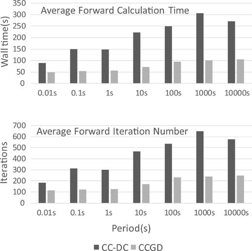
Fig. 5 provides a more detailed look at the relative performance of CC-DC and CCGD (variable node scaling), in terms of calculation time and iteration number for a range of periods. The computation time difference is negligible for shorter periods, where the divergence problem is less pronounced, and convergence with either system is fast. In fact, CCGD is slightly slower than CC-DC for the shortest period. As the period increases, the CCGD method gains a significant advantage, with wall times reduced up to 60 per cent of the CC-DC run time at 100 s (∼70.9 s versus 182 s). Note that the reduction of iteration count for the CCGD method is less significant than the reduction in wall time, as each iteration is faster due to the reduction in the number of non-zero elements in the system matrix. Furthermore, the dependence of computation time on period is weaker with the CCGD approach. For the CC-DC approach, time required by the slowest task (1000 s) is ∼5.14 times that of the fastest task (0.01 s). This ratio is only ∼1.93 for the CCGD counterparts. This can be advantageous for parallelized computations, as will be discussed in the inversion tests below.
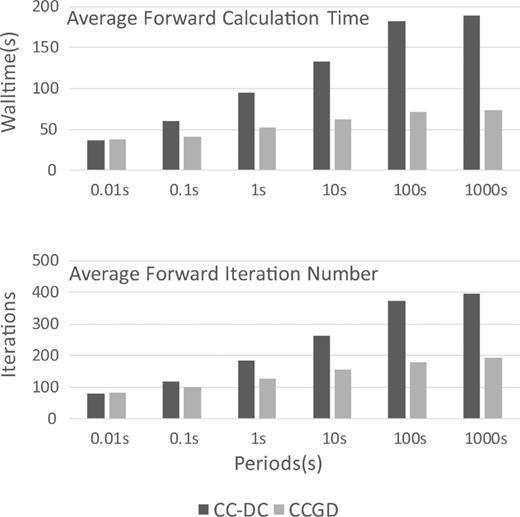
Comparison of run time (upper panel) and number of BiCGstab iterations required for convergence to a tolerance of 10−10 as a function of period for the COMMEMI 3D-2A model.
We also use the COMMEMI 3D-2A model to demonstrate the equivalence of the ‘black-box’ adjoint calculation [i.e. using (40) and (41)] to a more direct approach using the unmodified system. In Fig. 6 we show a section through the sensitivity for a single component of the impedance (|${Z_{xy}}$|) measured near the centre of the model (one column of |${{{\bf J}}^T}$|) computed with the adjoint solution as defined by (39). Relative differences from the sensitivity obtained using the original CC-DV approach are of order 10−5, and are largest on boundaries between blocks of different conductivity.
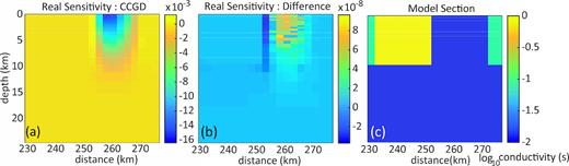
Comparison of different approaches to sensitivity calculation, for a single component of the impedance (Zxy) at a period of 100 s near the centre of the model domain. (a) shows section under site of real part of sensitivity computed with modified system of adjoint equations (CCGD), following (40) and (41). (b) shows difference from standard sensitivity calculation using unmodified system. Panel (c) shows corresponding section through COMMEMI 3D-2A model used for the calculations.
To evaluate the performance of the two approaches for more realistic MT forward and inverse calculations, we conducted a series of tests using the 3D inverse model of the Cascadia, USA region described by Patro & Egbert (2008). The model has a spatial dimension of 1460 by 1590 by 550 km (78 by 80 by 34, excluding air layers, but including padding cells) and includes the Pacific Ocean, an a priori constraint in the western part of the model domain. The resistivity model was originally obtained using the WSINV3DMT code (Siripunvaraporn et al.2005) to invert an initial subset of the USArray long-period MT data. This model is also included as a test example in the publicly available ModEM 3D MT inversion package (Kelbert et al.2014).
In the Cascadia forward test, forward responses of the Cascadia model for seven periods ranging from 0.01 to 10000s are calculated. Similar to the synthetic forward test, surface electric fields computed with both approaches for the Cascadia model are nearly identical, with relative differences of order 10−8 or less for the Ex field with XY mode at 100 s (Fig. 7).
Comparison of the surface Ex field of the central part of Cascadia model with XY polarization at a period of 100 s using (a) CC-DC approach and (b) CCGD approach. Panel (c) shows the electric field difference of a–b.
The different scaling approaches for the grad-div regularization term are also compared for the Cascadia inverse model in Fig. 8. Results are generally similar to those obtained with the simpler COMMEMI 3D-2A model: CCGD with spatially variable node (edge) scaling is much faster (slower) than CC-DC. Curiously, with fixed |$\lambda$| edge scaling works significantly better than node scaling. We give a more detailed comparison of performance for the CC-DC and CCGD (variable node scaling) approaches in Fig. 9. The CCGD approach has an advantage in both the convergence rate and calculation speed for almost all periods. For shorter periods, the computational speed advantage of the CCGD approach is less significant at ∼83 per cent (∼49 s versus 90 s at 0.01 s) with respect to the CC-DC method, while the difference increases to ∼200 per cent for longer period (∼101 s versus 307 s at 1000 s). As with the COMMEMI forward test results, the computation time is also more uniform for different periods with the CCGD approach. Time required for the slowest task (1000 s) is ∼3.42 times that of the fastest task (0.01 s) for the CC-DC approach. The ratio is only ∼2.15 with CCGD.
Distribution of conductivity values in the Cascadia inverse model, with average computation time for XY mode forward calculation at 100 s, overlain with comparison of efficiency for the 4 scaling approaches. Lines and symbols are as in Fig. 4.
Comparisons of (a) average calculation time and (b) average iteration number from forward calculations at different periods for the Cascadia model, using modified and original system of equations. The calculation time and iteration number are averaged from two polarizations. Note the longest computation time emerges at 1000s instead of the longest period.
To more fully assess performance of the modified approach in an inversion context, a series of tests are conducted using the Cascadia data as in Patro & Egbert (2008). The original starting model (80 × 78 × 34) with the ocean is used as we run a series of comparisons between the modified and original approach. Eight periods from the original study, ranging from ∼100 s to 7300 s are used in the inversions. The tolerances for forward and adjoint calculations are both set as 10−10 for this test.
Here 17 CPU cores (including one master to coordinate the parallelization) are used for the test inverse problem. All cores are identical to that used for the forward tests described above. A total of 185 and 198 iterations are taken before the inversions reach the desired misfit (RMS = 1.6) for the CC-DC and CCGD approaches, respectively. First, we compare the final models from both inversions. Fig. 10 demonstrates the horizontal sections of resistivity for the two models at 10, 30, and 70 km depths. It is obvious that the differences from the two inversion models are indistinguishable in the log10 resistivity domain. This shows that the CCGD approach is effectively equivalent to the traditional CC-DC approach.
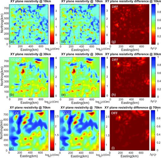
Comparison of horizontal resistivity of the Cascadia inversion model at 10, 30 and 70 km. (a–c) show the model calculated with CC-DC approach, (d–f) with CCGD approach and (g–i) shows the relative resistivity difference.
However, a small proportion of cells (∼1.5 per cent) show relative differences larger than 10 per cent (Figs 10h–j), even though the forward/adjoint calculation difference of the two approaches is around an order of 10−6 to 10−8. This is because a small difference in the forward/adjoint solutions will result in a larger error in the gradient, which directly determines the search step (and the model selected afterwards) in the model line search. The small differences at each step will obviously build up after ∼200 iterations, resulting in more significant differences in the final inverse solution. Also, given that the inverse solution conductivity can vary by orders of magnitude, slight shifts in position of a model feature in an area of large gradient can lead to localized patches with large relative differences. That said, the differences between the inverse solutions are not significant in practice, as for most of the cells the difference is smaller than 1 per cent.
Regarding the performance of the inversion, as the most time-consuming part of geophysical inversion calculations are essentially the forward and adjoint (sensitivity) calculations, the efficiency of the inversion computations should be similarly improved as in the forward cases. The real-world performance difference in a coarse-grain (period-wise) parallelization scheme (as used in ModEM) often comes from the forward calculation for the longest periods. This is because such parallel schemes distribute each period/polarization to one processer, so the slowest forward problems will determine the wall-clock time for the entire calculation. As shown in the forward tests, the CCGD approach leads to a more balanced workload among different periods/polarizations. Therefore, it is naturally more efficient in such schemes.
Fig. 11 compares the overall time required for inversion of the Cascadia data set using different forward solvers. It is clear that the CCGD approach also drastically improves the computational efficiency of the inversion, which is more than 160 per cent faster than the traditional CC-DC method (with wall time of ∼677 min versus 1791 min) in term of overall computational speed. Both forward and adjoint calculations are similarly accelerated. Note that the FWD calculations took roughly twice as much time as adjoint calculations in our inversion test. This is because in ModEM, one NLCG iteration normally requires two forward calculations and only one adjoint calculation (see Kelbert et al.2014 for details). The ‘other’ time consumption (I/O, MPI communications, etc.) is similar (∼4 min) for both approaches as both use the same basic modules in ModEM.
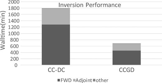
Comparison of computation time of Cascadia inversion with forward calculation based on CCGD and CC-DC methods.
5 DISCUSSION AND CONCLUSIONS
It is clear from our results that success with the CCGD approach depends critically on the scaling of the GD term. In a region of constant conductivity (e.g. in the air, where a small constant |${\sigma _{air}}$| is used) we expect |$\lambda = {\sigma ^{ - 1}}$| to be optimal, as this will reduce the curl–curl operator to the (vector) Laplacian, and essential eliminate the (near) null space of the quasi-static EM operator. However, this simplification will not hold exactly for even the simplest heterogeneous models, and it is probably better to view the scaling as providing a relative weighting of two constraints on the solution—that is the curl–curl equation, and the divergence-free condition |$\nabla \cdot \sigma E = 0$|. Weighting the second constraint by |$\lambda \approx {\sigma ^{ - 1}}$| should enforce both constraints at a similar level in the iterative solution schemes used. Clearly, very different weights must be used within air and earth domains, which typically differ in conductivity by up to 10 orders of magnitude. If, as may often be common in practical (regularized) inversions, conductivities cluster around a central value, the inverse of this mean (perhaps better, median) conductivity might provide a reasonable scalar weight within the Earth domain. However, even for something simple like the COMMEMI model (which has a bimodal distribution of conductivities) there may be no single good scaling factor within the Earth, so we have been motivated to consider spatially varying weights. For all examples we have tested we find that a spatially variable weighting of the divergence-free condition provides the best performance.
This approach is also not without problems, as the appropriate scaling is ambiguous near blocks of different conductivity, or where gradients are sharp. And note that even a smooth regularized inversion may contain discontinuities in conductivity, especially if constraints (such as an ocean domain) are included. As we discussed specifically in the context of the air-earth interface this ambiguity in scaling is especially clear when we apply the (spatially variable) scaling factor on grid edges, after computing gradients. Each grid node corresponds to one constraint on current divergence |$\nabla \cdot \sigma E = 0$|, a balance between terms that must be comparable. Probably the best (but still imperfect) scaling for this constraint should be some average of the conductivities surrounding the node. Near a sharp gradient in conductivity the gradient of this divergence will couple nodes which should properly have greatly different scaling. We hypothesize that this may explain the poor performance of variable scaling applied to edges, even while this variable scale approach seems to be the best choice when applied on the nodes. Further study of the fundamental differences observed between scaling approaches is warranted.
Calculation of the gradient of the data misfit sum of squares during an inversion search (e.g. with NLCG) requires computation of the sensitivity matrix-residual product |${{{\bf J}}^T}{{\bf r}} = {{{\bf P}}^T}{{{\bf S}}^{ - T}}{{{\bf L}}^T}{{\bf r}}$|. We have shown that when we use the modified coefficient matrix |${{{\bf S}}_{\,\rm mod}}$| there are two distinct approaches to this calculation. The first is based on modification of the right-hand side for the adjoint solver [i.e. modify |${{{\bf L}}^T}{{\bf r}}$|; see (40) and (41)] and then multiply the resulting adjoint solution by |${{{\bf P}}^T}$| computed for the original coefficient matrix. The second, perhaps more direct, approach is to solve |${{\bf S}}_{\,\rm mod\,}^T{{\bf x}} = {{{\bf L}}^T}{{\bf r}}$| (without modifying the right-hand side of the modified adjoint system) and then completing the computation as |${{{\bf J}}^T}{{\bf r}} = {{\bf P}}_{\,\rm mod\,}^T{{\bf x}}$|, using a modification of |${{{\bf P}}^T}$| appropriate for the modified coefficient matrix. The argument for equivalence of these two approaches is rather indirect, but mathematically sound. Direct calculation demonstrates that equivalent results for sensitivities are indeed obtained with either approach.
While in the above study our efforts are focused on regularization of an electrical field formation of the second order Maxwell eq. (1), an equivalent regularization term can be applied to the magnetic formulation (2). In this case the conservation condition becomes |$\nabla \cdot B = 0$| for the whole model domain, so the regularization term becomes |$\nabla (\nabla \cdot H) = 0$|, by applying the gradient (and dividing by an assumed constant magnetic susceptibility). As resistivity now appears in the first term on the left-hand side of (2), it is natural to scale the regularization term with a factor of |$\lambda = \rho = {\sigma ^{ - 1}}$|, for dimensional consistency between the curl–curl and grad-div terms. This is the approach taken by Weaver et al. (1999). Note that the regularization term (23) in the actual implementation would become |${{\bf VG\Lambda Dh}} = 0$|, which still retains symmetry. Thus, the regularization approach may be even more attractive for the magnetic field formation, given that a symmetric system is often easier to solve.
We have presented a divergence-free solution approach for time-harmonic Maxwell equations in frequency domain geophysical EM methods. The curl–curl equation is modified, and effectively regularized, by addition of a scaled grad-div operator to simultaneously enforce the divergence gauge condition and the usual curl–curl equation. This approach has been implemented with total electrical field formulation within the ModEM 3-D inversion code (Kelbert et al.2014) and compared with the more standard approach (in EM geophysics) where the divergence correction is performed every few Krylov iterations. Comparison on synthetic and real-world problems shows that the new approach significantly improves computational efficiency in both forward and inversion calculations. The improvements on cases we have tested so far are substantial enough to suggest that the new approach will have a very significant impact for practical applications of 3-D inversion. Further research on improvement in solver efficiency are warranted. In particular, the modified system of equations we solve here is much more diagonally dominant, closely approximating a Poisson equation. In contrast to the original curl–curl equations, systems of this sort can often be solved very efficiently with an algebraic multigrid approach. Exploring this possibility is an obvious next step.
We also believe this approach can be extended to other numerical methods (e.g. finite volume or finite element methods), since the foundation of this divergence-free approach is built on the strong form. With the added regularization term, the null space of the curl operator should be similarly deflated, with the condition number of the discrete system improved regardless of the numerical method used. Of course, the actual performance of this approach in other methods cannot be guaranteed without tests. Assembly of the regularized system would involve the construction of discrete divergence and gradient operators, which should be trivial for staggered grid finite volume or Lagrange finite element methods. However, these operators may not be readily available in some methods, requiring additional effort. For example, in FEM with Nedelec curl-conforming elements, the gradient and divergence operators have to be built in an auxiliary H(1) space, with the curl operators in H(curl) space, as demonstrated in Hiptmair & Xu (2007) method.
ACKNOWLEDGEMENTS
Discussions with Randall Mackie provided the original motivation for this work and helped clarify several issues. The authors thank Dr Alexander Grayver and an anonymous referee for comments that improved the manuscript. Funding for H.D. was provided by NSFC grant 41504062 and 863 program 2014AA06A603. Partial support for GDE was provided by NSF grant EAR1225496.
REFERENCES
APPENDIX: SOME TECHNICAL DETAILS
If air conductivity is zero, the inverse coefficient matrix |${{{\bf S}}^{ - 1}}$| used in (27) is not defined, and the formal manipulation used to derive the adjoint expression (29) might be questioned. Furthermore, for the modified system (which actually should be non-singular even without a non-zero air conductivity) we argued that for solving the adjoint problem the source term, scaled by the inverse of grid volume weights, should vanish in the air. The source for the adjoint problem of (29), which is derived from the linearized data functional |${{{\bf L}}^T}$|, can in fact extend into the air (e.g. because magnetic fields need to be interpolated to the air-earth interface). It is not immediately clear that |${{{\bf V}}^{ - 1}}{{{\bf L}}^T}$| will be divergence free in the air. We thus explicitly omit the component of |${{\bf D}}{{{\bf V}}^{ - 1}}{{{\bf L}}^T}$| that lies in the air domain when modifying the RIGHT-HAND SIDE of (36), but make no comparable adjustment to |${{\bf L}}$| in the direct sensitivity calculation of (27), or in the original source term |${{\bf s}} = {{{\bf L}}^T}$| in (36). Here we demonstrate more formally the consistency of this approach.
Any edge vector can be uniquely represented as a sum of solenoidal and irrotational components |${{\bf x}} = {{{\bf x}}_C} + {{{\bf x}}_G}$|, which from (A2) will be orthogonal with respect to the edge-volume-weighted inner product. Of course we have |${{\bf D}}{{{\bf x}}_C} = 0$| and |${{\bf C}}{{{\bf x}}_G} = 0$|. All of this holds if we restrict all vectors, scalars, and operators to the air domain, following the conventions of Fig. 1 and associated discussion.
Thus, the irrotational component of the (scaled) data functional (in the air) makes no contribution to the forward sensitivity calculation of (27); omitting this from the source for the adjoint calculation is thus consistent with the requirement that |${{\bf e}}$| be divergence-free in the air. Note that the full data functional vector |${{{\bf L}}^T}$| (including any components in the air) should be included in the original source term [i.e. |${{\bf s}}$| in (36)], but the correction |${{\bf D}}{{{\bf V}}^{ - 1}}{{\bf \Lambda }}{{{\bf L}}^T}$| should be limited to Earth nodes.
