


SUMMARY
We use 1 month of continuous seismic waveforms from a very dense seismic network to image with unprecedented resolution the shallow damage structure of the San Jacinto fault zone across the Clark fault strand. After calculating noise correlations, high apparent velocity arrivals coming from below the array are removed using a frequency–wavenumber filter. This is followed by a double-beamforming analysis on multiple pairs of subarrays to extract phase and group velocity information across the study area. The phase and group velocity dispersion curves are regionalized into phase and group velocity maps at different frequencies, and these maps are inverted using a neighbourhood algorithm to build a 3-D shear wave velocity model around the Clark fault down to ∼500 m depth. The model reveals strong lateral variations across the fault strike with pronounced low-velocity zones corresponding to a local sedimentary basin and a fault zone trapping structure. The results complement previous earthquake- and seismic noise-based imaging of the fault zone at greater depth and clarify properties of structural features near the surface.
1 INTRODUCTION
The properties and structures of the heavily damaged material in the top few hundred metres of the crust are understood only in general terms due to the lack of resolution of standard imaging techniques and strong local heterogeneities at shallow depths. Classic local earthquake tomography is best suited below 2–3 km, standard noise-based imaging with frequencies up to 1 Hz have resolution below 500 m, while small active seismic sources resolve mostly the first tens of metres of the subsurface. Having a better understanding of crustal structures and processes at this depth range is crucial, especially near fault zones, because of their great influence on observed seismic motion, crustal hydrology, reliability of underground facilities and numerous other applications. The low normal stress at shallow depth renders the subsurface material highly susceptible to failure and strongly attenuative, masking details of deeper structures and processes. Deriving detailed images of the very shallow crust can allow seismic velocity models to be developed essentially up to the surface, where they may be combined with information obtained from geological mapping and boreholes. The San Jacinto fault zone (SJFZ) is the most seismically active structure of the plate–boundary between the Pacific and North America plates in southern California, with a slip rate of about 10–15 mm yr−1 (e.g. McGill et al. 2015; Rockwell et al. 2015). It runs parallel to the San Andreas fault to the NE and the Elsinore fault to the SW and is thought to have a recurrence rate of major earthquake (MW > 7.0) of about 185–254 yr (Rockwell et al. 2015). The last earthquake which may have ruptured the total 230 km length of the fault likely occurred on 1800 November 22 (Rockwell et al. 2015), indicating that the SJFZ presents a serious seismic hazard for the region in the near future.
The Trifurcation area of the SJFZ, the region where the Clark fault is joined by the Bulk Ridge fault and the Coyote Creek fault (Fig. 1a), has ongoing small to moderate earthquake activity and generates >10 per cent of the recent seismicity in southern California (e.g. Ross et al. 2017). This complex faulting geometry is in contrast to the simpler section of the Clark fault to the NW, referred to as the Anza seismic gap (Sanders & Kanamori 1984), with a lack of microseismicity and potential source of MW6.5 earthquakes. Previous imaging studies in the area used local earthquake tomography and ambient noise with frequencies up to 1 Hz to clarify properties of the fault zone at seismogenic depth (Scott et al. 1994; Allam & Ben-Zion 2012; Allam et al. 2014; Zigone et al. 2015). However, the properties in the top 500 m of the crust remained unresolved and are targeted in this work.
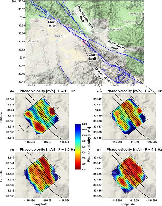
Phase velocity maps at four different frequencies obtained from DBF (Roux et al. 2016) on top of the local topography (Map data, Google, 2018). The black dots show the station configuration, the colour dots the local phase velocity. The thick black line indicates the surface trace of the Clark fault. The top panel (a) shows the general tectonic context of the studied area (red square) on a topography map of the Trifurcation area of the SJFZ (Map data, Google, 2018). The blue lines are the regional fault traces with their names. (b) 1.5 Hz, (c) 2.0 Hz, (d) 3.0 Hz and (e) 4.5 Hz.
Damage fault zone structures have strong heterogeneities of seismic properties including lateral interfaces that produce additional phases and complex wavefield (e.g. Ben-Zion & Aki 1990; Hillers et al. 2014). The intense seismicity and complex wavefield in the study area require using special techniques to suppress impulsive earthquake signals and extract Rayleigh surface waves from the remaining ambient seismic noise data that can be used for tomographic imaging (Shapiro et al. 2005; Roux 2009; Roux et al. 2011). This challenging task is accomplished using the pre-processing procedure and iterative double-beamforming (DBF) phase extraction technique of Roux et al. (2016). The obtained phase and group velocities of Rayleigh waves are inverted for shear wave velocities in the shallow crust with a neighbourhood algorithm (Sambridge 1999). The derived 3-D shallow structure of the fault zone closes an important observational gap between previous seismic imaging studies and geological mapping in the area.
2 AMBIENT NOISE TOMOGRAPHY FROM A DENSE SEISMIC ARRAY
Following previous work on high-resolution imaging from ambient noise correlations of dense array data (e.g. Lin et al. 2013; Mordret et al. 2013a), we produce here local images of the shear wave velocity at the SJFZ. We first describe briefly the data and main methodological steps needed to construct accurate dispersion curves of Rayleigh waves from the noise correlations in the complex study area following Roux et al. (2016). The employed data were obtained by a dense rectangular array with 1108 (10 Hz) vertical geophones and linear dimensions of about 650 × 700 m2 (Fig. 1). The array was centred on the damage structure of the Clark fault in the Trifurcation area of the SJFZ, southeast of Anza (Fig. 1), and recorded waveforms continuously at 500 Hz for about 1 month in 2014 (Ben-Zion et al. 2015). Each row along the fault-normal (x) direction had 55 sensors with an intersensor distance of 10 m, and the nominal separation between the rows in the along-strike (y) direction was 30 m. Each element of the seismic array provided continuous GPS-synchronized records.
2.1 Reliable extraction of Rayleigh waves information in fault zone region
Despite the incoherent noise generated by the ocean and by nearby sources (e.g. wind or human related), recent analyses suggested that numerous impulsive signals recorded by the array are generated by sources below the surface (Ben-Zion et al. 2015). Their apparent random temporal occurrence, without clear diurnal pattern, suggests that they do not have a thermal or man-made origin. In addition to many distinguishable microseismic events (Meng & Ben-Zion 2018), the waveforms contain large sets of long bursts that are typically grouped with the ambient seismic noise extending down to 1 Hz. To account for the presence of impulsive spikes in the waveforms, one-bit noise correlation is applied to 1 d long recording windows between all sensor pairs of the network. The averaged 1 d cross-correlations show a strong contribution around time t = 0, which suggests that most of the coherent signals are coming from below the array with very high apparent velocities, consistent with the presence of body waves (Roux et al. 2016). Because of the complexity of the ambient wavefield, all the processing (from raw data to velocity measurements) is done in narrow frequency band (about an octave). This increases significantly the quality of the measurement (for instance, one-bit normalization becomes quite robust) as well as the computational effort.
Figs 1 and 2 show Rayleigh wave phase and group velocity maps obtained at 1.5, 2, 3 and 4 Hz from the phase slowness and traveltime inversion on a regular horizontal grid with steps of 15 m. The tomography inversion starts from a homogeneous initial model, assuming straight rays as propagation paths and an a priori error covariance matrix that decreases exponentially with distances over 50 m (Roux et al. 2016). For the group velocity map, the inversion is performed with a random subsample of all the measurements and repeated 1000 times. The average results of these 1000 inversions give the final group velocity maps and the standard deviation gives their uncertainties. We use this procedure to reduce the computational burden of inverting more than 400 000 dispersion curves at once. This also allows us to obtain robust statistical estimate of the group velocity uncertainties. At each frequency, the phase or group velocity inversions produce a residual variance reduction of ∼95 per cent relative to the phase slowness and ∼98 per cent relative to the traveltimes of the homogeneous model. The topography has a maximum of 50 m elevation difference on the array and is not taken into account in the inversions (as suggested in Pilz et al. 2013). The smallest wavelength that we are measuring is on the order of 60–65 m and may only affect our estimation of the group velocity for which the distance between the subarrays is used to compute the velocity. Despite this approximation, the correlation between the group velocity maps and the topography is not obvious.
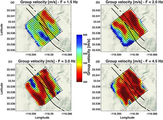
Group velocity maps at four different frequencies obtained from DBF (Roux et al. 2016) on top of the local topography (Map data, Google, 2018). The black dots show the station configuration, the colour dots the local group velocity. The thick black line indicates the surface trace of the fault. (a) 1.5 Hz, (b) 2.0 Hz, (c) 3.0 Hz and (d) 4.5 Hz.
Note that with this approach phase velocity is assumed to accumulate over propagation distance, similarly to group velocity, following the Fermat principle. However, phase velocity should instead be considered as a local value below each 25-element array used to perform the DBF. This requires extracting two phase slowness instead of one following the procedure described in Roux et al. (2016; see their eqs 2– 4 for details) at the price of a significantly larger computation effort. This assumption is valid if the propagation medium is not too complex, that is, when the two subarrays are close to each other. At longer distance, multipathing is stronger and the phase velocity estimations are less reliable. As for eikonal tomography (Lin et al. 2009; Mordret et al. 2013c), the phase slowness extracted from each subarray pair through DBF can be locally averaged to produce equivalent phase velocity maps (Fig. 1) and used to estimate the uncertainties.
The tomography results show strong lateral variations across the fault traces. The red low-velocity zone near the right fault line observed at lower frequencies in the phase velocity maps (Figs 1 a and b) corresponds to the fault zone trapping structure identified in Ben-Zion et al. (2015) and Qin et al. (2018) using active experiment data and earthquake waveforms. The results for increasing frequencies have complex features that correspond progressively to shallower depth. Note that phase velocity maps seem to be at first sight more interpretable than group velocity maps as suggested from their relative sensitivity kernel analysis (Supporting Information Fig. S1). Phase velocity sensitivity always exhibits a positive kernel with one main maximum implying that a shear wave velocity anomaly at depth will be positively correlated with the phase velocity at the frequency sensitive to this depth. On the other hand, group velocity kernels exhibit two main extrema: one positive and one negative at different depths. Therefore, at a single frequency, group velocity maps show the weighted average of shear velocity structures that are positively correlated at one depth with shear velocity structures that are negatively correlated at another depth. This makes it difficult to interpret the resulting group velocity values. Another consequence of the group velocity kernel shape is that a single positive shear wave velocity anomaly at a specific depth may be seen as positive or negative group velocity anomalies depending on frequency. The wavelength range of the Rayleigh waves used here suggests that the imaging results characterize the top 50 m to 400–500 m of the crust.
2.2 Inversion with a neighbourhood algorithm
The full set of phase and group velocity maps provides local dispersion curves at each cell of the map. These local dispersion curves for phase and group velocities are jointly inverted to obtain local 1-D profiles of Vs versus depth. The ensemble of every best local 1-D model constitutes the final 3-D Vs model.
Inverted parameters and their ranges.
| Parameter | Unit | Min | Max |
|---|---|---|---|
| V0 | m s−1 | 100 | 600 |
| α | 0.15 | 0.3 | |
| β | 2 | 5 | |
| A1 | m s−1 | −500 | 1000 |
| A2 | m s−1 | −500 | 1000 |
| dn | m | 400 | 1000 |
| Vp/|$V_{{\text {s}}_{0}}$| | 1.5 | 2.5 | |
| Vp/|$V_{{\text {s}}_{n}}$| | 1.6 | 2.0 |
| Parameter | Unit | Min | Max |
|---|---|---|---|
| V0 | m s−1 | 100 | 600 |
| α | 0.15 | 0.3 | |
| β | 2 | 5 | |
| A1 | m s−1 | −500 | 1000 |
| A2 | m s−1 | −500 | 1000 |
| dn | m | 400 | 1000 |
| Vp/|$V_{{\text {s}}_{0}}$| | 1.5 | 2.5 | |
| Vp/|$V_{{\text {s}}_{n}}$| | 1.6 | 2.0 |
We sample a total of 24 000 models at each geographical point of our grid. The initial random sampling is done with 10 001 models; then the Voronoï cells around the best 1000 models are resampled with 2 models and this process is iterated seven times (Mordret et al. 2014). The final model is the average of the 2000 best models (with the lowest misfits). The uncertainties of the velocity model are estimated by the standard deviation of the posterior distribution of the best 2000 models. Figs 3(a) and (b) show two examples of local inversions at two different positions on the grid (Fig. 3c). The colours show the misfit, the grey curves are the best model and its associated dispersion curves, and the black bars are the measured dispersion curves. During each inversion, we used a misfit defined by Mordret et al. (2014) as a ratio of two surface areas, Misfit = dS/S, with S being the integral surface area of the measured dispersion curve and its error bars and dS the integral surface area of the synthetic dispersion curve outside of S. With this definition, the misfit presents a wider minimum area and permits to retain dispersion curves as long as they fit the data within their error bars.
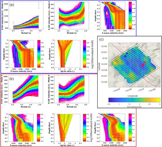
Local depth inversion at two locations in the model: the top-left panel shows the phase velocity dispersion curve fit, the top-middle panel shows the group velocity dispersion curve fit and the top-right (bottom right for point B) panel shows the sampled Vs models. The bottom-left panel shows the sampled Vp models and the bottom-middle panel the Vp/Vs ratios. The inverted data are in black with the error bars; the best model and the dispersion curves associated with the best model are in grey. The colour of the modelled dispersion curves and their associated models indicate their misfit value. (a) Inversion of a point on top of the main Clark fault trace. (b) Inversion of a point east of the fault. (c) Map of the best model misfit on top of the local topography (Map data, Google, 2018). The fault traces are shown by the red lines. The seismic array is shown by the black dots and the locations of the points inverted in panels (a) and (b) are indicated by the blue and red circles, respectively.
The misfit map has strong lateral variations (Fig. 3c) that mostly reflect difficulties to fit some local phase dispersion curves (Fig. 3a). For some frequencies, the phase velocity has large uncertainties and does not seem to be consistent with velocities at neighbouring frequencies. This might indicate discontinuities within cell’s phase dispersion curves due to lateral heterogeneities, contamination by higher order modes, body waves or local anthropogenic noise (southwest of the fault). Local measurements of phase velocities across the fault reveal strong changes on short distances associated with low-velocity damaged zones (see fig. 12 in Roux et al. 2016). Future work will focus on local extraction of phase slowness as discussed in Section 2.1 and its interpretation through both local anisotropy and damage.
The group velocities are comparatively more robust, essentially because of the lack of phase ambiguity measurements but they also exhibit discontinuities to some extent. Again, contamination by higher modes, body waves or sensor coupling may be at the origin of these jumps. To assess the benefit of jointly inverting phase velocities with group velocities, we performed an inversion of the group velocity alone (Supporting Information Fig. S2). For the same two points as in Fig. 3 we achieve much smaller misfits. However, it clearly appears that the dispersion curves are overfitted and do not correspond to physically and geologically reasonable velocity models. The addition of phase velocity dispersion curves in the inversion, despite their larger uncertainties, helps to diminish the non-uniqueness of the solution (e.g. Shapiro & Ritzwoller 2002). In conclusion, the constraints brought by the phase velocities, although weak, facilitate the rejection of highly unreasonable models and strengthen the robustness of the results.
3 INVERSION RESULTS
The derived 3-D model shows lateral velocity variations of about 20–30 per cent at all depths (Figs 4a, b and 5a, b) with several structures parallel to the fault strike (Figs 4 a and b). The velocity uncertainties are correlated with the velocity structures with higher uncertainties for higher velocities (Figs 4 c and d). They also tend to increase with depth, showing uncertainties smaller than 100 m s−1 above 100 m depth and up to 250–300 m s−1 below this depth. This reflects the extra constraint from Vp and density in the near surface (Supporting Information Fig. S1). The inversion results confirm that the assumed initial average velocity profile following a modified power law is a good model for the very shallow velocity structure (Fig. 5c). The two surface fault traces (black dashed lines in Figs 5 a and b) clearly delineates a low-velocity zone encompassed by higher velocities to the SW and slightly lower velocities to the NE (Fig. 6). This sharp lateral contrast even more clearly present in the depth variations of the isovelocity contour at Vs = 850 m s−1 (Fig. 7), which is a proxy for the transition between the loose near surface sediments and the more compact rocks at depth. A trough beneath the surface fault traces is consistent with damaged rocks producing deeper low-velocity material than directly to the west. This low-velocity zone corresponds to the local seismic trapping structure observed by Ben-Zion et al. (2015) and Qin et al. (2018).
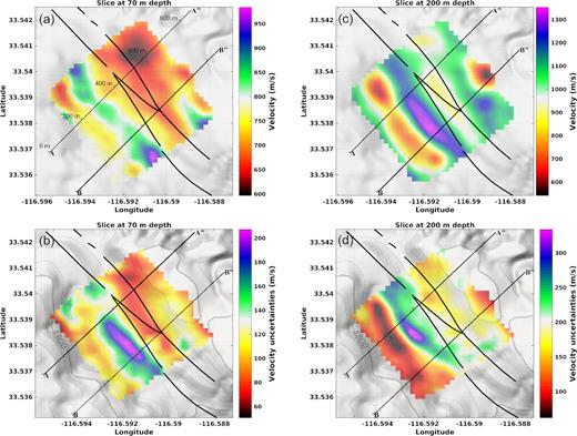
Horizontal slices in the 3-D velocity model at 70 m depth (a) and 200 m depth (b) on top of the local topography (Map data, Google, 2018). Horizontal slices in the 3-D uncertainty model at 70 m depth (a) and 200 m depth (b) on top of the local topography. The main Clark fault trace is shown with thick black curves. The locations of the vertical profiles shown in Fig. 5 are displayed with the thin black lines and graduated every 200 m.
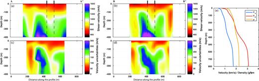
Vertical slices in the 3-D velocity model, the bold black lines and the dashed lines show the surface traces of the faults and their vertical prolongation at depth, respectively. (a) Profile A–A”, (b) Profile B–B”. Vertical slices in the 3-D uncertainty model. (c) Profile A–A”, (d) Profile B–B”. The locations of the profiles are shown in Fig. 4. (e) Average Vp, Vs and density models.
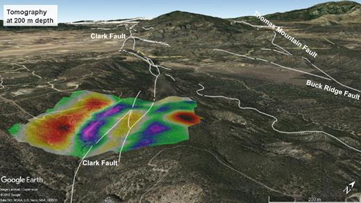
The velocity model in the tectonic context: shear wave velocity model at 200 m depth draped on the local topography. The fault traces are shown with white lines. The orange/red areas indicate slower than average velocity zones. The green/blue areas indicate faster than average velocity zones.
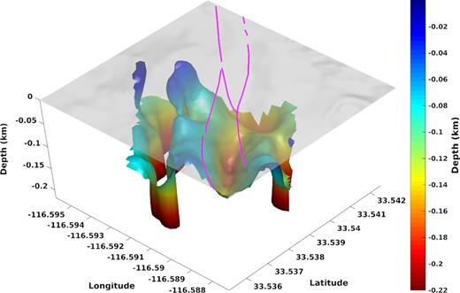
Isovelocity contour at Vs = 850 m s−1 showing the base of the compacting sediments. The fault trace is underlain by a trough of low-velocity material restricted by ridges of higher velocity material in the southwest and northeast. The fault trace is shown with the magenta lines at the surface on top of shaded digital elevation model. The isovelocity surface and the digital elevation model do not have the same vertical exaggeration.
Given the final misfit in the most southwestern part of the model (Fig. 3c) and the large uncertainties associated with the estimations of the depth of the half-space (Fig. 3a), the deep trough in the SW of Fig. 7, at the location of a small sedimentary basin, should be interpreted with caution. Overall, the robust qualitative features of the model (and the ones explaining most of the variance in the data) are the power-law increase of the velocity with depth within the near surface sediments, consistent with compaction (e.g. Baldwin & Butler 1985; Bachrach et al. 2000), the lateral variations across the fault traces and the depth variations of the base of the compacting layer. In such a complex environment, however, this simple model might be quantitatively biased by the simplifications we make during the modelling. Assuming a linear gradient-like Vp/Vs ratio in the near surface is one of them. Supporting Information Fig. S3 shows horizontal and vertical slices through the 3-D Vp/Vs model. We can observe lateral variations that seem to be parallel to the fault strike and most of the model exhibit an increase of Vp/Vs ratio with depth. The scattering of the best models in Fig. 3 suggests that this increase may not be a robust feature of our inversion. Among other simplifications, we do not take into account the attenuation and the anisotropy while inverting for the velocity model. These parameters may not be negligible in the centre and heavily damaged part of this fault zone as highlighted by previous studies (Ben-Zion et al. 2015; Hillers et al. 2016). However, the pre- and post-processing used to compute the noise correlations and extract the Rayleigh waves strongly affect the signal amplitudes, making the extraction of attenuation information difficult. Analysing the noise data with a procedure of the type developed by Liu et al. (2015) can provide information on the attenuation coefficients. Regarding anisotropy the vertical component sensors are used in this study can provide information only on the azimuthal anisotropy of the Rayleigh waves. Resolving radial anisotropy (e.g. Tomar et al. 2016) expressing the difference in propagation speed between horizontally and vertically polarized waves requires three-component data. An analysis of azimuthal anisotropy through an eikonal tomography approach (Mordret et al. 2013b; Zigone et al. 2015) will be the subject of future work.
4 DISCUSSION AND CONCLUSIONS
Building on the methodological work of Roux et al. (2016), we image with an unprecedented resolution the shallow damage structure of the SJFZ at the site of the dense seismic deployment (Fig. 1). The complex environment, both in terms of structure and variety of seismic signals, requires the use of innovative techniques to extract the surface wave information needed to perform the tomography. The derived 3-D shear wave velocity model for the top 500 m of the crust complements information obtained with more standard earthquake- and noise-based imaging techniques on the deeper structure of the fault zone, and allows direct comparisons with geological observations made at the surface (Wade et al. 2017).
A previous attempt to image fault zone structure with ocean-induced seismic noise was performed on the San Andreas fault in Parkfield at lower frequency (<0.35 Hz) and at a larger scale from 30 stations in a 10 km x 10 km area (Roux et al. 2011). A 1.3 km wide steep dipping was imaged from less than 400 local dispersion curves for Love waves. Joint inversion of body wave arrival times and these surface wave dispersion curves were applied to further constrain a “U-shaped” feature of the 3-D seismic structure around San Andreas Fault Observatory at Depth. (SAFOD) (Zhang et al. 2014). It seems that a similar feature is observed in Fig. 7, though at a much smaller scale. In our study area the U-shaped feature is produced by a narrow low-velocity zone delimited by the surface fault traces trapped between two higher velocity ridges to the SW and the NE(Figs 6–7). Qin et al. (2018) concluded based on earthquake waveforms that the SW fault trace represents the main seismogenic fault separating two different crustal blocks at depth. The asymmetry between the high velocities to the SW and the lower velocities to the NE tends to confirm this interpretation. Theoretical and numerical results indicate that earthquakes on a bimaterial interface tend to have preferred rupture direction (Ben-Zion 2001, and references therein) and produce asymmetric shallow damage structure on the less compliant side of the fault at depth (e.g. Ben-Zion & Shi 2005; Xu & Ben-Zion 2017). In the study area, regional tomographic images have shown that the NE side of the main Clark fault is faster than the SW block at seismogenic depth (Scott et al. 1994; Allam & Ben-Zion 2012; Allam et al. 2014; Zigone et al. 2015). Therefore, it is expected that rock damage be more pronounced on the NE side of the fault in the near surface, generating a shallow velocity contrast inversion between the local scale and the regional scale structures. This is confirmed by the local contrast of seismic velocities across the main Clark fault imaged in this study (Figs 4 and 6) and is consistent with local geological mapping (Wade et al. 2017) and agrees with the general NW directivity of earthquake ruptures in the area.
The results of this work mainly provide isotropic shear wave velocities of the subsurface structure. Future studies can improve the seismological characterization of the study area by deriving information on the compressional wave velocity, attenuation coefficients and anisotropy. Research on some of these topics is currently under way. Fang et al. (2016) derived a 3-D velocity model for the plate–boundary region around the SJFZ with a nominal resolution of about 3 km from joint inversion of surface wave and body wave measurements. Similar analysis can be performed for the site of the dense deployment using our surface wave results and the collection of active shots recorded on the dense seismic grid (Ben-Zion et al. 2015). Following Nakata et al. (2015), refracted and/or reflected body wave arrivals could also be extracted directly from ambient noise correlations from the microseismic activity at depth in the fault zone. The lateral spatial resolution in the sampled area should be lower than 50 m for a detailed 3-D image down to 500 m at depth.
The site of the dense deployment used in this work is becoming a natural laboratory for collecting and correlating different types of geological data (detailed mapping, laboratory characterization of rock samples) and geophysical results (seismic, geodetic, electrical resistivity, GPR). The 3-D velocity model developed in this paper for the very shallow crust provides a fundamental component for the effort to compare and correlate different fault zone data sets. It will also help to better constrain results on temporal changes of seismic velocities from various sources, and understand properties of earthquake ruptures in the area.
SUPPORTING INFORMATION
Figure S1. (Top panels) Phase and (bottom panels) group velocity depth sensitivity kernels computed at three different periods in the average velocity model for Vs, Vp and density.
Figure S2. Local depth inversion at the two locations (point A, top panel in blue and point B, bottom panel in red) in the model shown in Fig. 3, using only the group velocity dispersion curves. The inverted data are in black with the error bars; the best model and the dispersion curves associated with the best model are in grey and the colour of the modelled dispersion curves and their associated models indicate their misfit value. Note the strong non-uniqueness of the solutions with two families of models competing.
Figure S3. (Top panels) Horizontal slices in the 3-D Vp/Vs ratio model at 70 and 200 m depth. (Bottom panels) Vertical profiles. The locations of the profiles are shown in the top panels.
Please note: Oxford University Press is not responsible for the content or functionality of any supporting materials supplied by the authors. Any queries (other than missing material) should be directed to the corresponding author for the article.
ACKNOWLEDGEMENTS
The manuscript benefitted from useful comments by two anonymous referees. AM acknowledges support from the National Science Foundation grants EAR-1415907 and PLR-1643761. YBZ acknowledges support from the Department of Energy (award DE-SC0016520) and the National Science Foundation (grant EAR-1551411). This work was funded by Defi Imag’In CNRS (in 2016 and 2017). ISTerre is part of Labex OSUG@2020.
