


SUMMARY
Vp/Vs models provide important complementary information to Vp and Vs models, relevant to lithology, rock damage, partial melting, water saturation, etc. However, seismic tomography using body wave traveltime data from local or regional earthquakes does not constrain Vp/Vs well due to the different resolution of Vp and Vs models, with the Vp models usually better constrained than Vs. Since surface wave data are most sensitive to Vs, which leads to complementary strengths with respect to body wave data, we jointly invert body and surface wave data to better resolve the Vp/Vs models. In order to show the robustness of our joint inversion method, we compare the results to other approaches, including dividing Vp by Vs models and Vp/Vs parametrization with body wave or both body and surface wave data, using synthetic data and real data from the southern California plate boundary region. We confirm that Vp/Vs models from body wave inversion obtained by division tend to include artefacts, even when both Vp and Vs models seem reasonable. The joint inversion with Vp/Vs parametrization is found to improve the Vp/Vs model significantly and the resultant Vp/Vs model shows more geologically consistent features, such as high Vp/Vs along fault traces at shallow depths likely indicating fault-related damage. The Vp/Vs model also exhibits contrasts at intermediate depths along the Peninsular Range compositional boundary, and high Vp/Vs in the lower crust near the Salton Trough correlated with high heat flow and may indicate partial melting. The improved Vp/Vs as well as individual Vp and Vs models are useful for earthquake relocation, high-resolution Moho depth imaging and interpretation of other data and tectonic evolution in the region.
1 INTRODUCTION
Models of Vp/Vs provide important information given their high sensitivity to lithology, partial melting, water or gas saturation, cracks and porosity (Mavko et al.2009). Nowadays, receiver function data are routinely used to constrain the average 1-D crustal Vp/Vs models beneath seismic stations, either from the H − κ stacking technique (Chevrot & van der Hilst 2000; Zhu & Kanamori 2000; Julià & Mejía 2004) or nonlinear inversion methods (e.g. Agostinetti & Malinverno 2010). Joint inversion using Rayleigh wave dispersion and H/V (horizontal–vertical) amplitude ratio data also proves feasible for obtaining 1-D Vp/Vs models, especially at shallow depths (Lin et al.2012). In areas with abundant seismicity, average Vp/Vs around source regions within similar earthquake clusters can be retrieved from waveform cross-correlation data (Lin et al.2007).
To obtain 3-D Vp/Vs models, a widely used and straightforward method is to directly divide Vp by Vs models if both are available, but care must be taken in interpreting the results since the data coverage for P and S waves is usually different (Eberhart-Phillips 1990; Benz et al.1996; Zhao et al.1996; Zelt 1998; Ryberg et al.2012; Allam et al.2014; Watkins et al.2018). By assuming the ray paths for P and S waves are close to each other, the traveltime differences of S and P waves could be used to directly invert for Vp/Vs parameters (Walck 1988; Thurber & Atre 1993; Evans et al.1994; Thurber et al.1995; Saltzer et al.2001; Koulakov 2009). Alternatively, adapting the sensitivity matrix based on the chain rule to directly invert for Vp and Vp/Vs seems to improve the Vp/Vs models (Rowlands et al.2005; Roecker et al.2006; Comte et al.2016). The parametrization with Vp and Vp/Vs, instead of Vp and Vs, leads to a more stable Vp/Vs model mostly because the a priori information can be directly imposed on the relevant parameters of interests. Other techniques to further stabilize the Vp/Vs models include incorporating additional constraints on Vp/Vs when inverting for Vp and Vs, such as structure resemblance (Tryggvason & Linde 2006), and norm damping and smoothing (Hammond & Toomey 2003; Schmandt & Humphreys 2010).
The main difficulty to obtain reliable Vp/Vs models in local/regional scale body wave tomography is due to the different resolvability/resolution of P- and S-wave data sets. Generally, the P-wave arrivals are easy to identify from local earthquakes, whereas Swaves are prone to interference by P-wave coda, thus leading to lower quality and smaller quantities of S-wave picks. In other words, Vp is usually better resolved in body wave tomography compared to Vs. In contrast, surface wave data are most sensitive to Vs, with sizable sensitivity to Vp and density at shallow depths. Considering the complementary strengths of body and surface wave data, Fang et al. (2016) jointly inverted both body and surface wave data sets to constrain Vp and Vs models. With the increasing constraints on Vs, the joint inversion could also potentially improve the quality of Vp/Vs model.
In this paper, we investigate how the incorporation of surface wave data improves the obtained Vp/Vs model. We compare 3-D Vp/Vs models from different inversion strategies, including the direct division of Vp by Vs models, Vp/Vs parametrization using body wave data set only and both body and surface wave traveltime data sets, with synthetic tests as well as application to the southern California plate boundary region. In the following sections, we first introduce the methods to invert the 3-D Vp/Vs model using body and/or surface wave traveltime data. We then show the comparison of the obtained Vp/Vs models from different methods. Finally, we discuss the geological implications of the obtained Vp/Vs model.
2 METHODOLOGY
2.1 Seismic tomography with body wave arrival time data
2.2 Joint inversion of body and surface wave data
2.3 Vp/Vs parametrization
3 APPLICATION TO THE SOUTHERN CALIFORNIA PLATE BOUNDARY REGION
We apply the above methods to the southern California plate boundary region with the same data sets as Fang et al. (2016), which include 247 472 P- and 105 448 S-wave phase picks recorded at 139 stations from 5493 events (Allam & Ben-Zion 2012; Fig. 1), augmented by 151 575 differential traveltimes for better constraining the structure in the source regions. Furthermore, 30 377 Rayleigh wave group traveltimes from Zigone et al. (2015) with periods ranging from 3 to 12 s are incorporated. Following Fang et al. (2016), we choose μ as 0.3 for the weighting parameter in eq. (3) according to the number and estimated noise in the body and surface wave data sets. The damping and smoothing parameters are determined with an L-curve (Hansen 1999) and slightly adjusted by comparing the results from several trials.
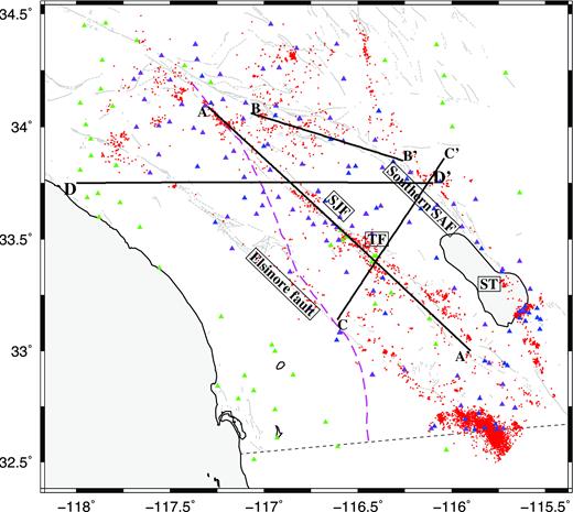
Map of the southern California plate boundary region. The blue, green and purple triangles show stations at which body wave, surface wave and both data sets are available, respectively. Red dots show earthquakes for body wave data used in this study. Major faults are shown as fine grey lines. The magenta dashed line shows the Peninsular Range compositional boundary. Black lines show the cross-sections in Figs 3 and 11. SAF, San Andreas Fault; TF, Trifurcation Area; SJF, San Jacinto Fault; ST, Salton Trough.
The obtained Vp/Vs from joint inversion with Vp/Vs parametrization shows several main geologically consistent features (Fig. 2). For example, the high Vp/Vs at shallow depths (<5 km) along the southern San Andreas fault (SSAF) indicates fault-related damage and sediments in the Salton Trough area, whereas the Vp/Vs along San Jacinto fault (SJF) and Elsinore fault is moderate except in the trifurcation area. The difference in Vp/Vs between the SSAF and the SJF reflects that the SSAF is a relatively old fault (Karato & Jung 1998) with broad fault-related damage, which could lead to larger amplification of seismic waves compared to most of the SJF (Ben-Zion & Aki 1990; Spudich & Olsen 2001).

Horizontal slices of the Vp/Vs model at different depths. The magenta dashed lines at 8, 10 and 12 km depth show the PRCB. Grey lines show the major fault traces.
A contrast in Vp/Vs with approximately linear geometry exists at 8–12 km depth across the southern part of the Peninsular Range compositional boundary (PRCB; Fig. 2). To the northeast of the PRCB there are areas of younger and more felsic continental crust associated with low Vp/Vs anomalies, whereas to the southwest there is mafic oceanic crust with relatively high Vp/Vs (Silver & Chappell 1988), which is only shown in the northern part of our model because of degraded resolution in the southern part along the PRCB. The northern SJF with the simplest geometry coincides partly with the PRCB (Fig. 2), suggesting that the fault may have exploited the compositional boundary (Magistrale & Sanders 1995; Langenheim et al.2004) that provides a mechanically weak interface (e.g. Weertman 1980; Ben-Zion 2001).
A significant anomaly with high Vp/Vs in the lower crust (>18 km depth) coincides with the SJF zone in the trifurcation area and then curves to the southwest (Fig. 2). This anomaly is spatially correlated with the deep boundary of the seismicity (Hauksson et al.2012; Fig. 3) in the SJF zone and is not obvious from Vp or Vs models (Fang et al.2016). The spatial extent of this Vp/Vs anomaly is also correlated with high heat flow in the southern SJF (Enescu et al.2009). The high Vp/Vs beneath the seismogenic zone may be associated with a ductile shear zone, which was hypothesized by Ross et al. (2017) to explain the complex structure and seismicity distribution in the trifurcation area. It may also indicate deep creep which leads to excess seismicity in this area (Wdowinski 2009). The anomalous Vp/Vs and high heat flow point to the existence of a weak zone that may contribute to the branching of the SJFZ in the trifurcation area into three major faults (Prescott & Nur 1981; Thatcher & England 1998). Moreover, most seismicity is located in the deeper part of the low Vp/Vs anomalies (Fig. 3), which may suggest high stress concentration in the deeper part of the seismogenic zone.
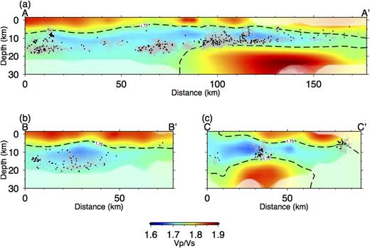
Vertical sections of Vp/Vs along different cross-sections shown in Fig. 1. (a) A–A′ along the SJF. (b) B–B′ along the southern SAF. (c) C–C′ perpendicular to the SJF across the trifurcation area. Grey and black dots represent the seismicity from Hauksson et al. (2012) and relocated earthquakes in this study, respectively.
4 DISCUSSION
4.1 Model assessment
Unlike Vp and Vs models from ray-theory-based tomography, for which an explicit relationship exists between observed data and model parameters, Vp/Vs models can only be obtained indirectly from P- and S-wave arrival times. Thus it is more difficult to assess the Vp/Vs models. Here we evaluate the performance of 3-D Vp/Vs models from different inversion strategies with synthetic tests and real data analysis.
Although checkerboard tests only approximately represent the model resolution and have theoretical drawbacks for uncertainty analysis (Lévěque et al.1993; Rawlinson et al.2014), we found it appropriate for comparison of different methods. We perform the checkerboard test by first constructing an input model with alternating high and low Vp/Vs anomalies with respect to the initial model. We then calculate traveltimes of body wave and frequency-dependent surface wave data using the same event and station distribution as the real data (Fig. 1) and add Gaussian random noise with a standard deviation of 2 per cent. This is followed by applying different inversion strategies mentioned in the methodology section to obtain the Vp/Vs models.
The obtained results show that the Vp/Vs model improved dramatically after incorporating surface wave dispersion data, both for direct division (Joint Vp–Vs) and for Vp/Vs parametrization (Joint Vp − κ). The latter also further reduces artefacts and stabilizes the Vp/Vs values, especially at greater depths (Fig. 4). In contrast, the recovery of the Vp/Vs model from the inversion with body wave data only is limited to the areas where data coverage is sufficient. There is an appearance of some recovery at all depths for the Vp/Vs model from directly dividing with body wave data only (Body Vp−Vs), but with a reversed sign of the anomalies , indicating incorrect amplitude estimation of either Vp or Vs. In order to eliminate effects resulting from different P- and S-wave coverage, we also selected P- and S-wave data from the same sources and stations to invert for Vp/Vs (Kennett et al.1998). The Vp/Vs model from restricted data with direct division (Subset body Vp−Vs) is comparable to that from Vp/Vs parametrization with only body waves, although it includes more artefacts. This synthetic test shows the Vp/Vs models differ greatly using different approaches. In contrast, the Vp and Vs models are generally consistent from the different inversion strategies (Figs 5 and 6).

Horizontal slices of the Vp/Vs model at 1, 8 and 17 km depths of input model (first column), joint inversion with Vp/Vs parametrization (second column), joint inversion with direct division (third column), body wave inversion with Vp/Vs parametrization (fourth column), body wave inversion with direct division (fifth column) and body wave inversion with comparable P- and S-wave data (sixth column). Grey lines show the major fault traces.

Horizontal slices of the checkerboard Vp model at 1, 8 and 17 km depths of the input checkerboard model (first column) and from joint inversion with Vp/Vs parametrization (second column), joint inversion with direct division (third column), body wave inversion with Vp/Vs parametrization (fourth column), body wave inversion with direct division (fifth column) and body wave inversion with comparable P- and S-wave data (sixth column).

Same as Fig. 5 but for Vs.
With the same process as for the checkerboard test, we also did a restoration test with the input model changed to the model inverted from the real data (Fig. 7). Here we only interpret the results qualitatively since this kind of synthetic test tends to be overly optimistic when it comes to accessing the uncertainty of the obtained model (Rawlinson et al.2014). The Vp/Vs model from body wave data only with Vp/Vs parametrization (Body Vp−κ) performs well. The joint inversion incorporating surface wave data improves the results, with more accurate amplitudes compared to the input model. Similar to the checkerboard test, the model from body wave data only with the direct division of Vp by Vs results in a reversed sign of Vp/Vs at shallow depths, both with full data sets (Body Vp−Vs) and selected data sets (Subset body Vp−Vs).

Same as Fig. 5 but for Vp/Vs from the restoration test.
The comparison of different approaches using real data also shows that joint inversion outperforms body wave inversion (Fig. 8), especially with Vp/Vs parametrization. Different from the synthetic tests, the Vp/Vs model at shallow depths from the direct division is misleading in the joint inversion, with a low Vp/Vs anomaly along the SSAF . The Vp/Vs contrast along the PRCB at shallow depths and high Vp/Vs anomaly in the lower crust in the Salton Trough region are not as evident as in the Vp/Vs model from Vp/Vs parametrization (Fig. 2). Surprisingly, both the Vp and Vs models seem reasonable, with low Vp and low Vs along the SSAF and similarity in terms of anomaly patterns (Figs 9 and 10). As the synthetic tests show, the body wave inversion with Vp/Vs parametrization performs well in the lower crust but resolution degrades at shallow depths, which is expected given the lack of constraint by short-period surface waves. The restricted data set, which consists of about 60 per cent of the original S wave and 35 per cent of the original P-wave data, stabilize the Vp/Vs model with less pronounced low Vp/Vs anomalies along the fault trace at shallow depths. Moreover, the model shows a similar high Vp/Vs anomaly at 17 km depth compared to the joint inversion with Vp/Vs parametrization, although it is still unreliable due to the poor data coverage.

Horizontal slices of the Vp/Vs model from the real data at 1, 8 and 17 km depths from joint inversion with direct division (first column), body wave inversion with Vp/Vs parametrization (second column), body wave inversion with direct division (third column) and body wave inversion with comparable P- and S-wave data (fourth column). The magenta dashed lines at 8 km depth show the PRCB. Grey lines show the major fault traces.

Horizontal slices of the Vp model at 1, 8 and 17 km depths from joint inversion with Vp/Vs parametrization (first column), joint inversion with direct division (second column), body wave inversion with Vp/Vs parametrization (third column), body wave inversion with direct division (fourth column) and body wave inversion with comparable P- and S-wave data (fifth column).

Same as Fig. 9 but for Vs.
4.2 The effect of surface wave sensitivity to Vp
Surface wave data are most sensitive to Vs, with small sensitivity to Vp and density. Thus the sensitivity of surface wave data to Vp and density is usually ignored, or incorporated into that of Vs according to an assumed empirical relationship in surface wave tomography (e.g. Yao et al.2008; Fang et al.2015). Since we have both body and surface wave data available, we can take full advantages of the sensitivity of surface waves to Vp and alleviate the trade-off between Vp, Vs and density by inverting for Vp and Vs simultaneously. Fig. 11 shows the comparison between two cases of considering or ignoring the Vp sensitivity of surface waves. It is clear that including Vp sensitivity results in better amplitude recovery, especially at shallow depths where the sensitivity of surface waves to Vp is large. This also leads to improvement at greater depths, although not substantially.

Cross-section of Vp/Vs of (a) input model, (b) synthetic data with Vp sensitivity and (c) without Vp sensitivity. The position is shown in Fig. 1.
4.3 The choice of different parametrizations
Although the Vp, Vs and Vp/Vs models can be obtained with different data sets and different parametrizations, they are not independent parameters. In other words, knowing either two can in principle determine the third one. Theoretically, different parametrizations would lead to the same results with ideal data coverage and known data noise. But in practice, it is generally not the case and the choice of different parametrizations usually depends on the parameters of interest. For example, direct Vp and Vs parametrization is preferred in cases where Vs is of main interest (Wagner et al.2006). In contrast, Vp/Vs parametrization could lead to a more stable Vp/Vs model, which can be directly related to partial melting, water content, lithology and so on. While it is better to test both parametrizations and then compare results, we suggest putting more emphasis on Vp/Vs parametrization if both parametrizations fit the data equally well, as in our case (Fig. 12). The synthetic test using Vp and Vs parametrization (Fig. 4) shows reversed signs of Vp/Vs but the Vp and Vs appear correct (Figs 5 and 6). In the real data case with the same parametrization, we observe low Vp/Vs along the southern SAF at shallow depth (Fig. 8), which is difficult to interpret, although both Vp and Vs show slow anomalies in the same region (Fang et al.2016). Thus we believe the Vs perturbations have been underestimated with the Vp and Vs parametrization, although the anomaly pattern seems reasonable.

Residual variation with iterations for (a) body wave data and (b) surface wave data in the joint inversion with Vp/Vs parametrization (blue lines) and direct division (red lines).
5 CONCLUSIONS
Analyses of different methods to obtain crustal Vp/Vs models indicate that jointly inverting both body and surface wave data could better constrain the Vp/Vs model, especially with Vp/Vs parametrizations. Synthetic tests confirm the results of Eberhart-Phillips (1990) and Michelini (1993) that Vp/Vs models from the direct division of Vp and Vs models tend to include artefacts, even when both Vp and Vs models are themselves reasonable. In contrast, joint inversion using both body and surface wave traveltime data can stabilize and improve the obtained Vp/Vs model, especially with the Vp/Vs parametrization approach. The derived Vp/Vs model in the southern California plate boundary region from joint inversion with Vp/Vs parametrization is consistent with the local geology, with high Vp/Vs at shallow depths along faults related to fault-related damage, a Vp/Vs contrast at mid-crustal depth correlating well with the PRCB and a high Vp/Vs in the lower crust in the Salton Trough region corresponding to the high heat flow in that region. Together with the absolute wave speed models, as well as other geophysical and geological constraints, the improved Vp/Vs model contributes to understanding regional tectonics, lithology and physical state in the crust of the southern California plate boundary region.
ACKNOWLEDGEMENTS
The manuscript benefited from constructive comments from two anonymous reviewers. The data used in this study are from Allam & Ben-Zion (2012) and Zigone et al. (2015) and they are available upon request. This research was supported by the Southern California Earthquake Center (Contribution No. 8909). SCEC is funded by NSF Cooperative Agreement EAR-1033462 and USGS Cooperative Agreement G12AC20038. HY acknowledges support from the National Natural Science Foundation of China (grant nos. 41790464 and 41574034). YBZ acknowledges support from the National Science Foundation (grant no.162061).
REFERENCES
,
