The rupture extent of low frequency earthquakes near Parkfield, CA

Hawthorne, Jessica C; Thomas, Amanda M; Ampuero, Jean-Paul

doi:10.1093/gji/ggy429

SUMMARY

The low frequency earthquakes (LFEs) that constitute tectonic tremor are often inferred to be slow: to have durations of 0.2–0.5 s, a factor of 10–100 longer than those of typical M_W 1–2 earthquakes. Here we examine LFEs near Parkfield, CA in order to assess several proposed explanations for LFEs’ long durations. We determine LFE rupture areas and location distributions using a new approach, similar to directivity analysis, where we examine how signals coming from various locations within LFEs’ finite rupture extents create differences in the apparent source time functions recorded at various stations. We use synthetic ruptures to determine how much the LFE signals recorded at each station would be modified by spatial variations of the source–station traveltime within the rupture area given various possible rupture diameters, and then compare those synthetics with the data. Our synthetics show that the methodology can identify interstation variations created by heterogeneous slip distributions or complex rupture edges, and thus lets us estimate LFE rupture extents for unilateral or bilateral ruptures. To obtain robust estimates of the sources’ similarity across stations, we stack signals from thousands of LFEs, using an empirical Green’s function approach to isolate the LFEs’ apparent source time functions from the path effects. Our analysis of LFEs in Parkfield implies that LFEs’ apparent source time functions are similar across stations at frequencies up to 8–16 Hz, depending on the family. The interstation coherence observed at these relatively high frequencies, or short wavelengths (down to 0.2–0.5 km), suggest that LFEs in each of the seven families examined occur on asperities. They are clustered in patches with sub-1-km diameters. The individual LFEs’ rupture diameters are estimated to be smaller than 1.1 km for all families, and smaller than 0.5 km and 1 km for the two shallowest families, which were previously found to have 0.2-s durations. Coupling the diameters with the durations suggests that it is possible to model these M_W 1–2 LFEs with earthquake-like rupture speeds: around 70 |$\hbox{ per cent}$| of the shear wave speed. However, that rupture speed matches the data only at the edge of our uncertainty estimates for the family with highest coherence. The data for that family are better matched if LFEs have rupture velocities smaller than 40 |$\hbox{ per cent}$| of the shear wave speed, or if LFEs have different rupture dynamics. They could have long rise times, contain composite sub-ruptures, or have slip distributions that persist from event to event.

Transient deformation, Earthquake source observations, Rheology and friction of fault zones, Continental tectonics: strike-slip and transform

1 INTRODUCTION

Tectonic tremor is a long-duration seismic signal, best observed at frequencies between 1 and 10 Hz (e.g. Obara 2002; Rogers & Dragert 2003; Payero et al.2008; Peterson & Christensen 2009; Rubinstein et al.2009; Fry et al.2011). It is thought to consist of numerous small low frequency earthquakes, or LFEs (Shelly et al.2006, 2007; Wech & Creager 2007; Brown et al.2009). LFEs are often inferred to have magnitudes between M_W 1 and 2.5 but to have corner frequencies of a few Hz, a factor of 10–100 times smaller than corner frequencies observed for ‘normal’ M_W 1–2.5 earthquakes (Fletcher & McGarr 2011; Zhang et al.2011; Bostock et al.2017). LFEs are found to have durations around 0.2 s in Parkfield (Thomas et al.2016) and around 0.5 s in Cascadia (Bostock et al.2015), which are a factor of 10–100 longer than ‘normal’ M_W 1–2.5 earthquakes.

1.1 Potential causes of LFEs’ Long durations

The durations of normal earthquakes are determined by their spatial extent: by how long it takes the rupture to progress across the earthquake area. Models and observations suggest that earthquake ruptures usually progress at speeds of 2–3 km s^–1, or 60–95 |$\hbox{ per cent}$| of the shear wave speed V_s (Kanamori & Brodsky 2004; McGuire 2004; Madariaga 2007; Seekins & Boatwright 2010; Taira et al.2015; Folesky et al.2016; Ye et al.2016; Melgar & Hayes 2017; Chounet et al.2018). Earthquakes’ durations can thus be roughly estimated by dividing their rupture lengths by the shear wave speed. If LFEs, like normal earthquakes, rupture at speeds close to the shear wave speed, their long durations could indicate that LFEs have unusually large lengths given their moment: perhaps 0.7–1.5 km. In this scenario, LFEs would have lower stress drops than normal earthquakes: 0.1–10 kPa, but they could otherwise be governed by the same physical processes. LFEs could be driven by unstable frictional sliding, and their slip speeds could be limited by the energy that they dissipate via seismic waves (e.g. Rice 1980; Kanamori & Brodsky 2004).

However, it is also possible that seismic wave generation has minimal impact on LFE dynamics and that LFEs are governed by different fault zone processes. LFEs’ slip rates may be limited by a spatial constraint or by a speed-limiting frictional rheology (e.g. Liu & Rice 2005, 2007; Shibazaki & Shimamoto 2007; Rubin 2008; Segall et al.2010; Skarbek et al.2012; Fagereng et al.2014; Yabe & Ide 2017). For instance, LFEs could occur on faults with a velocity-strengthening rheology, which inhibits increases in slip rate. The brief slip rate increases seen in LFEs could result from imposed local stress concentrations, perhaps created by the creep fronts of large slow slip events (e.g. Perfettini & Ampuero 2008; Rubin 2009). Alternatively, LFEs could occur on faults with a more complex rheology, which encourages initial increases in slip rate but inhibits slip rates higher than some cutoff speed. Such rheologies are commonly proposed for slow slip events and may be created by shear-induced dilatancy or by a minimum asperity size (e.g. Shibazaki & Iio 2003; Shibazaki & Shimamoto 2007; Liu et al.2010; Segall et al.2010; Hawthorne & Rubin 2013; Poulet et al.2014). The possibility that LFEs are small versions of slow slip events is intriguing because slip rates vary widely from slow slip to tremor (Ide et al.2007, 2008; Aguiar et al.2009; Gao et al.2012; Ide & Yabe 2014; Hawthorne & Bartlow 2018). Several of the processes proposed to govern slow slip would have difficulty producing such a wide range of slip rates (e.g. Liu & Rice 2005, 2007; Shibazaki & Shimamoto 2007; Hawthorne & Rubin 2013; Fagereng et al.2014; Veveakis et al.2014). If LFE slip rates are limited primarily by frictional resistance to shear and not by seismic wave radiation, LFEs need not rupture across the fault at speeds close to the shear wave speed. They could rupture more slowly and have diameters far smaller than 1 km despite their 0.2-s durations.

LFEs could also have small rupture diameters if their 0.2-s durations and low corner frequencies are actually apparent values, not true values. LFEs could be ‘normal’ M_W 1–2.5 earthquakes, with 0.01-s durations and 10-m rupture diameters. They may appear to be dominated by low-frequency signals only because their high-frequency signals are attenuated when they pass through a highly damaged fault zone or through a region of high pore fluid pressure (Gomberg et al.2012; Bostock et al.2017). Regions of high pore pressure or increased attenuation are frequently identified near the slow slip region (Audet et al.2009; Song et al.2009; van Avendonk et al.2010; Kato et al.2010; Fagereng & Diener 2011; Kitajima & Saffer 2012; Nowack & Bostock 2013; Yabe et al.2014; Saffer & Wallace 2015; Audet & Schaeffer 2018), though we note that any regions with attenuation strong enough to produce tremor’s frequency content might have to be localized into patches. Earthquakes do occur below the tremor-generating region, and some of them show higher-frequency signals than tremor (Seno & Yamasaki 2003; Shelly et al.2006; Bell et al.2010; Kato et al.2010; Ohta & Ide 2011; Gomberg et al.2012; Bostock et al.2017).

1.2 Potential role of tremor asperities

Tremor is often patchily distributed along the plate interface; it is densely concentrated in some regions but appears absent in others (e.g. Payero et al.2008; Maeda & Obara 2009; Walter et al.2011; Ghosh et al.2012; Armbruster et al.2014). Some observations and models suggest that tremor occurs only on a set of tremor-generating asperities (e.g. Ariyoshi et al.2009; Ando et al.2010, 2012; Shelly 2010b; Nakata et al.2011; Sweet et al.2014; Veedu & Barbot 2016; Chestler & Creager 2017a,b; Luo & Ampuero 2017). Such asperities may also be suggested by the success of template matching approaches to tremor identification, in which LFEs are detected and grouped into families according to waveform similarity. Each LFE family could reflect an individual tremor asperity (Shelly et al.2007; Brown et al.2008; Bostock et al.2012; Frank et al.2013; Kato 2017; Shelly 2017). However, the family grouping could also result from more gradual variations in the path effects. LFEs located more than 1 or a few km away from each other may be grouped into distinct families simply because the path effects vary significantly on several-km length scales, so that well-separated LFEs give rise to distinct seismograms.

A few studies have provided further indications that at least some LFE families are created by clusters of tremor. Sweet et al. (2014) relocated LFEs within an isolated family in Cascadia and found that they clustered within a 1-km-wide patch. Chestler & Creager (2017b) relocated LFEs within around 20 families in Cascadia and found that LFEs cluster within 1–2-km-wide patches that are often separated by >5-km-wide areas with few to no LFEs, or at least few to no detected LFEs. Tremor-generating asperities are also suggested by the highly repetitive recurrence intervals of one isolated LFE family near Parkfield, CA. The consistent rupture intervals suggest that the LFEs could be repeating similar ruptures of a particular asperity (Shelly 2010b; Veedu & Barbot 2016). Repetitive LFE rupture is also suggested by LFE moments and durations that vary little from event to event, creating exponential amplitude distributions (Watanabe et al.2007; Shelly & Hardebeck 2010; Chamberlain et al.2014; Sweet et al.2014; Bostock et al.2015; Chestler & Creager 2017a), though it is also possible that each LFE ruptures only a portion of a tremor-generating asperity. The total slip on an LFE patch could result from a range of ruptures of different types, as well as some aseismic slip (Chestler & Creager 2017a).

1.3 Analysis to be presented

In this study, we further assess whether small asperities control tremor generation and whether LFEs are governed by earthquake-like or slow slip rheologies. We determine the rupture extents of LFEs in seven families near Parkfield, CA and place upper bounds on the spatial distribution of LFEs in each family and on the average LFE rupture area. In order to obtain these bounds, we will introduce a new coherence-based approach, which can be thought of as a version of directivity analysis that we have modified so that we can combine data from thousands of LFEs which may rupture unilaterally or bilaterally (e.g. Mueller 1985; Mori & Frankel 1990; Got & Fréchet 1993; Velasco et al.1994; Lengliné & Got 2011; Wang & Rubin 2011; Kane et al.2013). We examine how signals coming from various locations within LFEs’ finite rupture areas can produce complex apparent source time functions (ASTFs) that vary from station to station. We quantify the ASTF variation as a function of frequency, or seismic wavelength, in order to determine the LFE rupture area.

We qualitatively explain how the ASTFs’ frequency-dependent variability should reflect LFEs’ rupture extents in Section 2. In Section 3, we present our approach in more detail. We describe how we can isolate the ASTFs from observed seismograms using an empirical Green’s function approach and then describe how we can quantify the ASTFs’ coherence among LFEs and among stations. In Sections 4 and 5, we analyse ASTF coherence for individual LFEs near Parkfield and then average over thousands of LFEs to obtain well-resolved estimates of interstation coherence as a function of frequency. For comparison, we also compute ASTF coherence for a suite of synthetic LFEs with a range of diameters and rupture velocities (Section 6). Finally, in Sections 7 and 8, we compare the data with the synthetics to determine which rupture areas are plausible and which types of LFEs could match the observations.

2 PREMISE: MAPPING INTERSTATION SIMILARITY TO RUPTURE AREA

In order to estimate LFE areas, we note that seismic waves generated at a range of locations throughout the source region require different amounts of time to travel to the various stations. For instance, in the rupture illustrated in Fig. 1(d), seismic waves generated by the high-slip asperity marked in red arrive earliest at the NW station (left) because the asperity is located in the northwestern half of the rupture. But waves generated at the blue asperity, located farther SE (right), arrive first at the SE station. The time-shifted signals give rise to apparent source time functions (ASTFs) that differ among the recording stations, as seen in Figs 1(a)–(c).

Figure 1.

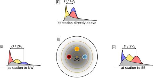
(a–c) ASTFs observed at three stations due to rupture of the slip distribution illustrated with grey and coloured shading in panel (d). Rupture progresses outward from the center and moves through three high-slip asperities of varying magnitude, illustrated with coloured circles. The asperities generate seismic waves which require different amounts of time to travel to the stations, giving rise to the various coloured peaks in the ASTFs. Note that the timing of the asperity-created peaks varies among the stations by up to D/2V_s: by half the rupture diameter divided by the shear wave speed.

Open in new tab Download slide

If we assume that Earth structure is relatively uniform within the source region, we may account for the traveltime variations by modeling the observed seismograms d_k in terms of station-specific apparent source time functions s_k. At each station k,

\begin{eqnarray*} \skew8\hat{d}_{k}(\omega )=\hat{s}_{k}(\omega )\hat{g}_k(\omega ). \end{eqnarray*}

(1)

Here g_k is an average Green’s function for the source area, and |$\skew8\hat{d}_{k}$|⁠, |$\hat{s}_{k}$|⁠, and |$\hat{g}_k$| are the Fourier coefficients of d_k, s_k, and g_k, respectively.

The ASTFs s_k can be computed by integrating time-shifted versions of the slip rate functions over the rupture area. If g_k(t) is taken as the Green’s function for a reference location x₀, and if |$\dot{\delta }(x,t)$| is the slip rate as a function of location x and time t, and Δt_k(x) is the source–station traveltime for a signal generated at location x,

\begin{eqnarray*} s_k(t) = \int _{\textrm{rupture~area}} \dot{\delta }(x,t-\Delta t_k(x)+\Delta t_k(x_0)) dA. \end{eqnarray*}

(2)

The colouring in Fig. 1 shows how the three slip asperities shown contribute to ASTFs that differ among stations located to the northwest, southeast, and above the earthquake. Note that the asperities create differences at all three stations even though the earthquake ruptures radially out from the centre point.

There is, however, a limit to the ASTF differences. The spatially variable source–station traveltime may shift peaks in this earthquake’s source time function by only a limited amount: up to D/V_s, the rupture diameter D divided by the seismic wavespeed V_s. Thus we can see differences in the ASTFs only if we examine their short-period signal. If we examine ASTFs at periods much longer than D/V_s, the traveltime shifts will be a small fraction of the period, and the ASTFs will be roughly the same at all stations. Synthetic rupture models described in Section 6 show that ASTFs are similar among stations at periods longer than 0.45 to 1.4D/V_s. Here the range of limiting periods results from the earthquakes’ other rupture parameters, but we note that the limiting periods depend primarily on the diameter divided by seismic wave speed V_s, not on the diameter divided by the LFEs’ rupture speed V_r. We will thus be able to use the ASTFs’ frequency-dependent similarity to estimate LFE rupture extents without making restrictive assumptions about LFE rupture dynamics.

3 QUANTIFYING COHERENCE ACROSS EVENTS AND STATIONS

3.1 Removing the path effect

In order to examine ASTFs, we must first isolate them from the observed seismograms. To do so, we use an empirical Green’s function approach similar to that of Hawthorne & Ampuero (2017) and compare each LFE’s seismograms with a template event created via stacking (a variant on, e.g. Mueller 1985; Mori & Frankel 1990; Velasco et al.1994; Hough 1997; Prieto et al.2004; Baltay et al.2010; Kwiatek et al.2011; Uchide et al.2014). Both the seismograms d_jk of the individual LFEs j and the seismograms d_tk of the templates t can be approximated as convolutions of ASTFs s_jk or s_tk and Green’s functions g_k, so that, in the frequency domain,

\begin{eqnarray*} \skew8\hat{d}_{jk}(\omega )=\hat{s}_{jk}(\omega )\hat{g}_k(\omega ). \end{eqnarray*}

(3)

To isolate the ASTFs from the Green’s functions, we compute the normalized cross-spectrum |$\hat{x}_{jk}$| of the individual and template records:

\begin{eqnarray*} \hat{x}_{jk} = \frac{\skew8\hat{d}_{jk} \skew8\hat{d}^*_{tk}}{|\skew8\hat{d}^*_{tk}|^2} = \frac{\hat{s}_{jk} \hat{s}^*_{tk} |\hat{g}_{k}|^2}{|\hat{s}_{tk}|^2 |\hat{g}_{k}|^2} = \frac{\hat{s}_{jk} \hat{s}^*_{tk}}{|\hat{s}_{tk}|^2}, \end{eqnarray*}

(4)

where * denotes the complex conjugate, and we have omitted the frequency indexing for readability. In the second equality, we have assumed that the template LFE has the same Green’s functions as the individual event. In this case, the path effects cancel out, and we are left with a function that depends on the relative amplitudes and phases of the individual and template ASTFs. Note that we always normalize by the template amplitude, as this will allow us to stack ASTFs from thousands of LFEs, and to use the cross-spectra |$\hat{x}_{jk}$| to examine how ASTFs’ amplitudes and phases vary among LFEs j and stations k.

3.2 ASTF energy: direct and interstation coherence

As a first step in our analysis, we ignore interstation variations, and simply examine how much LFE source time functions vary from event to event. We assess the similarity between the individual and template ASTFs by computing the directly coherent power for each LFE j:

\begin{eqnarray*} P_d &=& \frac{1}{N} \sum _{k=1}^N{a^2_{jk} \left[\operatorname{Re}\left(\hat{x}_{jk}\right)\right]^2 \operatorname{sgn} \left[\operatorname{Re}\left(\hat{x}_{jk}\right)\right] } \\ &=& \frac{1}{N} \sum _{k=1}^N{a^2_{jk} \left[\operatorname{Re}{\frac{\hat{s}_{jk} \hat{s}^*_{tk}}{|\hat{s}_{tk}|^2}}\right]^2 \operatorname{sgn} \left[\operatorname{Re}{\left(\hat{s}_{jk} \hat{s}^*_{tk}\right)}\right]}. \end{eqnarray*}

(5),(6)

Here the coefficients a_jk represent a weighting of the LFE records, which we will use to downweight noisy seismograms (Section 4.3).

The equality in eq. (6) assumes that the individual LFE and the template have the same path effects. If the individual and template LFEs have the same path effects, and in addition have similar and well-aligned ASTFs |$\hat{s}_{jk}$| and |$\hat{s}_{tk}$|⁠, so that the value |$\hat{s}_{jk} \hat{s}^*_{tk}$| in eq. (6) is real and positive, then the directly coherent power P_d will be positive. Its amplitude will be determined by the relative power of the individual and template ASTFs.

The relative ASTF power also determines the amplitude of the interstation coherent power P_c. With this power calculation, we seek to ignore ASTF variations across events, and instead assess the ASTFs’ similarity across stations. So we compute (see Section S1 for computational details)

\begin{eqnarray*} P_c &=& \frac{2}{N(N-1)} \sum _{k=1}^N \sum _{l=k+1}^N{a_{jk}a_{jl} \operatorname{Re}\left(\hat{x}_{jk} \hat{x}_{jl}^*\right)} \\ &=& \frac{2}{N(N-1)} \sum _{k=1}^N\sum _{l=k+1}^N{a_{jk}a_{jl} \operatorname{Re}{\frac{\left(\hat{s}_{jk}\hat{s}^*_{jl}\right) \left(\hat{s}^*_{tk}\hat{s}_{tl}\right)}{|\hat{s}_{tk}|^2|\hat{s}_{tl}|^2}}}, \end{eqnarray*}

(7),(8)

where the second equality again assumes common path effects and where the summation is across pairs of the N stations, indexed k and l. As noted in Section 2, the ASTFs are expected to be the same for all stations if the period being considered with these Fourier coefficients is long compared with D/V_s, the intrasource seismic wave traveltime. If the ASTFs are the same across stations at the period of interest, we will have |$\hat{s}_{jk} = \hat{s}_{jl}$| and |$\hat{s}_{tk} = \hat{s}_{tl}$|⁠, so that all three of |$\hat{s}_{jk}\hat{s}^*_{jl}$|⁠, |$\hat{s}^*_{tk}\hat{s}_{tl}$|⁠, and P_c are real and positive.

P_d and P_c thus give us estimates of the direct or interstation coherent power of an LFE, as normalized by the template power. However, we can obtain a more interpretable normalization if we also estimate the full template-normalized LFE power, including any incoherent contributions:

\begin{eqnarray*} P_l &=& \frac{1}{N} \sum _{k=1}^N a_{jk}^2 |\hat{x}_{jk}|^2 \\ &=& \frac{1}{N} \sum _{k=1}^N{a_{jk}^2\frac{|\hat{s}_{jk}|^2}{|\hat{s}_{tk}|^2}}. \end{eqnarray*}

(9),(10)

We will use the LFE power P_l to normalize P_d and P_c and compute the fraction of the power that is coherent across events and stations.

4 CALCULATING POWERS OF PARKFIELD LFES

When we extract the coherent and incoherent powers of LFEs near Parkfield, we will also have to estimate and remove the power contributed by noise, and we will have to average over thousands of LFEs to obtain well-resolved powers. To begin, we describe the LFE catalog and seismic data (Section 4.1) and create templates for seven LFE families (Section 4.2). Then we demonstrate our approach by estimating template-normalized powers for an individual LFE (Section 4.3). Finally, we average the powers over the LFEs in each family (Section 5).

4.1 Data and LFE families

The LFEs considered here occurred between 2006 and 2015 at depths of 16–23 km near Parkfield, CA (see Fig. 2). They were identified via cross-correlation by Shelly (2017) as part of his 15-yr tremor catalogue and are grouped into seven families numbered 37140, 37102, 70316, 27270, 45688, 77401, and 9707, with 2500–8300 LFEs in each family (see also Shelly et al.2009; Shelly & Hardebeck 2010). LFEs in families 37140 and 37102 were examined by Thomas et al. (2016) and found to have best-fitting source durations of 0.19 and 0.22 s, respectively. We use LFE seismograms from 17 borehole seismic stations in the Berkeley HRSN (High Resolution Seismic Network) and in the PBO (Plate Boundary Observatory) network. Since this analysis relies on high-quality records of small LFEs, we correct the data for some errors identified by Shelly (2017). We have also gone through the data from each station and channel and discarded weeks- to years-long intervals where the LFE amplitudes vary more strongly than usual from event to event, as these intervals likely have larger-than-average noise.

Figure 2.

(a) Map view and (b) depth section of the LFE families (blue stars), local M > 2.5 earthquakes (circles), and the HRSN and PBO seismic stations used (triangles). Earthquake sizes are scaled to the radii expected for 3-MPa stress drops, and locations are taken from the NCSN catalogue and the relocations of Waldhauser (2009).

Open in new tab Download slide

4.2 Stacked LFE templates

For each LFE family, we create a low-noise template by averaging the LFE records for each channel. We bandpass filter the LFE seismograms from 2 to 30 Hz, normalize them by their maximum values, and then average, weighting each record by the station-averaged cross-correlation coefficient obtained by Shelly (2017). Then we rescale these normalized stacks so that their amplitudes match the amplitudes of individual records, as described in Section S2.

We iterate the stack four times to be sure that the stacks’ amplitudes are stable and to improve the signal to noise ratio by of order 10|$\hbox{ per cent}$|⁠. In each interation, we discard records with very small or unusual amplitudes (for details see Section S2).

We estimate the signal to noise ratio of the stacks using a 3-s window starting just before the S arrival. We keep only the stacks which have average amplitude spectra at least three times larger than the noise in the 2–10 Hz band. The procedure leaves us with 16–29 well-resolved template seismograms for each LFE family, observed on the two horizontal components of 9–16 stations. Some templates are shown in Fig. 3(a), and the whole set of templates is shown Figs S1–S7.

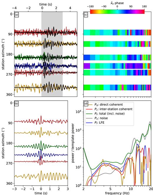
$(a) Some of the template seismograms (black) for family 37102 along with seismograms observed for one LFE (colour). Traces are organized according to the station’s azimuth relative to the LFE and are scaled to their maximum value. The grey shading indicates the portion of the template that is correlated with the individual observations. (b) Cross-correlations of the observed seismograms with the template. (c) Phase of the cross-spectra $\hat{x}_k$: of the Fourier coefficients of the cross-correlations in panel b. (d) Yellow, red and green curves: Pd, Pc and Pt—the coherent and total template-normalized powers from the LFE interval. Grey: Pn—the noise power, computed in an interval without the LFE. Blue: Pl = Pt − Pn—the power likely contributed by the LFE. Note that with just this one LFE, it is not practical to interpret the relative values of the coherent and total powers.$

Figure 3.

(a) Some of the template seismograms (black) for family 37102 along with seismograms observed for one LFE (colour). Traces are organized according to the station’s azimuth relative to the LFE and are scaled to their maximum value. The grey shading indicates the portion of the template that is correlated with the individual observations. (b) Cross-correlations of the observed seismograms with the template. (c) Phase of the cross-spectra |$\hat{x}_k$|⁠: of the Fourier coefficients of the cross-correlations in panel b. (d) Yellow, red and green curves: P_d, P_c and P_t—the coherent and total template-normalized powers from the LFE interval. Grey: P_n—the noise power, computed in an interval without the LFE. Blue: P_l = P_t − P_n—the power likely contributed by the LFE. Note that with just this one LFE, it is not practical to interpret the relative values of the coherent and total powers.

Open in new tab Download slide

4.3 Coherent and total powers for one LFE

We will use the obtained templates to remove the Green’s functions from individual LFE records, so that we can probe the LFEs’ ASTFs. To prepare, we realign each LFE’s origin time to better match the template, as poor alignment can reduce the direct coherence P_d. We bandpass filter to 2–5 Hz, cross-correlate to obtain a preferred shift at each station, and then shift the seismograms of all stations by the median shift.

Next, we remove the path effects to facilitate the power calculations. We extract 3-s-long segments of the template seismograms, starting just before the S arrival, and cross-correlate the segments with the individual LFE records. The individual LFE records are truncated 0.2 s before the S arrival to reduce contamination by the P arrival, but they are not truncated after theS wave. We average the cross-correlations over the available channels at each station.

Cross-correlations obtained for one LFE are illustrated in Fig. 3(b). The cross-correlations are often roughly but not entirely symmetric, suggesting that the individual and template LFEs have slightly different source time functions. The asymmetry is also apparent in the non-zero phases of the cross-correlations’ Fourier coefficients, which are equal to the phases of the normalized cross-spectra |$\hat{x}_{jk}$| (eq. 4, Fig. 3c). To estimate the |$\hat{x}_{jk}$|⁠, we first extract a 6-s portion of the cross-correlations, multiply by a Slepian taper concentrated at frequencies lower than 0.4 Hz, and compute the Fourier transform (Thomson 1982). Then we normalize; we divide by the Fourier transform of the template seismograms’ autocorrelation, computed via the same procedure.

We use the cross-spectra |$\hat{x}_{jk}$| to compute the power that is directly coherent (P_d, eq. 5) and coherent among stations (P_c, eq. 7) and plot them in yellow and red in Fig. 3(d). The total power P_t in the template-normalized cross-correlation is also computed, following eq. (9), and is plotted in green. However, a significant fraction of this total power comes from noise, not from the LFE signal. To estimate the noise contribution, we cross-correlate the template seismograms with data from noise intervals starting 8 s before the S arrivals. We compute the power (P_n) in those noise correlations, again following eq. (9), and plot it in grey in Fig. 3(d). Finally, we subtract the noise power P_n from the total power P_t to determine the power contributed by the LFE (P_l, blue in Fig. 3d).

In all the power calculations, we use weightings a_jk equal to one divided by the standard deviation of the 2–30-Hz filtered waveform, as computed in the 4 s ending 0.5 s before the LFE S arrival. This weighting reduces the importance of seismograms with large noise and allows us to better identify the LFEs’ coherence. Note that uniform weightings (a_jk = 1) would result in lower coherence because a larger fraction of calculated powers would be contributed by noise, which is incoherent among stations. We choose weightings a_jk that depend on the signal between 4.5 and 0.5 s before the S arrival because these a_jk provide reasonable estimates of the noise, but they do not bias any of the power calculations, as all of the power in P_t, P_c and P_d comes from after 0.2 s before the S arrival and almost all of the subtracted noise power P_n comes from more than 5 s before the S arrival. Note that the P-wave signal is small enough to be neglible. It never contributes more than a few percent of the power in the 4 s before the S arrival.

In an ideal scenario, we would now interpret the powers estimated for this LFE, and compare the coherent powers P_d and P_c with the LFE power P_l. However, for this and other individual LFEs, the powers are too poorly resolved to allow direct interpretation. In Fig. 3(d), the ratios P_d/P_l and P_c/P_l vary by tens of per cent among the frequencies but show no systematic trend, and there is further variation if we use different subsets of the stations. So in the next section, we will average the powers over several thousand LFEs to obtain well-resolved and stable coherent power fractions.

5 RESULTS: EVENT-AVERAGED COHERENT AND INCOHERENT POWERS

To estimate P_c, P_d, P_t and P_n for a given family of LFEs, we compute the powers for each event in the family and then average. However, some LFE records have exceptionally large noise, so we check the signals’ amplitudes before the calculation and discard records when the S arrival or the preceding noise interval has standard deviation that differs by more than a factor of 10 from that channel’s median. This record selection, coupled with data availability, leaves us with 860–4220 LFEs per family which have template-normalized powers computed from at least five stations.

Fig. 4(a) shows the summed coherent and total powers obtained from 2000 LFEs in family 37140, one of the two families with duration estimates from Thomas et al. (2016). The shading indicates 95 |$\hbox{ per cent}$| uncertainty ranges on the powers, obtained by bootstrapping the LFEs included in the summation. All of the template-normalized powers increase with frequency, suggesting that the high-frequency template power is damped relative to a typical LFE. The stacks’ high-frequency signal may be averaged out by stacking if LFEs are more different at higher frequencies or if the LFE timing is not accurate enough to allow coherent stacks at higher frequencies. The stacking effectively creates a template LFE which has slightly broader and simpler ASTFs (Royer & Bostock 2014). This ASTF modification will reduce the direct coherence between the template and the individual LFEs P_d/P_l. However, smoothing the template ASTF in the same way at all stations should not affect P_c, as P_c is independent of interevent ASTF differences. The ASTF averaging should reduce the interstation coherence P_c/P_l only if the stacks’ constituent LFEs are distributed in space, so that the station-dependent source–station arrival times vary among the LFEs. Stacking the shifted signals of such distributed LFEs would smooth the templates’ ASTFs differerently at different stations and could lead to reduced P_c/P_l.

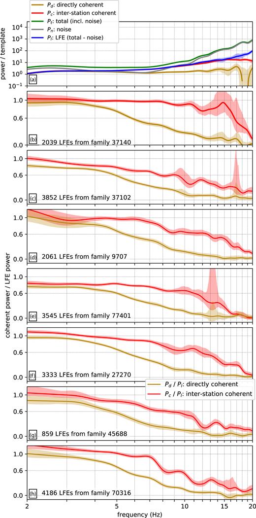
$(a) Coherent and incoherent powers, as in Fig. 3(d), but averaged over 2000 LFEs from family 37140. Colour indicates the power of interest. In all panels, the line indicates the value obtained with all allowable LFEs, and the shaded region delimits 95 $\hbox{ per cent}$ confidence intervals obtained by bootstrapping the included events. (b–h) Ratios of the direct and interstation coherence: Pc/Pl (yellow) and Pd/Pl (red). Each panel is computed for a different LFE family, as indicated by the text in the bottom left.$

Figure 4.

(a) Coherent and incoherent powers, as in Fig. 3(d), but averaged over 2000 LFEs from family 37140. Colour indicates the power of interest. In all panels, the line indicates the value obtained with all allowable LFEs, and the shaded region delimits 95 |$\hbox{ per cent}$| confidence intervals obtained by bootstrapping the included events. (b–h) Ratios of the direct and interstation coherence: P_c/P_l (yellow) and P_d/P_l (red). Each panel is computed for a different LFE family, as indicated by the text in the bottom left.

Open in new tab Download slide

We compute the coherent power fractions P_d/P_l and P_c/P_l for all seven families and plot the results in Figs 4(b)–(h). For family 37140 (panel b), the direct coherence P_d/P_l is larger than 0.8 at frequencies of 2–4 Hz, suggesting that most 0.2-s-long LFE source time functions are similar when viewed at these frequencies. We should note, however, that P_d/P_l may be slightly higher than its true value in this range because we allowed for an LFE origin time-shift using data in the 2–5 Hz range. P_d/P_l decreases at higher frequencies, falling below 0.6 at a frequency of 5 Hz. The decrease in direct coherence could imply (1) that the LFE source time functions are more different at higher frequencies, (2) that the LFEs are too poorly aligned to show direct coherence at high frequencies, or (3) that the stacking has modified the source time functions being compared. We have tried improving the alignment by using higher-frequency signals in the alignment cross-correlation, outside the 2–5 Hz range. We find that using higher frequencies in the alignment does result in large P_d/P_l out to higher frequencies, but we choose not to use that alignment here because some of the increase in P_d/P_l could come from the alignment of high-frequency noise.

Family 37140’s interstation coherent power P_c/P_l is insensitive to the alignment, and it remains coherent over a wider frequency range. P_c/P_l is above or around 0.8 at frequencies up to 15 Hz and falls below 0.6 only at 16.5 Hz. The persistence of high P_c/P_l out to frequencies >15 Hz suggests that the ASTFs vary little among stations at >0.07-s periods. We will use synthetic rupture calculations to interpret this high-frequency coherence in terms of LFE rupture area in Section 7.

The other six LFE families show slightly lower coherence, as seen in Figs 4(c)–(h) and in Figs S(8)–S14. Family 37102, the other family with an estimated duration (Thomas et al.2016), displays gradually decaying P_d/P_l and P_c/P_l (Figs 4 b and S9). Its P_d/P_l falls below 0.6 at 4 Hz, and its P_c/P_l stays above or hovers near 0.6 until 9 Hz. For the remaining families, the direct coherence P_d/P_l remains above 0.6 out to 4–5 Hz. The interstation coherence P_c/P_l remains above 0.6 out to 8–13 Hz: to 8, 9, 11, 12 and 13 Hz.

These high-coherence frequency limits are likely lower bounds on the true high-coherence frequencies. Our coherence estimates could be affected by a range of factors, including LFE clustering, data selection, LFE origin time alignment, and template accuracy. We describe the uncertainties in Appendix and note that only the LFE origin time alignment is likely to give artificially high coherence, and it affects only P_d/P_l, not P_c/P_l. The remaining factors would result in our underestimating the true P_d/P_l and P_c/P_l. In Section 7, we will therefore interpret our coherence estimates as lower bounds on the true coherence when we consider the estimates’ implications for LFE rupture areas and location distributions.

6 FREQUENCIES WITH COHERENT POWER: SYNTHETICS

To consider the coherence’s implications for LFE rupture areas, we need to know how P_d/P_l and P_c/P_l depend on LFE rupture properties. So we generate and analyse groups of synthetic LFEs with various diameters D, rupture velocities V_r, and rise times t_r. We create synthetic ruptures for three types of LFEs (Section 6.1), analyse their waveforms (Section 6.2), and examine the coherent frequencies as a function of the LFE properties (Section 6.3).

6.1 Synthetic LFEs models

We create and analyse groups of 100 LFEs. The individual events are assigned diameters D, rupture velocities V_r, and rise times t_r that cluster around specified mean values. The diameters, rupture velocities and rise times are chosen from lognormal distributions with factor of 1.3, 1.1 and 1.3 standard deviations, respectively. Moments are chosen from lognormal distributions with factor of 1.5 standard deviation and assigned with no consideration of the radii.

In the simplest version of our LFEs, each event is assigned a random heterogeneous slip distribution within a roughly circular area, as detailed in Section S4 and motivated by inferences of fractal earthquake slip distributions (Frankel 1991; Herrero & Bernard 1994; Mai & Beroza 2002). Rupture initiates at a random location within 0.4D of the centre and spreads radially at rate V_r. Once a location starts slipping, slip accumulates following a regularized Yoffe function with duration t_r (Tinti et al.2005).

We also construct groups of LFEs with more repetitive rupture patterns, as it is possible that LFEs within a given family recur not just on the same patch, but with similar rupture patterns within that patch (e.g. Ariyoshi et al.2009; Ando et al.2010; Sweet et al.2014; Chestler & Creager 2017b). In our repetitive LFEs, slip is the sum of two heterogeneous distributions: one that varies randomly from event to event and one that is the same from event to event. The distributions are scaled so that the repetitive component contributes twice as much moment, and slip always nucleates within 0.1D of the LFE centre points.

Finally, we construct groups of composite LFEs, as it is possible that individual LFEs comprise a series of small ruptures of the complex fault zone at depth (Fagereng et al.2014; Hayman & Lavier 2014; Chestler & Creager 2017b; Rubin & Bostock 2017). Each of our relatively crude composite LFEs contains five simple ruptures whose rupture velocities, diameters, and slip distributed are chosen from the lognormal and heterogeneous distributions described above. The five sub-ruptures begin at random times within a 2.5D/V_r interval.

6.2 Computing and analysing LFE waveforms

Having defined the location and timing of slip in the LFEs, we compute ASTFs for nearby stations. We assume that the synthetic LFEs are in the location of family 37140 and calculate ASTFs for the 12 stations used in its analysis, as shown in Figs 2 and S1. To calculate ASTFs, we integrate the slip rate over the slipping area at each time step, but shift the signals’ arrival times to account for the traveltime from each point in the source region to the observing stations, as in eq. (2). To calculate seismograms, we convolve these ASTFs with fake Green’s functions, which are taken to be white noise tapered by an exponential with a 3-s decay constant. We obtain similar results, with maximum coherent frequencies 10–20 |$\hbox{ per cent}$| smaller, if we take instead take local earthquake records as the Green’s functions to create synthetic seismograms (Fig. S26).

We may now process the synthetic seismograms. As with the real data, we create templates for each LFE group, normalizing the synthetic seismograms by their maximum values and stacking. We iterate the stacks three times. Each time, we cross-correlate the template seismograms with the individual LFEs’ waveforms. We identify a station-averaged time shift for each LFE, realign according to those shifts and stack.

Next, we use the templates to compute the cross-spectrum |$\hat{x}_{jk}$| for each synthetic LFE record (eq. 4). As with the real data, we compute the cross-spectra from the tapered cross-correlations, but we adjust the taper duration to ensure that it is always significantly longer than the LFEs’ durations. Finally, we compute the LFEs’ template-normalized powers P_c, P_d and P_l (eqs 5, 7 and 9). Figs 5(a), (c) and (e) shows the coherent power fractions P_d/P_l and P_c/P_l obtained for simple LFEs with various diameters, rupture velocities and rise times.

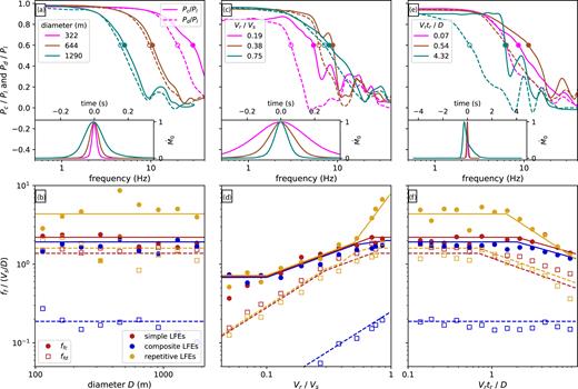
$(a, c, e) Coherent power fractions Pc/Pl (solid lines) and Pd/Pl (dashed lines) as a function of frequency for various groups of synthetic LFEs. Circles mark the coherence falloff frequencies: when Pc/Pl or Pd/Pl falls below 0.6. Inset panels show the moment rate functions averaged over LFEs in each group. Colour indicates diameter (panel a), rupture velocity (panel c), and rise time (panel e). (b, d, f) Normalized coherence falloff frequencies ffc/(Vs/D) (filled circles) and ffd/(Vs/D) (open squares) as a function of the LFE properties. Colour indicates the type of LFE rupture. Solid and dashed lines indicate visually estimated approximations of the numerically identified ffc and ffd to be used in our interpretations. In panels a, b, c and d, tr = 0.27D/Vr. In panels a, b, e and f, Vr = 0.75Vs. In panels c and e, D = 456 m. In panels d and f, the values plotted are medians taken from synthetics with seven different diameters.$

Figure 5.

(a, c, e) Coherent power fractions P_c/P_l (solid lines) and P_d/P_l (dashed lines) as a function of frequency for various groups of synthetic LFEs. Circles mark the coherence falloff frequencies: when P_c/P_l or P_d/P_l falls below 0.6. Inset panels show the moment rate functions averaged over LFEs in each group. Colour indicates diameter (panel a), rupture velocity (panel c), and rise time (panel e). (b, d, f) Normalized coherence falloff frequencies f_fc/(V_s/D) (filled circles) and f_fd/(V_s/D) (open squares) as a function of the LFE properties. Colour indicates the type of LFE rupture. Solid and dashed lines indicate visually estimated approximations of the numerically identified f_fc and f_fd to be used in our interpretations. In panels a, b, c and d, t_r = 0.27D/V_r. In panels a, b, e and f, V_r = 0.75V_s. In panels c and e, D = 456 m. In panels d and f, the values plotted are medians taken from synthetics with seven different diameters.

Open in new tab Download slide

6.3 Coherence falloff frequencies as a function of D, V_r and t_r

6.3.1 Coherence falloff with diameter

As anticipated in Section 2, both P_d/P_l and P_c/P_l decrease at lower frequencies (longer periods) when the LFE diameters are larger (panel a). P_d/P_l falls off earlier when diameters are larger because larger diameters imply longer ruptures, which allow for complexity and inter-LFE variability at lower frequencies. P_c/P_l falls off earlier because larger diameters imply larger shifts in the source–station traveltime within the rupture area, and thus allow for interstation ASTF variability at lower frequencies. To examine the coherence falloff systematically, we identify the frequencies at which P_d/P_l and P_c/P_l first fall below 0.6. These falloff frequencies f_fd and f_fc are normalized by V_s/D and plotted as a function of LFE diameter D in Fig. 5(b). In the simple LFE simulations in Fig. 5(b), which have V_r/V_s = 0.75 and t_r = 0.27R/V_r, f_fd is roughly 1.4V_s/D (open red squares and dashed red line), and f_fc is roughly 2.2V_s/D (filled red circles and solid red line).

6.3.2 Coherence falloff with rupture velocity

The direct coherence falloff frequency f_fd decreases relative to V_s/D if LFE rupture velocities are reduced, as shown Figs 5(c) and (d). Note that when we plot f_fd/(V_s/D) and f_fc/(V_s/D) in Figs 5(d) and (f), we take the median of estimates computed for seven groups of LFEs, with different diameters, in order to reduce the scatter. The decrease of f_fd/(V_s/D) with decreasing rupture velocities arises because lower rupture velocities allow for longer ruptures and therefore more complexity and interevent variability at lower frequencies. The LFEs’ heterogeneous slip distributions give rise to source time functions that differ among events at all periods shorter than the rupture duration, which scales as D/V_r in simulations of simple LFEs. The direct coherence falloff frequency f_fd thus scales inversely with the durations of these ruptures, with value around 2.8V_r/D when V_r < 0.4V_s, though it decreases relative to V_r/D for rupture velocities larger than 0.8V_s (red dashed line in Fig. 5d).

The interstation coherence falloff frequency f_fc depends more weakly on rupture velocity V_r. f_fc increases from 0.7 to 2.2V_s/D as V_r increases from 0.05 to 1V_s (filled red circles and solid red line in Fig. 5d). P_c/P_l depends only weakly on V_r because P_c/P_l measures how much the ASTFs vary among stations, not among events. The interstation ASTF variability depends primarily on the S-wave traveltime across the source region, which scales with D/V_s, not D/V_r. The V_r dependence that does exist likely results from the simpler ASTF pulses associated with higher rupture velocities. As V_r approaches V_s, the ASTFs tend towards single pulses, and interstation complexity is harder to distinguish.

6.3.3 Coherence falloff with rise time

Both f_fd and f_fc vary minimally in response to modest changes in the rise time t_r of slip at each point in the rupture, especially when t_r is less than D/V_r (Figs 5 c and f). In our implementation, we have assumed a spatially uniform rise time for each LFE. As a result, changing the rise time is roughly equivalent to convolving all of an LFE’s ASTFs by a single function, and such a convolution has little effect on the inter-ASTF coherence. We do allow roughly 10 |$\hbox{ per cent}$| variability in rise time and rupture velocity among the LFEs in each group. These rise time differences, coupled with the increased complexity visible in longer-duration ruptures, are likely responsible for the reduced coherence falloff frequencies that become apparent once t_r exceeds 1 to 2D/V_r (red symbols and lines in Fig. 5d).

6.3.4 LFE durations

Increasing the rise time does increase LFE duration. To estimate an average duration for each group of 100 synthetic LFEs, we first extract the source time functions for the individual LFEs. We shift these source time functions using the time shifts estimated via cross-correlation when constructing the waveform template. Then we sum the source time functions to obtain an average source time function, or moment rate function. Finally, to obtain a single number that we can compare across simulations with a range of parameters, we define a 70 |$\hbox{ per cent}$| LFE duration: the length of the time interval that contains the central 70 |$\hbox{ per cent}$| of the moment for the average moment rate function.

We find that in our simple LFEs, these 70 |$\hbox{ per cent}$| durations are between 0.29 and 0.31D/V_r when the rise time t_r is 0.27D/V_r. The durations increase as t_r is increased, and tend toward 0.28t_r once t_r gets significantly longer than D/V_r.

LFE durations are shorter in synthetic ruptures that nucleate near the rupture centers. For our repetitive LFEs, which we assume nucleate within 0.1D of their center points, durations are 0.25 to 0.28D/V_r when t_r is 0.27D/V_r. LFE durations are longer in synthetic ruptures that nucleate near the rupture edges. The durations are between 0.35 and 0.37D/V_r when nucleation locations are within 0.1D of the rupture edge. The durations of composite LFE ruptures are determined by the number and timing of subevents. The presented LFEs, containing five subevents, have durations between 3 and 3.3D/V_r.

6.3.5 Composite LFEs

The composite LFEs, with their long, complex ruptures, have lower direct coherence P_d/P_l than the simple LFEs. The direct coherence falloff frequency f_fd is around 0.25V_r/D for all simulated events (open blue squares and dashed lines in Figs 5b, d and f). On the other hand, the composite and simple LFEs have similar interstation coherence P_c/P_l and similar interstation falloff frequencies f_fc (filled blue circles and solid blue line). As for the simple ruptures, the composite LFEs’ P_c/P_l and f_fc depend primarily on D/V_s: on how much the source–station traveltime can shift peaks in the source time functions.

6.3.6 Repetitive LFEs

Repetitive LFEs can have significantly higher coherence and falloff frequencies than simple or composite events, at least when the rupture velocity is larger than about 0.5V_s. As described in Section 6.1, the repetitive LFEs simulated in each group have similar slip distributions, and they all nucleate near the rupture center, so they have similar ASTFs and similar waveforms. This similarity explains the increase in P_d/P_l, but the increase in P_c/P_l is surprising at first glance, as P_c/P_l measures similarity across stations, not across events. The high P_c/P_l arises because the cross-spectra calculation that goes into P_c (eq. 4) is designed to remove complexity associated with the path effects, and it identifies as ‘path effect’ any component of the source–path convolution (eq. 3) that is common to all events. If the ASTFs are the same for all events, the P_c calculation cannot distinguish interstation ASTF variations from station-dependent Green’s functions, so ASTF variations are attributed to path effects, and P_c/P_l is high when LFEs are highly repetitive. The falloff frequencies f_fc can increase by as much as factor of 6 when V_r > 0.8V_s.

We note, however, that this factor of 6 increase in f_fc is just one plausible value. Here we have assumed that two-thirds of the LFE moment came from a repetitive component of the rupture, but higher or lower coherence could be achieved by assuming that more or less of the moment came from the repetitive component. We also note that the high coherence arises only when the rupture nucleation location is consistent from event to event. The falloff frequencies f_fc remain low if only 75 |$\hbox{ per cent}$| of the repetitive LFEs nucleate at the SE rupture edge and the other 25 |$\hbox{ per cent}$| nucleate on the NW edge (Fig. S24).

6.3.7 Coherence variation with station distribution

In all of the synthetic ruptures described above, we use the station distribution and LFE location appropriate for family 37140, because using this station distribution allows us to directly compare the synthetics with the data. Note that most of the stations are located southeast of the LFEs, so the seismic waves’ takeoff angles and thus the LFEs’ ASTFs are more similar among these stations than they would be among stations were located at a wider range of azimuths. We find that P_d/P_l and P_c/P_l decreases at frequencies that are 10–20 |$\hbox{ per cent}$|lower when we assign the recording stations to random azimuths (Figs S21 and S22). Simply reducing the number of stations creates no such coherence reduction, however. The coherent frequencies change minimally if we pick subsets of the stations for each computation, to mimic the varying data availability and noise level (Fig. S20).

7 INTERPRETATION OF LFE COHERENCE

We may now use our synthetic results to interpret the coherence obtained for the Parkfield LFE families, which show direct coherence P_d/P_l > 0.6 out to 4–5 Hz and interstation coherence P_c/P_l > 0.6 out to 8–16.5 Hz.

7.1 LFE location distribution

First, we note that the observed high-frequency coherence implies that LFEs within each family are strongly clustered in space. If LFEs were distributed over a wide range of locations, traveltimes from the LFE centroids to the recording stations would vary widely from event to event. But in our analysis, we allow only the origin time to be realigned from event to event. Any interstation time shifts produced by varying LFE locations should show up in our results as a decrease in coherence.

To determine the maximum location variation allowed by the observations, we recompute coherence values after artificially shifting the LFE locations by various amounts. We pick location shifts for each LFE in family 37140, drawing from bivariate normal distributions with 100-m to 1-km standard deviations along strike and depth. We use the IASP91 velocity model and TauP to compute the arrival time change for the stations observing each LFE (Kennett & Engdahl 1991; Crotwell et al.1999). We subtract the median arrival time change from these values, shift the seismograms by the station-dependent remainders, and compute the coherent power fractions. The family-averaged results are shown in Figs 6 and S15-s17. We find that the interstation coherent fraction P_c/P_l obtained at 11 Hz is reduced by 40 |$\hbox{ per cent}$| even for location shifts with just 250-m standard deviation (Fig. 6). The >0.6 11-Hz coherence values obtained for the median family thus imply that LFEs in each family are strongly clustered, with standard deviation in their locations typically smaller than 250 m.

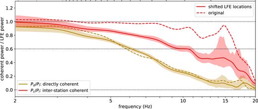
$Solid lines and shading: coherent power fractions for family 37140, as in Fig. 4(b), but computed after shifting the LFE locations by random amounts with 250-m standard deviations along strike and along depth. Dashed lines: original Pd/Pl and Pc/Pl, without location shifts, reproduced from Fig. 4(b).$

Figure 6.

Solid lines and shading: coherent power fractions for family 37140, as in Fig. 4(b), but computed after shifting the LFE locations by random amounts with 250-m standard deviations along strike and along depth. Dashed lines: original P_d/P_l and P_c/P_l, without location shifts, reproduced from Fig. 4(b).

Open in new tab Download slide

The distribution of LFE locations within a family, when coupled with noise, is one way to explain all of the incoherence observed at higher frequencies in the data. It is possible that each individual LFE is approximately a point source—that each LFE ruptures a tiny patch within a sub-1-km asperity (Chestler & Creager 2017a).

7.2 Matching f_fc, f_fd and duration with simple ruptures: results

However, it is also possible that the finite rupture areas of individual LFEs contribute to the decrease in coherence at high frequencies. To determine the maximum rupture areas and rupture velocities allowed by the data, we compare the observed coherence falloff frequencies and durations with those obtained from synthetics of simple, non-repetitive ruptures.

First, we note that the interstation coherence P_c/P_l remains higher than 0.6 out to 8–16.5 Hz for the various families. The median P_c/P_l falloff frequency f_fc is 11 Hz, and families 37102 and 37140 have f_fc of 9 and 16.5 Hz, respectively. We will discuss families 37102 and 37140 in more detail because Thomas et al. (2016) estimated their LFEs’ durations, and so we will be able to estimate their rupture velocities. In the synthetics, f_fc is 0.7–2.2V_s/D for rupture velocities V_r between 0.05 and 1V_s (red solid line in Fig. 5d). If the shear wave velocity V_s is around 4 km s^–1 in the LFE area (Lin et al.2010), family 37102s 9-Hz f_fc implies an average diameter smaller than 300–1000 m, with smaller allowable diameters for slower rupture velocities. In Fig. 7(a), this range of allowable diameters is marked with blue diagonal hatching. The blue shading marks the diameters allowed for family 37140. Its >16-Hz f_fc implies diameters smaller than 180–550 m.

Figure 7.

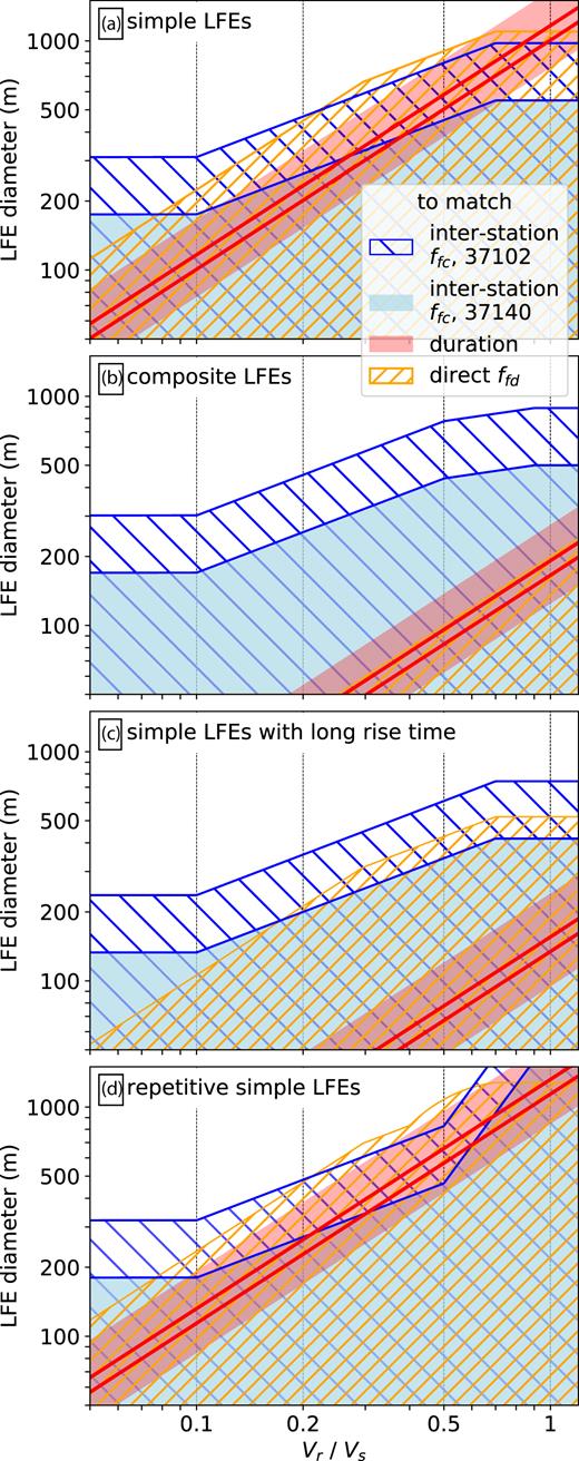
Hatching and shading: sets of diameters (y-axis) and rupture velocities (x-axis) that match each of the observations. Blue hatching and shading match f_fc for families 37102 and 37140, respectively. Yellow hatching matches the median f_fd for all families. Red shading matches the range of durations of Thomas et al. (2016), and the red lines match their best-fitting durations. The four panels are for four approaches to constructing the LFEs, as indicated by the text in the upper left.

Open in new tab Download slide

The orange diagonal hatching in Fig. 7(a) illustrates a further, albeit weaker, constraint on the LFEs’ diameters and rupture velocities: those obtained from the direct coherence P_d/P_l. P_d/P_l is higher than 0.6 out to 4–5 Hz for all seven LFE families, though it could be biased high or low by uncertainties in the LFE origin time alignment (see Appendix). In the synthetics, the P_d/P_l falloff frequency f_fd scales roughly with 1 divided by the rupture duration. f_fd ranges from 1.4 to 2.8V_r/D, or from 0.15 to 1.4V_s/D (blue dashed line in Fig. 5d). Coupling the synthetics with a 5-Hz observed f_fd constrains the LFE diameters to be less than 1100 m.

More important constraints on the LFE properties come from the LFE durations estimated by Thomas et al. (2016). Thomas et al. (2016) compared LFE stacks with nearby earthquakes’ waveforms and obtained best-fitting durations of 0.19 and 0.22s for LFEs in families 37140 and 37102, respectively. To get a sense of the duration uncertainty, we note that Thomas et al. (2016)’s best fits come from averaging over comparisons with 12 or 17 different local earthquakes, but they also present the durations obtained by the individual earthquake comparisons. Only one earthquake comparison gives a family 37140 duration smaller than 0.15 or larger than 0.22, and only one comparison gives a family 37102 duration smaller than 0.15 or larger than 0.3, so we use these values as uncertainty bounds.

To compare the durations to our synthetics, we note that 70 |$\hbox{ per cent}$| of the moment in the stacked synthetic LFEs accumulates within 0.29–0.31V_r/D. Thomas et al. (2016) modeled the LFE waveforms with a source time function shaped like a Hann window, which accumulates 70 |$\hbox{ per cent}$| of its moment within 40 |$\hbox{ per cent}$| of the total window length, so the 70 |$\hbox{ per cent}$| durations for families 37140 and 37102 are 0.060–0.087 and 0.060–0.12 s, respectively. We multiply these 70 |$\hbox{ per cent}$| durations by 1.4–2.8V_r to estimate LFE diameters and plot the results with red shading in Fig. 7(a). The lower and upper thick red lines mark the diameters expected for the best-fitting durations for families 37140 and 37102, respectively.

The diameters implied by the observed durations match those implied by family 37102s >9 Hz f_fc for a wide range of rupture velocities. The two sets of constraints overlap at least partially for all plotted V_r/V_s, and the interstation coherence constraint matches the median duration when V_r < V_s. According to these results, LFEs in family 37102 could be slow ruptures, with 200-m diameters and V_r = 0.2V_s. Or they could be relatively ‘normal’ earthquakes, with 800-m diameters and V_r = 0.8V_s. Note that changing the assumed shear wave velocity V_s would change the estimated diameters in Fig. 7, but not the V_r/V_s intersection ranges, as all of the plotted diameter constraints scale with 1/V_s.

Given the uncertainties in the data, the constraints on LFEs in family 37140 could also be matched with a range of rupture speeds. This family’s f_fc > 16 Hz constraint (blue shading in Fig. 7a) starts to intersects the edge of the duration constraints when V_r < 0.7V_s. Note, however, that the plotted 16-Hz constraint is already the 95 |$\hbox{ per cent}$| lower bound on f_fc, obtained from bootstrapping. The best-fitting f_fc is 16.5 Hz. Lower rupture speeds would match the data better. For instance, to match family 37140’s best-fitting duration (lower red line) and the constraint that f_fc ≳ 16 Hz (blue shading), the LFE rupture speeds should be less than 0.4V_s.

7.3 Matching f_fc, f_fd and duration with simple ruptures: Uncertainties

There are several uncertainties in the data and models that are not represented with the bootstrap-based uncertainty bounds. We consider how these would influence the rupture velocity estimates. For instance, one might imagine that all ruptures begin at the asperity edge and rupture unilaterally. In synthetics, groups of ruptures starting within 0.1D of the LFE edge have durations of 0.35 to 0.37D/V_r, longer than the 0.29–0.31D/V_r values estimated for events starting within 0.4D of the centre. Interpreting Thomas et al. (2016)'s durations via unilateral rupture would cause our duration-estimated diameters to decrease by about 20 |$\hbox{ per cent}$| moving the red lines in Fig. 7(a) down. However, synthetic ruptures starting from the edge also give f_fc values about 20 |$\hbox{ per cent}$| smaller than those starting closer to the center (Fig. S19). Changing both constraints thus moves both the red and blue lines down in Fig. 7(a), and leaves the range of allowable rupture velocities almost unchanged.

Other minor modifications to the rupture parameters appear to affect the f_fc constraints minimally. For instance, we observe little change in f_fc if we add a smooth tapered component to the heterogeneous slip distributions (Fig. S23) or if we limit the range of diameters within each group to a factor of 1.1 standard deviation (Fig. S25). However, we have not explored the entire range of rupture parameters. Perhaps we would obtain higher coherence if we made the slip distribution and temporal evolution smoother or slightly more repetitive, more similar to the repeater-like LFEs discussed in Sections 6.1 and 7.4.

Another scenario that seems unlikely but possible is that the 16.5-Hz f_fc obtained for family 37140 reflects random variability in the data or noise. This f_fc is significantly larger than the median f_fc for the seven families, which is just 11-Hz, and the synthetics in Fig. 5(b) do show tens of per cent variability in f_fc among LFE groups, simply as a result of random variations in the slip distributions. However, those synthetics use only 100 LFEs. Using several thousand should reduce the uncertainty. Further, bootstrapping events within each synthetic group gives a reasonable estimate of the variability among the groups. Bootstrapping the data in family 37140 gives 95 |$\hbox{ per cent}$| probability that f_fc > 16 Hz.

The other uncertainties in the data, along with potential variation in LFE location, would imply that the estimated 16.5-Hz f_fc is a lower bound on the true value, as discussed in Section 5 and appendix. Accounting for noise or variable LFE locations would push the allowable diameters and the blue shading in Fig. 7(a) down to lower values, making it harder to match the data with high rupture speeds. Given the uncertainties, we cannot exclude the possibility that these LFEs are simple ruptures with ‘typical’ earthquake rupture speeds around 0.7V_s. But we consider it more likely that the rupture velocities are lower than 0.7V_s (blue and red shading in Fig. 7a). The data are best matched by simple LFEs when rupture velocities are less than 0.4V_s (blue shading and red line).

7.4 Matching the data with modified LFE ruptures

It is also possible to match the data if we modify the LFE dynamics significantly: if LFEs are composite ruptures, ruptures with long rise times, or repetitive ruptures, as described in Section 6.1. Figs 7(b)–(d) illustrates the constraints obtained for some plausible rupture parameters.

Fig. 7(b) illustrates the constraints on diameters and rupture velocity if LFEs are composed of five subruptures distributed over an interval with duration 2.5D/V_r. Here the interstation coherence constraints (blue) are essentially unchanged, but the direct coherence and duration constraints imply smaller diameters.

Fig. 7(b) illustrates the constraints if LFEs have rise times equal to 5D/V_r. In these LFEs, rupture would progress to the asperity edge, and then the whole patch would continue slipping together.

Finally, Fig. 7(d) illustrates the constraints on D and V_r/V_s if LFEs are repetitive ruptures, which persistently nucleate in the same region, and which have two-thirds of their moment associated with a slip distribution that is consistent from event to event. With these repetitive ruptures, the 16-Hz f_fc of family 37140 can be matched even if the rupture diameters are larger.

A wide range of parameters could also match the data if LFE durations are actually reflections of local attenuation, not the LFE source dynamics (Gomberg et al.2012; Bostock et al.2017). In this case, the diameters estimated from the durations (red lines) are upper bounds, and the data can be matched by any combination of rupture velocity and diameter that plots below those bounds and within the f_fc (blue) and f_fd (yellow) constraints.

8 DISCUSSION

8.1 Implications for tremor asperities

Regardless of the individual LFE rupture dynamics, our observations of high-frequency coherence suggest that LFEs are clustered in patches less than 1 km across. As noted in the introduction, such clustering has also been inferred from careful analysis of LFE families in Cascadia (Sweet et al.2014; Chestler & Creager 2017a) and may be suggested by highly periodic LFE ruptures in Parkfield (Shelly 2010b). The clustering may suggest a role for material heterogeneity in controlling the occurrence of tremor. It is consistent with proposals that tremor’s LFEs rupture a collection of unstable asperities embedded in a larger, more stable region (Ando et al.2010, 2012; Nakata et al.2011; Ariyoshi et al.2012; Veedu & Barbot 2016; Luo & Ampuero 2017). Larger asperities may also exist, as patches of tremor are observed on scales of a few to tens of km. The larger tremor patches could represent groups of tremor asperities or regions more prone to distributed rapid slip (Shelly 2010b; Ghosh et al.2012; Armbruster et al.2014; Yabe & Ide 2014; Savard & Bostock 2015; Annoura et al.2016; Kano et al.2018). Alternatively, the large and small tremor patches could represent persistent slip patterns that have arisen on a simple, homogeneous fault. Such patterns are sometimes seen in models that lack heterogeneity in material properties (Horowitz & Ruina 1989; Langer et al.1996; Shaw & Rice 2000), though it remains to be assessed whether these models can produce clusters of tremor that persist over many slow slip cycles, as we observe in Parkfield.

The family-based clustering implied by our coherence estimates and by others’ LFE relocations (Sweet et al.2014; Chestler & Creager 2017a) suggests that cross-correlation based LFE families are more than an observational convenience (Shelly et al.2007; Brown et al.2008; Bostock et al.2012; Frank et al.2013; Kato 2017; Shelly 2017). The analysed families show sub-km LFE clustering even though some families are separated from identified neighboring families by a few to 5 km. The LFEs’ tendency to occur on these asperities lends further confidence to studies that have interpreted LFE repeat rates as indicators of the slip rate in a creeping area surrounding the more unstable LFE patches (Rubin & Armbruster 2013; Royer et al.2015; Lengliné et al.2017; Thomas et al.2018).

8.2 Implications for tremor physics

Given our observations and synthetics of LFE coherence as a function of rupture diameter, there are still several ways to explain the long, 0.2-s durations of Parkfield LFEs. First, it is possible that families 37102 and 37140’s LFEs are normal earthquakes with near-shear-wave rupture speeds. A 0.7V_s rupture speed is at the edge of the constraints for family 37140, but it can match the constraints on family 37102 well, and it may be worth noting that family 37140 shows exceptionally high coherence while Family 37102 has coherent power profiles that are more similar to the profiles of the other five families, for which we cannot estimate rupture velocities because we do not know their durations.

Further, 0.7V_s rupture velocities could match the data better if the LFEs are somewhat repetitive, with nucleation locations and slip distributions that persist from event to event. And a wide range of high rupture speeds could match the data if the 0.2-s durations we use are overestimates of the true durations, despite Thomas et al. (2016)’s careful empirical Green’s function analysis. The durations could be overestimated if a highly attenuating region is localized around the LFE patches, so that attenuation removes the high-frequency components of the LFE seismograms but has little effect on the seismograms of the reference earthquakes, which are located a few km away.

If LFEs do have durations of 0.2 s and rupture speeds up to 0.7V_s, they could have diameters up to 800 m. Uniform stress drop M_W 1 to 2 earthquakes with 800-m diameters would have stress drops of 0.3 to 9 kPa and average slips of 0.002-0.06 mm (Eshelby 1957; Shearer 2009). These moment and slip estimates are imprecise, and difficult to estimate because LFE locations are offset from local earthquakes, but we note that if the larger slip estimates are representative, almost all of the slip on the LFE patch could be seismic. Even 800-m-wide LFEs could accommodate most of the long-term slip on the LFE patch, which Thomas et al. (2016) estimated to be around 0.05 mm per event.

But while LFEs from both families can be matched by rupture velocities up to 0.7V_s, the data from family 37140 are better matched by LFEs with slower rupture speeds (<0.4V_s), long rise times, or a composite of subevents. Any of these scenarios would have interesting implications for the physics of LFE ruptures. For instance, rupture speeds around 0.4V_s, which can match the data for both families, would suggest that the LFEs’ radiation efficiency is around 0.5: that about half of the energy in LFEs is released via seismic wave generation, with the rest expended as fracture energy (e.g. Kostrov 1966; Eshelby 1969; Fossum & Freund 1975; Venkataraman & Kanamori 2004; Kanamori & Rivera 2006). Such low but significant radiation efficiency could mean that LFEs are exceptionally weak but otherwise normal earthquakes; LFEs may be driven by unstable frictional sliding, with slip rates limited by seismic wave radiation. Although 0.4V_s is lower than typical earthquake rupture speeds (McGuire 2004; Seekins & Boatwright 2010; Folesky et al.2016; Ye et al.2016; Melgar & Hayes 2017; Chounet et al.2018), such speeds are sometimes observed in earthquakes, especially in shallow tsunami earthquakes (e.g. Ide et al.1993; Ihmlé et al.1998; Venkataraman & Kanamori 2004; Bilek & Engdahl 2007; Polet & Kanamori 2009; Cesca et al.2011).

It is thus possible that LFEs are simply earthquakes driven by a frictional weakening process that is for some reason smaller in magnitude than the processes driving normal earthquakes. LFEs might nucleate ‘earlier’ than most earthquakes, at times when there is only a modest stress drop available to drive rupture. Or LFEs could nucleate on small unstable patches but then move quickly into regions that resist high slip speeds, perhaps because they are velocity-strengthening or allow for large off-fault deformation. Such acceleration-resisting regions have been suggested to limit the rupture velocities of tsunami earthquakes (e.g. Bilek & Lay 2002; Faulkner et al.2011a; Ma 2012). Off-fault deformation seems an appealing process to invoke for tremor because complex brittle and ductile deformation is observed at relevant depths (Fusseis et al.2006; Handy et al.2007; Collettini et al.2011; Fagereng et al.2014; Hayman & Lavier 2014; Angiboust et al.2015; Behr et al.2018; Webber et al.2018). It is even possible that each LFE is a collection of small brittle failures, rupturing small faults or veins (Fagereng et al.2014; Ujiie et al.2018). However, it remains unclear how or if that distributed ductile deformation would limit the rupture speeds of LFEs. Off-fault ductile deformation is also thought to accumulate in large earthquakes, which have near-shear-wave rupture speeds (DeDontney et al.2011; Dunham et al.2011; Roten et al.2017).

Another possibility is that LFEs do rupture at near-shear-wave speeds, but that the shear wave speed is significantly reduced in the LFE area because of lithological variations, fault zone damage, or high pore pressures (Audet et al.2009; Song et al.2009; Kato et al.2010; Fagereng & Diener 2011; Stefano et al.2011; Huang et al.2014). Fault damage zones are frequently observed at a range of depths (Shipton & Cowie 2001; Rowe et al.2009; Faulkner et al.2011b; Rempe et al.2013; Leclère et al.2015), and they sometimes show 30–50|$\hbox{ per cent}$| reductions in wavespeed, at least in shallow regions (Ben-Zion et al.2003; Cochran et al.2009; Lewis & Ben-Zion 2010; Yang et al.2014; Li et al.2016). It is difficult to fully assess a low-wavespeed region’s implications for our observations. The interstation coherence we observe depends on the seismic waves’ source–station traveltimes, and those times depend on which source–station paths are traveled. But in the simplest case, where LFE signals begin by traveling horizontally away from the fault, so that they move outside the fault zone before continuing to the surface, the traveltime variation we probe with interstation coherence would depend primarily on the higher wavespeed outside the fault zone. The higher wavespeeds could allow for the high-frequency interstation coherence we observe even though the lower wave speed inside the fault zone limits the rupture velocity and produces long-duration events.

On the other hand, it is possible that LFE rupture velocities are not limited by seismic wave radiation at all, but by a different fault zone rheology. We note that the results from family 37140 are best fit by simple LFE ruptures with V_r < 0.4V_s, and because of noise in the data, all of our coherence-constrained diameters and rupture speeds are upper bounds on the true values. So LFE rupture speeds could be much smaller: 0.2V_s, for example. Such slowly rupturing LFEs would release more than 80|$\hbox{ per cent}$| of their energy via fracture energy, making it unlikely that the energy dissipated via seismic wave radiation could limit the slip speeds. The low rupture velocities inferred for family 37140 could be telling us that LFE rupture dynamics are controlled by a different deformation mechanism than normal earthquakes—perhaps by the same speed-limiting rheology that controls slow slip events (e.g. Shibazaki & Iio 2003; Ide et al.2007; Shibazaki & Shimamoto 2007; Ide et al.2008; Aguiar et al.2009; Liu et al.2010; Segall et al.2010; Gao et al.2012; Hawthorne & Rubin 2013; Ide & Yabe 2014; Hawthorne & Bartlow 2018).

9 CONCLUSIONS

We have analysed interstation and interevent coherence between LFEs in seven families near Parkfield, CA. Our synthetic analysis shows that we can use interstation ASTF variations to estimate LFE location distributions or rupture areas. Our observations of LFE coherence imply that LFEs in each family are clustered in a small region, with standard deviation in their locations smaller than 250 m. Comparing the observed coherence with the coherence of synthetic LFE ruptures implies that LFE diameters are smaller than 500–1100 m, depending on the family. Coupling the diameter constraints with the LFE durations estimated by Thomas et al. (2016) for families 37102 and 37140 has allowed us to assess plausible rupture velocities. We could match the data for LFEs in family 37102 with a wide range of rupture models, including earthquake-like ruptures with rupture velocities V_r of 0.7–0.9 times the shear wave speed V_s. V_r = 0.7V_s can also match the data for family 37140, but only on the edge of the constraints. The data are better matched with lower rupture speeds V_r < 0.4V_s. Such low rupture speeds may indicate that LFEs are governed by a slow slip rheology, not by unstable frictional sliding. Alternatively, the data from both families of LFEs could be matched if LFEs rupture a fault zone with low shear wave speed, or if LFEs are repetitive fast ruptures, composite ruptures, or ruptures with long rise times. Our synthetics illustrate how the coherence and durations might differ among these rupture types, and thus how we might probe the physics of LFEs with future observations.

SUPPORTING INFORMATION

Figure S1. (a) Stacked templates for LFEs in Family 37140. Text indicates the network, station and channel. The grey bar indicates the time intervals used for the signal-to-noise check and in the power calculations. (b) Dark lines: Normalized amplitude spectra of the LFE intervals. Pastel lines: Normalized amplitude spectra of noise, from 3-second intervals starting 4 s before the LFE intervals. (c) Ratio of the LFE amplitude to the noise amplitude. The horizontal grey bar indicates signal amplitude we require to use a given template, as averaged over the marked frequency range.

Figure S2. As in Fig. S1, but for LFEs in family 37102.

Figure S3. As in Fig. S1, but for LFEs in family 9707.

Figure S4. As in Fig. S1, but for LFEs in family 77401.

Figure S5. As in Fig. S1, but for LFEs in family 27270.

Figure S6. As in Fig. S1, but for LFEs in family 45688.

Figure S7. As in Fig. S1, but for LFEs in family 70316.

Figure S8. Coherent and total power for family 37140. Markings are as in Figs 4(a) and (b).

Figure S9. Coherent and total power for family 37102. Markings are as in Figs 4(a) and (b).

Figure S10. Coherent and total power for family 9707. Markings are as in Figs 4(a) and (b).

Figure S11. Coherent and total power for family 77401. Markings are as in Figs 4(a) and (b).

Figure S12. Coherent and total power for family 27270. Markings are as in Figs 4(a) and (b).

Figure S13. Coherent and total power for family 45688. Markings are as in Figs 4(a) and (b).

Figure S14. Coherent and total power for family 70316. Markings are as in Figs 4(a) and (b).

Figure S15. Coherent and total power for family 37140, for 1-km standard deviation shifts.

Figure S16. Coherent and total power for family 37140, for 0.75-km standard deviation shifts.

Figure S17. Coherent and total power for family 37140, for 0.25-km standard deviation shifts.

Figure S18. As in Fig. 5, but using 500 LFEs in each group. Unlike in Fig. 5, values in panels d and f are not averaged over a range of diameters.

Figure S19. As in Fig. 5, but here the simple LFEs (red circles and squares) are required to start within 0.1D of the rupture edge.

Figure S20. As in Fig. 5, but here the simple LFEs (red circles and squares) are computed with a random subset of 5 stations, not with all the stations available for family 37140.

Figure S21. As in Fig. 5, but here when the simple LFEs (red circles and squares) are computed, we assign the observing stations to random azimuths between 0 and 360°. We retain the takeoff angles for the stations recording family 37140 LFEs, however.

Figure S22. As in Fig. 5, but here the simple LFEs (red circles and squares) are required to start within 0.1D of the rupture edge.

Figure S23. As in Fig. 5, but here the simple LFEs (red circles and squares) are computed with slip distributions that are offset from zero before computation.

Figure S24. As in Fig. 5, but here the repeating LFEs (yellow circles and squares) are computed with different directivity.

Figure S25. As in Fig. 5, but the radii are chosen from lognormal distributions with factor of 1.1 standard deviation instead of factor of 1.3 standard deviation.

Figure S26. As in Fig. 5, but here the Greens functions are not tapered white noise, but are instead taken to be the seismograms of a local earthquake that occurred 5 km away from the LFEs in family 37140.

Please note: Oxford University Press is not responsible for the content or functionality of any supporting materials supplied by the authors. Any queries (other than missing material) should be directed to the corresponding author for the article.

ACKNOWLEDGEMENTS

We used seismic waveform data from the Berkeley Parkfield High Resolution Seismic Network (HRSN), provided via the Northern California Earthquake Data Center and the Berkeley Seismological Laboratory (doi: 10.7932/NCEDC), as well as seismic waveform data from the Plate Boundary Observatory (PBO) borehole seismic network, operated by UNAVCO and funded by NSF grant EAR-0732947. The PBO data was obtained via IRIS. The fault traces shown in Fig. 2 were obtained from the USGS and California Geological Survey fault and fold database, accessed from http://earthquake.usgs.gov/hazards/qfaults in 2016. We are grateful to David Shelly for providing an earlier version of his Parkfield LFE catalog. We thank the editor and reviewers for comments that improved the paper.

REFERENCES

Aguiar

A.C.

,

Melbourne

T.I.

,

Scrivner

C.W.

,

2009

.

Moment release rate of Cascadia tremor constrained by GPS

,

J. geophys. Res.

,

114

,

B00A05

.

Ando

R.

,

Nakata

R.

,

Hori

T.

,

2010

.

A slip pulse model with fault heterogeneity for low-frequency earthquakes and tremor along plate interfaces

,

Geophys. Res. Lett.

,

37

,

L10310

.

Google Scholar

OpenURL Placeholder Text

WorldCat

Ando

R.

,

Takeda

N.

,

Yamashita

T.

,

2012

.

Propagation dynamics of seismic and aseismic slip governed by fault heterogeneity and Newtonian rheology

,

J. geophys. Res.

,

117

(

B11

),

B11308

.

Angiboust

S.

,

Kirsch

J.

,

Oncken

O.

,

Glodny

J.

,

Monié

P.

,

Rybacki

E.

,

2015

.

Probing the transition between seismically coupled and decoupled segments along an ancient subduction interface

,

Geochem., Geophys., Geosyst.

,

16

(

6

),

1905

–

1922

.

Annoura

S.

,

Obara

K.

,

Maeda

T.

,

2016

.

Total energy of deep low-frequency tremor in the Nankai subduction zone, southwest Japan

,

Geophys. Res. Lett.

,

43

(

6

),

2562

–

2567

.

Ariyoshi

K.

,

Hori

T.

,

Ampuero

J.-P.

,

Kaneda

Y.

,

Matsuzawa

T.

,

Hino

R.

,

Hasegawa

A.

,

2009

.

Influence of interaction between small asperities on various types of slow earthquakes in a 3-D simulation for a subduction plate boundary

,

Gondwana Res.

,

16

(

3-4

),

534

–

544

.

Ariyoshi

K.

,

Matsuzawa

T.

,

Ampuero

J.-P.

,

Nakata

R.

,

Hori

T.

,

Kaneda

Y.

,

Hino

R.

,

Hasegawa

A.

,

2012

.

Migration process of very low-frequency events based on a chain-reaction model and its application to the detection of preseismic slip for megathrust earthquakes

,

Earth Planets Space

,

64

(

8

),

693

–

702

.

Armbruster

J.G.

,

Kim

W.-Y.

,

Rubin

A.M.

,

2014

.

Accurate tremor locations from coherent S and P waves

,

J. geophys. Res.

,

119

(

6

),

5000

–

5013

.

Audet

P.

,

Schaeffer

A.J.

,

2018

.

Fluid pressure and shear zone development over the locked to slow slip region in Cascadia

,

Sci. Adv.

,

4

(

3

),

eaar2982

.

Audet

P.

,

Bostock

M.G.

,

Christensen

N.I.

,

Peacock

S.M.

,

2009

.

Seismic evidence for overpressured subducted oceanic crust and megathrust fault sealing

,

Nature

,

457

,

76

–

78

.

Baltay

A.

,

Prieto

G.

,

Beroza

G.C.

,

2010

.

Radiated seismic energy from coda measurements and no scaling in apparent stress with seismic moment

,

J. geophys. Res.

,

115

,

B08314

.

Behr

W.M.

,

Kotowski

A.J.

,

Ashley

K.T.

,

2018

.

Dehydration-induced rheological heterogeneity and the deep tremor source in warm subduction zones

,

Geology

,

46

(

5

),

475

–

478

.

Bell

R.

,

Sutherland

R.

,

Barker

D.H.N.

,

Henrys

S.

,

Bannister

S.

,

Wallace

L.

,

Beavan

J.

,

2010

.

Seismic reflection character of the Hikurangi subduction interface, New Zealand, in the region of repeated Gisborne slow slip events

,

Geophys. J. Int.

,

180

(

1

),

34

–

48

.

Ben-Zion

Y.

et al. ,

2003

.

A shallow fault-zone structure illuminated by trapped waves in the Karadere–Duzce branch of the North Anatolian Fault, western Turkey

,

Geophys. J. Int.

,

152

(

3

),

699

–

717

.

Bilek

S.L.

,

Engdahl

E.R.

,

2007

.

Rupture characterization and aftershock relocations for the 1994 and 2006 tsunami earthquakes in the Java subduction zone

,

Geophys. Res. Lett.

,

34

(

20

).

Google Scholar

OpenURL Placeholder Text

WorldCat

Bilek

S.L.

,

Lay

T.

,

2002

.

Tsunami earthquakes possibly widespread manifestations of frictional conditional stability

,

Geophys. Res. Lett.

,

29

(

14

),

1

–

4

.

Bostock

M.G.

,

Royer

A.A.

,

Hearn

E.H.

,

Peacock

S.M.

,

2012

.

Low frequency earthquakes below southern Vancouver Island

,

Geochem., Geophys., Geosyst.

,

13

(

11

),

Q11007

.

Bostock

M.G.

,

Thomas

A.M.

,

Savard

G.

,

Chuang

L.

,

Rubin

A.M.

,

2015

.

Magnitudes and moment-duration scaling of low-frequency earthquakes beneath southern Vancouver Island

,

J. geophys. Res.

,

120

(

9

),

6329

–

6350

.

Bostock

M.G.

,

Thomas

A.M.

,

Rubin

A.M.

,

Christensen

N.I.

,

2017

.

On corner frequencies, attenuation, and low-frequency earthquakes

,

J. geophys. Res.

,

122

(

1

),

543

–

557

.

Brown

J.R.

,

Beroza

G.C.

,

Shelly

D.R.

,

2008

.

An autocorrelation method to detect low frequency earthquakes within tremor

,

Geophys. Res. Lett.

,

35

(

16

),

L16305

.

Brown

J.R.

et al. ,

2009

.

Deep low-frequency earthquakes in tremor localize to the plate interface in multiple subduction zones

,

Geophys. Res. Lett.

,

36

,

L19306

.

Cesca

S.

,

Dahm

T.

,

Juretzek

C.

,

Kühn

D.

,

2011

.

Rupture process of the 2001 May 7 Mw 4.3 Ekofisk induced earthquake

,

Geophys. J. Int.

,

187

(

1

),

407

–

413

.

Chamberlain

C.J.

,

Shelly

D.R.

,

Townend

J.

,

Stern

T.A.

,

2014

.

Low-frequency earthquakes reveal punctuated slow slip on the deep extent of the Alpine Fault, New Zealand

,

Geochem., Geophys., Geosyst.

,

15

(

7

),

2984

–

2999

.

Chestler

S.R.

,

Creager

K.C.

,

2017a

.

Evidence for a scale-limited low-frequency earthquake source process

,

J. geophys. Res.

,

122

(

4

),

3099

–

3114

.

Chestler

S.R.

,

Creager

K.C.

,

2017b

.

A model for low-frequency earthquake slip

,

Geochem., Geophys., Geosyst.

,

18

(

12

),

4690

–

4708

.

Chounet

A.

,

Vallée

M.

,

Causse

M.

,

Courboulex

F.

,

2018

.

Global catalog of earthquake rupture velocities shows anticorrelation between stress drop and rupture velocity

,

Tectonophysics

,

733

,

148

–

158

.

Cochran

E.S.

,

Li

Y.-G.

,

Shearer

P.M.

,

Barbot

S.

,

Fialko

Y.

,

Vidale

J.E.

,

2009

.

Seismic and geodetic evidence for extensive, long-lived fault damage zones

,

Geology

,

37

(

4

),

315

–

318

.

Collettini

C.

,

Niemeijer

A.

,

Viti

C.

,

Smith

S.A.

,

Marone

C.

,

2011

.

Fault structure, frictional properties and mixed-mode fault slip behavior

,

Earth planet. Sci. Lett.

,

311

(

3–4

),

316

–

327

.

Crotwell

H.P.

,

Owens

T.J.

,

Ritsema

J.

,

1999

.

The TauP toolkit: flexible seismic travel-time and ray-path utilities

,

Seism. Res. Lett.

,

70

(

2

),

154

–

160

.

DeDontney

N.

,

Templeton-Barrett

E.L.

,

Rice

J.R.

,

Dmowska

R.

,

2011

.

Influence of plastic deformation on bimaterial fault rupture directivity

,

J. geophys. Res.

,

116

(

B10

),

B10312

.

Dunham

E.M.

,

Belanger

D.

,

Cong

L.

,

Kozdon

J.E.

,

2011

.

Earthquake ruptures with strongly rate-weakening friction and off-fault plasticity, Part 1: planar faults

,

Bull. seism. Soc. Am.

,

101

(

5

),

2296

–

2307

.

Eshelby

J.D.

,

1957

.

The determination of the elastic field of an ellipsoidal inclusion, and related problems

,

Proc. R. Soc. Lond., A: Math. Phys. Sci.

,

241

(

1226

),

376

–

396

.

Eshelby

J.D.

,

1969

.

The elastic field of a crack extending non-uniformly under general anti-plane loading

,

J. Mech. Phys. Solids

,

17

(

3

),

177

–

199

.

Fagereng

Å.

,

Diener

J.F.A.

,

2011

.

San Andreas Fault tremor and retrograde metamorphism

,

Geophys. Res. Lett.

,

38

(

23

),

L23303

.

Fagereng

Å.

,

Hillary

G.W.B.

,

Diener

J.F.A.

,

2014

.

Brittle-viscous deformation, slow slip, and tremor

,

Geophys. Res. Lett.

,

41

(

12

),

4159

–

4167

.

Faulkner

D.R.

,

Mitchell

T.M.

,

Behnsen

J.

,

Hirose

T.

,

Shimamoto

T.

,

2011a

.

Stuck in the mud? Earthquake nucleation and propagation through accretionary forearcs

,

Geophys. Res. Lett.

,

38

(

18

),

L18303

.

Faulkner

D.R.

,

Mitchell

T.M.

,

Jensen

E.

,

Cembrano

J.

,

2011b

.

Scaling of fault damage zones with displacement and the implications for fault growth processes

,

J. geophys. Res.

,

116

,

B05403

.

Fletcher

J.B.

,

McGarr

A.

,

2011

.

Moments, magnitudes, and radiated energies of non-volcanic tremor near Cholame, CA, from ground motion spectra at UPSAR

,

Geophys. Res. Lett.

,

38

(

16

),

L16314

.

Folesky

J.

,

Kummerow

J.

,

Shapiro

S.A.

,

Häring

M.

,

Asanuma

H.

,

2016

.

Rupture directivity of fluid-induced microseismic events: observations from an enhanced geothermal system

,

J. geophys. Res.

,

121

(

11

),

8034

–

8047

.

Fossum

A.F.

,

Freund

L.B.

,

1975

.

Nonuniformly moving shear crack model of a shallow focus earthquake mechanism

,

J. geophys. Res.

,

80

(

23

),

3347

.

Frank

W.B.

,

Shapiro

N.M.

,

Kostoglodov

V.

,

Husker

A.L.

,

Campillo

M.

,

Payero

J.S.

,

Prieto

G.A.

,

2013

.

Low-frequency earthquakes in the Mexican Sweet Spot

,

Geophys. Res. Lett.

,

40

(

11

),

2661

–

2666

.

Frankel

A.

,

1991

.

High-frequency spectral falloff of earthquakes, fractal dimension of complex rupture, b value, and the scaling of strength on faults

,

J. geophys. Res.

,

96

,

6291

–

6302

.

Fry

B.

,

Chao

K.

,

Bannister

S.

,

Peng

Z.

,

Wallace

L.

,

2011

.

Deep tremor in New Zealand triggered by the 2010 Mw8.8 Chile earthquake

,

Geophys. Res. Lett.

,

38

(

15

),

L15306

.

Fusseis

F.

,

Handy

M.R.

,

Schrank

C.

,

2006

.

Networking of shear zones at the brittle-to-viscous transition (Cap de Creus, NE Spain)

,

J. Struct. Geol.

,

28

(

7

),

1228

–

1243

.

Gao

H.

,

Schmidt

D.A.

,

Weldon

R.J.

,

2012

.

Scaling relationships of source parameters for slow slip events

,

Bull. seism. Soc. Am.

,

102

(

1

),

352

–

360

.

Ghosh

A.

,

Vidale

J.E.

,

Creager

K.C.

,

2012

.

Tremor asperities in the transition zone control evolution of slow earthquakes

,

J. geophys. Res.

,

117

(

B10

),

B10301

.

Gomberg

J.

,

Creager

K.

,

Sweet

J.

,

Vidale

J.

,

Ghosh

A.

,

Hotovec

A.

,

2012

.

Earthquake spectra and near-source attenuation in the Cascadia subduction zone

,

J. geophys. Res.

,

117

(

B5

),

B05312

.

Got

J.-L.

,

Fréchet

J.

,

1993

.

Origins of amplitude variations in seismic doublets: Source or attenuation process?

.

Geophys. J. Int.

,

114

(

2

),

325

–

340

.

Handy

M.R.

,

Hirth

G.

,

Burgmann

R.

,

2007

.

Continental fault structure and rheology from the frictional-to-viscous transition downwards

, in

Tectonic Faults: Agents of Change on a Dynamic Earth (Dahlem Workshop 95, Berlin, January 2005)

, pp.

139

–

182

., eds

Handy

M.R.

,

Hirth

G.

,

Hovius

N.

,

MIT Press

.

Google Scholar

Google Preview

OpenURL Placeholder Text

WorldCat

Hawthorne

J.C.

,

Ampuero

J.-P.

,

2017

.

A phase coherence approach to identifying co-located earthquakes and tremor

,

Geophys. J. Int.

,

209

(

2

),

623

–

642

.

Google Scholar

OpenURL Placeholder Text

WorldCat

Hawthorne

J.C.

,

Bartlow

N.M.

,

2018

.

Observing and modeling the spectrum of a slow slip event

,

J. geophys. Res.

,

123

(

5

),

4243

–

4265

.

Hawthorne

J.C.

,

Rubin

A.M.

,

2013

.

Laterally propagating slow slip events in a rate and state friction model with a velocity-weakening to velocity-strengthening transition

,

J. geophys. Res.

,

118

(

7

),

3785

–

3808

.

Hayman

N.W.

,

Lavier

L.L.

,

2014

.

The geologic record of deep episodic tremor and slip

,

Geology

,

42

(

3

),

195

–

198

.

Herrero

A.

,

Bernard

P.

,

1994

.

A kinematic self-similar rupture process for earthquakes

,

Bull. seism. Soc. Am.

,

84

(

4

),

1216

–

1228

.

Google Scholar

OpenURL Placeholder Text

WorldCat

Horowitz

F.G.

,

Ruina

A.

,

1989

.

Slip patterns in a spatially homogeneous fault model

,

J. geophys. Res.

,

94

(

B8

),

10 279

–

10 298

.

Hough

S.E.

,

1997

.

Empirical Green’s function analysis: Taking the next step

,

J. geophys. Res.

,

102

,

5369

–

5384

.

Huang

Y.

,

Ampuero

J.-P.

,

Helmberger

D.V.

,

2014

.

Earthquake ruptures modulated by waves in damaged fault zones

,

J. geophys. Res.

,

119

(

4

),

3133

–

3154

.

Ide

S.

,

Yabe

S.

,

2014

.

Universality of slow earthquakes in the very low frequency band

,

Geophys. Res. Lett.

,

41

(

8

),

2786

–

2793

.

Ide

S.

,

Imamura

F.

,

Yoshida

Y.

,

Abe

K.

,

1993

.

Source characteristics of the Nicaraguan Tsunami Earthquake of September 2, 1992

,

Geophys. Res. Lett.

,

20

(

9

),

863

–

866

.

Ide

S.

,

Beroza

G.C.

,

Shelly

D.R.

,

Uchide

T.

,

2007

.

A scaling law for slow earthquakes

,

Nature

,

447

(

7140

),

76

–

79

.

Ide

S.

,

Imanishi

K.

,

Yoshida

Y.

,

Beroza

G.C.

,

Shelly

D.R.

,

2008

.

Bridging the gap between seismically and geodetically detected slow earthquakes

,

Geophys. Res. Lett.

,

35

(

10

),

L10305

.

Ihmlé

P.F.

,

Gomez

J.-M.

,

Heinrich

P.

,

Guibourg

S.

,

1998

.

The 1996 Peru tsunamigenic earthquake: broadband source process

,

Geophys. Res. Lett.

,

25

(

14

),

2691

–

2694

.

Kanamori

H.

,

Brodsky

E.E.

,

2004

.

The physics of earthquakes

,

Rep. Prog. Phys.

,

67

(

8

),

1429

–

1496

.

Kanamori

H.

,

Rivera

L.

,

2006

.

Energy partitioning during an earthquake

,

Wash. DC Am. Geophys. Un. Geophys. Monogr. Ser.

,

170

,

3

–

13

.

Google Scholar

OpenURL Placeholder Text

WorldCat

Kane

D.L.

,

Shearer

P.M.

,

Goertz-Allmann

B.P.

,

Vernon

F.L.

,

2013

.

Rupture directivity of small earthquakes at Parkfield

,

J. geophys. Res.

,

118

(

1

),

212

–

221

.

Kano

M.

,

Kato

A.

,

Ando

R.

,

Obara

K.

,

2018

.

Strength of tremor patches along deep transition zone of a megathrust

,

Scientific Reports

,

8

(

1

),

3655

.

Kato

A.

,

2017

.

Illuminating deep tremors along the Nankai subduction zone, Japan, by matched filter technique

, in

Proceedings of the JpGU-AGU Joint Meeting

, pp.

SSS04

–

02

.

Google Scholar

Google Preview

OpenURL Placeholder Text

WorldCat

Kato

A.

et al. ,

2010

.

Variations of fluid pressure within the subducting oceanic crust and slow earthquakes

,

Geophys. Res. Lett.

,

37

,

L14310

.

Google Scholar

OpenURL Placeholder Text

WorldCat

Kennett

B.L.N.

,

Engdahl

E.R.

,

1991

.

Traveltimes for global earthquake location and phase identification

,

Geophys. J. Int.

,

105

(

2

),

429

–

465

.

Kitajima

H.

,

Saffer

D.M.

,

2012

.

Elevated pore pressure and anomalously low stress in regions of low frequency earthquakes along the Nankai Trough subduction megathrust

,

Geophys. Res. Lett.

,

39

(

23

),

L23301

.

Kostrov

B.V.

,

1966

.

Unsteady propagation of longitudinal shear cracks

,

J. Appl. Math. Mech.

,

30

(

6

),

1241

–

1248

.

Kwiatek

G.

,

Plenkers

K.

,

Dresen

G.

,

Group

J.R.

,

2011

.

Source parameters of picoseismicity recorded at Mponeng deep gold mine, South Africa: implications for scaling relations

,

Bull. seism. Soc. Am.

,

101

(

6

),

2592

–

2608

.

Langer

J.S.

,

Carlson

J.M.

,

Myers

C.R.

,

Shaw

B.E.

,

1996

.

Slip complexity in dynamic models of earthquake faults

,

Proc. Natl. Acad. Sci.

,

93

(

9

),

3825

–

3829

.

Leclère

H.

,

Cappa

F.

,

Faulkner

D.

,

Fabbri

O.

,

Armitage

P.

,

Blake

O.

,

2015

.

Development and maintenance of fluid overpressures in crustal fault zones by elastic compaction and implications for earthquake swarms

,

J. geophys. Res.

,

120

(

6

),

4450

–

4473

.

Lengliné

O.

,

Got

J.-L.

,

2011

.

Rupture directivity of microearthquake sequences near Parkfield, California

,

Geophys. Res. Lett.

,

38

,

L08310

.

Lengliné

O.

,

Frank

W.B.

,

Marsan

D.

,

Ampuero

J.P.

,

2017

.

Imbricated slip rate processes during slow slip transients imaged by low-frequency earthquakes

,

Earth planet. Sci. Lett.

,

476

,

122

–

131

.

Lewis

M.A.

,

Ben-Zion

Y.

,

2010

.

Diversity of fault zone damage and trapping structures in the Parkfield section of the San Andreas Fault from comprehensive analysis of near fault seismograms

,

Geophys. J. Int.

,

183

(

3

),

1579

–

1595

.

Li

Y.-G.

,

Catchings

R.D.

,

Goldman

M.R.

,

2016

.

Subsurface fault damage zone of the 2014 Mw 6.0 South Napa, California, earthquake viewed from fault-zone trapped waves

,

Bull. seism. Soc. Am.

,

106

(

6

),

2747

–

2763

.

Lin

G.

,

Thurber

C.H.

,

Zhang

H.

,

Hauksson

E.

,

Shearer

P.M.

,

Waldhauser

F.

,

Brocher

T.M.

,

Hardebeck

J.

,

2010

.

A California statewide three-dimensional seismic velocity model from both absolute and differential times

,

Bull. seism. Soc. Am.

,

100

(

1

),

225

–

240

.

Liu

L.

,

Gurnis

M.

,

Seton

M.

,

Saleeby

J.

,

Muller

R.D.

,

Jackson

J.M.

,

2010

.

The role of oceanic plateau subduction in the Laramide orogeny

,

Nat. Geosci.

,

3

(

5

),

353

–

357

.

Liu

Y.J.

,

Rice

J.R.

,

2005

.

Aseismic slip transients emerge spontaneously in three-dimensional rate and state modeling of subduction earthquake sequences

,

J. geophys. Res.

,

110

,

B08307

.

Google Scholar

OpenURL Placeholder Text

WorldCat

Liu

Y.J.

,

Rice

J.R.

,

2007

.

Spontaneous and triggered aseismic deformation transients in a subduction fault model

,

J. geophys. Res.

,

112

(

B9

),

B09404

.

Luo

Y.

,

Ampuero

J.-P.

,

2017

.

Tremor migration patterns and the collective behavior of deep asperities mediated by creep

,

EarthArXiv

.

Google Scholar

OpenURL Placeholder Text

WorldCat

Ma

S.

,

2012

.

A self-consistent mechanism for slow dynamic deformation and large tsunami generation for earthquakes in the shallow subduction zone

,

Geophys. Res. Lett.

,

39

(

11

),

L11310

.

Madariaga

R.

,

2007

.

Seismic source theory

, in

Treatise on Geophysics

, Vol.

4

:

Earthquake Seismology

, p.

6054

, eds

Kanamori

H.

,

Schubert

G.

,

Elsevier

, .

Google Scholar

Google Preview

OpenURL Placeholder Text

WorldCat

Maeda

T.

,

Obara

K.

,

2009

.

Spatiotemporal distribution of seismic energy radiation from low-frequency tremor in western Shikoku, Japan

,

J. geophys. Res.

,

114

,

B00A09

.

Mai

P.M.

,

Beroza

G.C.

,

2002

.

A spatial random field model to characterize complexity in earthquake slip

,

J. geophys. Res.

,

107

(

B11

),

2308

.

McGuire

J.J.

,

2004

.

Estimating finite source properties of small earthquake ruptures

,

Bull. seism. Soc. Am.

,

94

(

2

),

377

–

393

.

Melgar

D.

,

Hayes

G.P.

,

2017

.

Systematic observations of the slip pulse properties of large earthquake ruptures

,

Geophys. Res. Lett.

,

44

(

19

),

9691

–

9698

.

Mori

J.

,

Frankel

A.

,

1990

.

Source parameters for small events associated with the 1986 North Palm Springs, California, earthquake determined using empirical Green functions

,

Bull. seism. Soc. Am.

,

80

(

2

),

278

–

295

.

Google Scholar

OpenURL Placeholder Text

WorldCat

Mueller

C.S.

,

1985

.

Source pulse enhancement by deconvolution of an empirical Green’s function

,

Geophys. Res. Lett.

,

12

(

1

),

33

–

36

.

Nakata

R.

,

Ando

R.

,

Hori

T.

,

Ide

S.

,

2011

.

Generation mechanism of slow earthquakes: Numerical analysis based on a dynamic model with brittle-ductile mixed fault heterogeneity

,

J. geophys. Res.

,

116

(

B8

),

B08308

.

Nowack

R.L.

,

Bostock

M.G.

,

2013

.

Scattered waves from low-frequency earthquakes and plate boundary structure in northern Cascadia

,

Geophys. Res. Lett.

,

40

(

16

),

4238

–

4243

.

Obara

K.

,

2002

.

Nonvolcanic deep tremor associated with subduction in southwest Japan

,

Science

,

296

(

5573

),

1679

–

1681

.

Ohta

K.

,

Ide

S.

,

2011

.

Precise hypocenter distribution of deep low-frequency earthquakes and its relationship to the local geometry of the subducting plate in the Nankai subduction zone, Japan

,

J. geophys. Res.

,

116

,

B01308

.

Payero

J.S.

,

Kostoglodov

V.

,

Shapiro

N.

,

Mikumo

T.

,

Iglesias

A.

,

Perez-Campos

X.

,

Clayton

R.W.

,

2008

.

Nonvolcanic tremor observed in the Mexican subduction zone

,

Geophys. Res. Lett.

,

35

,

L07305

.

Perfettini

H.

,

Ampuero

J.P.

,

2008

.

Dynamics of a velocity strengthening fault region: Implications for slow earthquakes and postseismic slip

,

J. geophys. Res.

,

113

,

B09411

.

Peterson

C.L.

,

Christensen

D.H.

,

2009

.

Possible relationship between nonvolcanic tremor and the 1998–2001 slow slip event, south central Alaska

,

J. geophys. Res.

,

114

,

B06302

.

Polet

J.

,

Kanamori

H.

,

2009

.

Tsunami earthquakes

, in

Encyclopedia of Complexity and Systems Science

, pp.

9577

–

9592

.,

Springer

.

Google Scholar

Google Preview

OpenURL Placeholder Text

WorldCat

Poulet

T.

,

Veveakis

E.

,

Regenauer-Lieb

K.

,

Yuen

D.A.

,

2014

.

Thermo-poro-mechanics of chemically active creeping faults: 3. The role of serpentinite in episodic tremor and slip sequences, and transition to chaos

,

J. geophys. Res.

,

119

(

6

),

4606

–

4625

.

Prieto

G.A.

,

Shearer

P.M.

,

Vernon

F.L.

,

Kilb

D.

,

2004

.

Earthquake source scaling and self-similarity estimation from stacking P and S spectra

,

J. geophys. Res.

,

109

(

B8

),

B08310

.

Rempe

M.

,

Mitchell

T.

,

Renner

J.

,

Nippress

S.

,

Ben-Zion

Y.

,

Rockwell

T.

,

2013

.

Damage and seismic velocity structure of pulverized rocks near the San Andreas Fault

,

J. geophys. Res.

,

118

(

6

),

2813

–

2831

.

Rice

J.R.

,

1980

.

The mechanics of earthquake rupture

, in

Physics of the Earth’s Interior (Proc. Intl. School of Physics ”E. Fermi” Course 78)

, pp.

555

–

650

., eds

Dziewonski

A.M.

,

Boschi

E.

,

Italian Physical Society / North Holland Publishing Co

Google Scholar

Google Preview

OpenURL Placeholder Text

WorldCat

Rogers

G.

,

Dragert

H.

,

2003

.

Episodic tremor and slip on the Cascadia subduction zone: the chatter of silent slip

,

Science

,

300

(

5627

),

1942

–

1943

.

Roten

D.

,

Olsen

K.B.

,

Day

S.M.

,

2017

.

Off-fault deformations and shallow slip deficit from dynamic rupture simulations with fault zone plasticity

,

Geophys. Res. Lett.

,

44

(

15

),

7733

–

7742

.

Rowe

C.D.

,

Meneghini

F.

,

Moore

J.C.

,

2009

.

Fluid-rich damage zone of an ancient out-of-sequence thrust, Kodiak Islands, Alaska

,

Tectonics

,

28

,

1

–

20

.

Royer

A.A.

,

Bostock

M.G.

,

2014

.

A comparative study of low frequency earthquake templates in northern Cascadia

,

Earth planet. Sci. Lett.

,

402

,

247

–

256

.

Royer

A.A.

,

Thomas

A.M.

,

Bostock

M.G.

,

2015

.

Tidal modulation and triggering of low-frequency earthquakes in northern Cascadia

,

J. geophys. Res.

,

120

(

1

),

384

–

405

.

Rubin

A.M.

,

2008

.

Episodic slow slip events and rate-and-state friction

,

J. geophys. Res.

,

113

,

B11414

.

Rubin

A.M.

,

2009

.

Properties of Creep Fronts on Rate-and-State Faults

,

EOS Trans. Am. geophys. Un., Fall Meeting Suppl.

,

21

,

T21F

–

08

.

Google Scholar

OpenURL Placeholder Text

WorldCat

Rubin

A.M.

,

Armbruster

J.G.

,

2013

.

Imaging slow slip fronts in Cascadia with high precision cross-station tremor locations

,

Geochem., Geophys., Geosyst.

,

14

,

5371

–

5392

.

Rubin

A.M.

,

Bostock

M.G.

,

2017

.

What is this thing called tremor?

.

EOS Trans. Am. geophys. Un., Fall Meeting Suppl.

,

52

,

S52B

–

07

.

Google Scholar

Google Preview

OpenURL Placeholder Text

WorldCat

Rubinstein

J.L.

,

Shelly

D.R.

,

Ellsworth

W.L.

,

2009

.

Non-volcanic tremor: a window into the roots of fault zones

, in

New Frontiers in Integrated Solid Earth Sciences

, pp.

287

–

314

., eds

Negendank

J.

,

Cloetingh

S.

,

Springer

.

Google Scholar

Google Preview

OpenURL Placeholder Text

WorldCat

Saffer

D.M.

,

Wallace

L.M.

,

2015

.

The frictional, hydrologic, metamorphic and thermal habitat of shallow slow earthquakes

,

Nat. Geosci.

,

8

(

8

),

594

–

600

.

Savard

G.

,

Bostock

M.G.

,

2015

.

Detection and location of low-frequency earthquakes using cross-station correlation

,

Bull. seism. Soc. Am.

,

105

(

4

),

2128

–

2142

.

Seekins

L.C.

,

Boatwright

J.

,

2010

.

Rupture directivity of moderate earthquakes in northern California

,

Bull. seism. Soc. Am.

,

100

(

3

),

1107

–

1119

.

Segall

P.

,

Rubin

A.M.

,

Bradley

A.M.

,

Rice

J.R.

,

2010

.

Dilatant strengthening as a mechanism for slow slip events

,

J. geophys. Res.

,

115

,

B12305

.

Seno

T.

,

Yamasaki

T.

,

2003

.

Low-frequency tremors, intraslab and interplate earthquakes in Southwest Japan-from a viewpoint of slab dehydration

,

Geophys. Res. Lett.

,

30

(

22

),

1

–

4

.

Shaw

B.E.

,

Rice

J.R.

,

2000

.

Existence of continuum complexity in the elastodynamics of repeated fault ruptures

,

J. geophys. Res.

,

105

(

B10

),

23 791

–

23 810

.

Shearer

P.

,

2009

.

Introduction to Seismology

, 2nd edn,

Cambridge University Press

.

Google Scholar

Google Preview

OpenURL Placeholder Text

WorldCat

Shelly

D.R.

,

2010a

.

Migrating tremors illuminate complex deformation beneath the seismogenic San Andreas fault

,

Nature

,

463

(

7281

),

648

–

652

.

Shelly

D.R.

,

2010b

.

Periodic, chaotic, and doubled earthquake recurrence intervals on the deep San Andreas Fault

,

Science

,

328

(

5984

),

1385

–

1388

.

Shelly

D.R.

,

2017

.

A 15 year catalog of more than 1 million low-frequency earthquakes: Tracking tremor and slip along the deep San Andreas Fault

,

J. geophys. Res.

,

122

(

5

),

3739

–

3753

.

Shelly

D.R.

,

Hardebeck

J.L.

,

2010

.

Precise tremor source locations and amplitude variations along the lower-crustal central San Andreas Fault

,

Geophys. Res. Lett.

,

37

,

L14301

.

Shelly

D.R.

,

Beroza

G.C.

,

Ide

S.

,

Nakamula

S.

,

2006

.

Low-frequency earthquakes in Shikoku, Japan, and their relationship to episodic tremor and slip

,

Nature

,

442

(

7099

),

188

–

191

.

Shelly

D.R.

,

Beroza

G.C.

,

Ide

S.

,

2007

.

Non-volcanic tremor and low-frequency earthquake swarms

,

Nature

,

446

(

7133

),

305

–

307

.

Shelly

D.R.

,

Ellsworth

W.L.

,

Ryberg

T.

,

Haberland

C.

,

Fuis

G.S.

,

Murphy

J.

,

Nadeau

R.M.

,

Bürgmann

R.

,

2009

.

Precise location of San Andreas Fault tremors near Cholame, California using seismometer clusters: slip on the deep extension of the fault?

.

Geophys. Res. Lett.

,

36

(

1

),

L01303

.

Shibazaki

B.

,

Iio

Y.

,

2003

.

On the physical mechanism of silent slip events along the deeper part of the seismogenic zone

,

Geophys. Res. Lett.

,

30

(

9

),

1

–

4

.

Shibazaki

B.

,

Shimamoto

T.

,

2007

.

Modelling of short-interval silent slip events in deeper subduction interfaces considering the frictional properties at the unstable-stable transition regime

,

Geophys. J. Int.

,

171

(

1

),

191

–

205

.

Shipton

Z.K.

,

Cowie

P.A.

,

2001

.

Damage zone and slip-surface evolution over μm to km scales in high-porosity Navajo sandstone, Utah

,

J. Struct. Geol.

,

23

(

12

),

1825

–

1844

.

Skarbek

R.M.

,

Rempel

A.W.

,

Schmidt

D.A.

,

2012

.

Geologic heterogeneity can produce aseismic slip transients

,

Geophys. Res. Lett.

,

39

(

21

),

L21306

.

Song

T.-R.A.

,

Helmberger

D.V.

,

Brudzinski

M.R.

,

Clayton

R.W.

,

Davis

P.

,

Perez-Campos

X.

,

Singh

S.K.

,

2009

.

Subducting slab ultra-slow velocity layer coincident with silent earthquakes in southern Mexico

,

Science

,

324

(

5926

),

502

–

506

.

Stefano

R.D.

,

Chiarabba

C.

,

Chiaraluce

L.

,

Cocco

M.

,

Gori

P.D.

,

Piccinini

D.

,

Valoroso

L.

,

2011

.

Fault zone properties affecting the rupture evolution of the 2009 (Mw 6.1) L’Aquila earthquake (central Italy): insights from seismic tomography

,

Geophys. Res. Lett.

,

38

,

L10310

.

Sweet

J.R.

,

Creager

K.C.

,

Houston

H.

,

2014

.

A family of repeating low-frequency earthquakes at the downdip edge of tremor and slip

,

Geochem., Geophys., Geosyst.

,

15

(

9

),

3713

–

3721

.

Taira

T.

,

Dreger

D.S.

,

Nadeau

R.M.

,

2015

.

Rupture process for micro-earthquakes inferred from borehole seismic recordings

,

Int. J. Earth Sci.

,

104

(

6

),

1499

–

1510

.

Thomas

A.M.

,

Beroza

G.C.

,

Shelly

D.R.

,

2016

.

Constraints on the source parameters of low-frequency earthquakes on the San Andreas Fault

,

Geophys. Res. Lett.

,

43

(

4

),

1464

–

1471

.

Thomas

A.M.

,

Beeler

N.M.

,

Bletery

Q.

,

Burgmann

R.

,

Shelly

D.R.

,

2018

.

Using low-frequency earthquake families on the San Andreas Fault as deep creepmeters

,

J. geophys. Res.

,

123

(

1

),

457

–

475

.

Thomson

D.J.

,

1982

.

Spectrum estimation and harmonic analysis

,

Proc. IEEE

,

70

(

9

),

1055

–

1096

.

Tinti

E.

,

Fukuyama

E.

,

Piatanesi

A.

,

Cocco

M.

,

2005

.

A kinematic source-time function compatible with earthquake dynamics

,

Bull. seism. Soc. Am.

,

95

(

4

),

1211

–

1223

.

Uchide

T.

,

Shearer

P.M.

,

Imanishi

K.

,

2014

.

Stress drop variations among small earthquakes before the 2011 Tohoku-oki, Japan, earthquake and implications for the main shock

,

J. geophys. Res.

,

119

(

9

),

7164

–

7174

.

Ujiie

K.

,

Saishu

H.

,

Fagereng

Å.

,

Nishiyama

N.

,

Otsubo

M.

,

Masuyama

H.

,

Kagi

H.

,

2018

.

An explanation of episodic tremor and slow slip constrained by crack-seal veins and viscous shear in subduction mélange

,

Geophys. Res. Lett.

,

45

,

5371

–

5379

.

van Avendonk

H.J.A.

,

Holbrook

W.S.

,

Lizarralde

D.

,

Mora

M.M.

,

Harder

S.

,

Bullock

A.D.

,

Alvarado

G.E.

,

Ramírez

C.J.

,

2010

.

Seismic evidence for fluids in fault zones on top of the subducting Cocos Plate beneath Costa Rica

,

Geophys. J. Int.

,

181

(

2

),

997

–

1016

.

Google Scholar

OpenURL Placeholder Text

WorldCat

Veedu

D.M.

,

Barbot

S.

,

2016

.

The Parkfield tremors reveal slow and fast ruptures on the same asperity

,

Nature

,

532

,

361

–

365

.

Velasco

A.A.

,

Ammon

C.J.

,

Lay

T.

,

1994

.

Empirical green function deconvolution of broadband surface waves: Rupture directivity of the 1992 Landers, California (Mw = 7.3), earthquake

,

Bull. seism. Soc. Am.

,

84

(

3

),

735

–

750

.

Google Scholar

OpenURL Placeholder Text

WorldCat

Venkataraman

A.

,

Kanamori

H.

,

2004

.

Observational constraints on the fracture energy of subduction zone earthquakes

,

J. geophys. Res.

,

109

(

B5

),

B05302

.

Veveakis

E.

,

Poulet

T.

,

Alevizos

S.

,

2014

.

Thermo-poro-mechanics of chemically active creeping faults: 2. Transient considerations

,

J. geophys. Res.

,

119

(

6

),

4583

–

4605

.

Waldhauser

F.

,

2009

.

Near-real-time double-difference event location using long-term seismic archives, with application to northern California

,

Bull. seism. Soc. Am.

,

99

(

5

),

2736

–

2748

.

Walter

J.I.

,

Schwartz

S.Y.

,

Protti

J.M.

,

Gonzalez

V.

,

2011

.

Persistent tremor within the northern Costa Rica seismogenic zone

,

Geophys. Res. Lett.

,

38

,

L01307

.

Wang

E.

,

Rubin

A.M.

,

2011

.

Rupture directivity of microearthquakes on the San Andreas Fault from spectral ratio inversion

,

Geophys. J. Int.

,

186

(

2

),

852

–

866

.

Watanabe

T.

,

Hiramatsu

Y.

,

Obara

K.

,

2007

.

Scaling relationship between the duration and the amplitude of non-volcanic deep low-frequency tremors

,

Geophys. Res. Lett.

,

34

(

7

),

L07305

.

Webber

S.

,

Ellis

S.

,

Fagereng

Å.

,

2018

.

“Virtual shear box” experiments of stress and slip cycling within a subduction interface mélange

,

Earth planet. Sci. Lett.

,

488

,

27

–

35

.

Wech

A.G.

,

Creager

K.C.

,

2007

.

Cascadia tremor polarization evidence for plate interface slip

,

Geophys. Res. Lett.

,

34

(

22

).

Google Scholar

OpenURL Placeholder Text

WorldCat

Yabe

S.

,

Ide

S.

,

2014

.

Spatial distribution of seismic energy rate of tectonic tremors in subduction zones

,

J. geophys. Res.

,

119

(

11

),

8171

–

8185

.

Yabe

S.

,

Ide

S.

,

2017

.

Slip-behavior transitions of a heterogeneous linear fault

,

J. geophys. Res.

,

122

(

1

),

387

–

410

.

Yabe

S.

,

Baltay

A.S.

,

Ide

S.

,

Beroza

G.C.

,

2014

.

Seismic-wave attenuation determined from tectonic tremor in multiple subduction zonesseismic-wave attenuation determined from tectonic tremor in multiple subduction zones

,

Bull. seism. Soc. Am.

,

104

(

4

),

2043

–

2059

.

Yang

H.

,

Li

Z.

,

Peng

Z.

,

Ben-Zion

Y.

,

Vernon

F.

,

2014

.

Low-velocity zones along the San Jacinto Fault, Southern California, from body waves recorded in dense linear arrays

,

J. geophys. Res.

,

119

(

12

),

8976

–

8990

.

Ye

L.

,

Lay

T.

,

Kanamori

H.

,

Rivera

L.

,

2016

.

Rupture characteristics of major and great (Mw > = 7.0) megathrust earthquakes from 1990 to 2015: 1. Source parameter scaling relationships

,

J. geophys. Res.

,

121

(

2

),

826

–

844

.

Zhang

J.

,

Gerstoft

P.

,

Shearer

P.M.

,

Yao

H.

,

Vidale

J.E.

,

Houston

H.

,

Ghosh

A.

,

2011

.

Cascadia tremor spectra: low corner frequencies and earthquake-like high-frequency falloff

,

Geochem., Geophys., Geosyst.

,

12

(

10

),

Q10007

.

APPENDIX: DECOHERENCE FROM NOISE

Our coherence frequencies should probably be interpreted as lower bounds, as several sources of noise could reduce the observed P_d/P_l and P_c/P_l from their true values. First, decreased P_d/P_l and P_c/P_l could arise if a significant portion of the ‘noise’ comes from LFEs that are nearby but not in the family of interest. LFEs are clustered in space and time (e.g. Shelly 2010a; Bostock et al.2015) so the noise from other LFEs may be higher during the LFE window than during the noise window before it. We estimate the noise power P_n in a window that starts just 8 s before the LFE S arrival to minimize the potential difference, but we cannot account for sub-8 s clustering. Note that in principle our noise window could include some of the P arrival. However, we find the P arrival is too late and too small to significantly affect the P_n estimates. Truncating the noise waveforms before the P arrivals and reprocessing changes our results negligibly.

Decreased P_d/P_l and P_c/P_l could also result from noise in the template LFEs. The template signals start to become poorly resolved at frequencies higher than 15 Hz, so it is difficult to calculate robust powers at those frequencies. In addition, decreased P_d/P_l and P_c/P_l could arise if the path effect varies spatially within the families’ source region, so that the template and individual LFEs have different path effects.

Finally, decreased or increased P_d/P_l could result from uncertainty in the LFE origin time. To accurately calculate direct coherence at high frequencies, we need well aligned waveforms, so we recompute LFE origin times using 0.01-s precision. The realignment affects P_c/P_l negligibly but increases the frequencies with P_d/P_l > 0.6 by several Hz relative to results without recomputed origin time. One might worry that the increase in coherence comes from aligning the template with coherent noise rather than with LFE signal. However, we require at least five stations for the power estimates for each LFE, and we allow only one origin time shift per LFE. Assuming noise is random among stations, realigning with noise should increase P_d/P_l by less than 0.2.

The LFE detection approach of Shelly (2017) could also result in slightly increased coherence if noise contributes a part of the identified coherent signals. Finally, slightly increased coherence could result from our exclusion of signals with especially high noise. Note that the detected-facilitated increases in coherence are most likely to occur at low frequencies, around a few Hz, as these frequencies contribute most of the seismogram power involved in LFE selection and alignment.

There are no other obvious sources of artificially high coherence. Applying our processing to noise intervals rather than LFEs gives P_c/P_l and P_d/P_l of 0.01 or less.

This article is published and distributed under the terms of the Oxford University Press, Standard Journals Publication Model (https://dbpia.nl.go.kr/journals/pages/open_access/funder_policies/chorus/standard_publication_model)

Download all slides

Month:	Total Views:
October 2018	22
November 2018	18
December 2018	37
January 2019	25
February 2019	15
March 2019	23
April 2019	13
May 2019	36
June 2019	4
July 2019	9
August 2019	14
September 2019	16
October 2019	63
November 2019	33
December 2019	21
January 2020	53
February 2020	37
March 2020	29
April 2020	35
May 2020	12
June 2020	16
July 2020	20
August 2020	27
September 2020	5
October 2020	11
November 2020	17
December 2020	21
January 2021	14
February 2021	29
March 2021	16
April 2021	10
May 2021	17
June 2021	13
July 2021	20
August 2021	22
September 2021	10
October 2021	21
November 2021	27
December 2021	24
January 2022	18
February 2022	26
March 2022	22
April 2022	15
May 2022	26
June 2022	13
July 2022	19
August 2022	36
September 2022	35
October 2022	62
November 2022	27
December 2022	29
January 2023	16
February 2023	27
March 2023	26
April 2023	29
May 2023	9
June 2023	38
July 2023	6
August 2023	28
September 2023	13
October 2023	21
November 2023	23
December 2023	19
January 2024	15
February 2024	17
March 2024	24
April 2024	14
May 2024	46
June 2024	14
July 2024	24
August 2024	18
September 2024	11
October 2024	10
November 2024	19
December 2024	15
January 2025	23
February 2025	20
March 2025	14
April 2025	9
May 2025	6

Article Contents

The rupture extent of low frequency earthquakes near Parkfield, CA Free

SUMMARY

1 INTRODUCTION

1.1 Potential causes of LFEs’ Long durations

1.2 Potential role of tremor asperities

1.3 Analysis to be presented

2 PREMISE: MAPPING INTERSTATION SIMILARITY TO RUPTURE AREA

3 QUANTIFYING COHERENCE ACROSS EVENTS AND STATIONS

3.1 Removing the path effect

3.2 ASTF energy: direct and interstation coherence

4 CALCULATING POWERS OF PARKFIELD LFES

4.1 Data and LFE families

4.2 Stacked LFE templates

4.3 Coherent and total powers for one LFE

5 RESULTS: EVENT-AVERAGED COHERENT AND INCOHERENT POWERS

6 FREQUENCIES WITH COHERENT POWER: SYNTHETICS

6.1 Synthetic LFEs models

6.2 Computing and analysing LFE waveforms

6.3 Coherence falloff frequencies as a function of D, Vr and tr

6.3.1 Coherence falloff with diameter

6.3.2 Coherence falloff with rupture velocity

6.3.3 Coherence falloff with rise time

6.3.4 LFE durations

6.3.5 Composite LFEs

6.3.6 Repetitive LFEs

6.3.7 Coherence variation with station distribution

7 INTERPRETATION OF LFE COHERENCE

7.1 LFE location distribution

7.2 Matching ffc, ffd and duration with simple ruptures: results

7.3 Matching ffc, ffd and duration with simple ruptures: Uncertainties

7.4 Matching the data with modified LFE ruptures

8 DISCUSSION

8.1 Implications for tremor asperities

8.2 Implications for tremor physics

9 CONCLUSIONS

SUPPORTING INFORMATION

ACKNOWLEDGEMENTS

REFERENCES

APPENDIX: DECOHERENCE FROM NOISE

Supplementary data

Citations

Views

Altmetric

Email alerts

Astrophysics Data System

Citing articles via

Latest

Most Read

Most Cited

This Feature Is Available To Subscribers Only

The rupture extent of low frequency earthquakes near Parkfield, CA

6.3 Coherence falloff frequencies as a function of D, V_r and t_r

7.2 Matching f_fc, f_fd and duration with simple ruptures: results

7.3 Matching f_fc, f_fd and duration with simple ruptures: Uncertainties