Limits on crustal differential stress in southern California from topography and earthquake focal mechanisms

Abstract

1 INTRODUCTION

Earthquake processes are fundamentally governed by, and contribute to, the in situ stress field within active plate boundary regions. While faulting geometry can provide an indication of in situ stress orientation, observations of stress magnitude are often spatially limited to shallow depths in regions sampled directly by boreholes or to locations where deep crustal rocks have been exhumed and are now exposed on the surface. Moreover, knowledge of the in situ stress field, both orientation and magnitude, provides important insight into faulting processes and is essential for our ability to accurately predict the effect of transient stresses on a fault system (e.g. Ma 2008; Hardebeck 2014; Lozos 2016).

Along plate boundaries, major contributions to the in situ stress field come from the geodynamic forces driving tectonic plate motion, the build-up and release of stress along individual locked faults, and the active support of sustained topography. When considered independent of tectonic loading, the load of existing topography creates a stress field that is highly heterogeneous at the scale of topographic roughness, with a normal faulting regime under higher topography and a thrust faulting regime under lower topography. This field is often in opposition to the in situ stress, which is more aligned with the tectonic sources of stress and may exhibit, for example, a dominantly strike-slip faulting regime even in regions of rugged topography. As a result, an estimate of the stress imposed by topography near active faults can be used to constrain the magnitude of crustal stress near those faults (e.g. Liu & Zoback 1992; Fialko et al.2005; Luttrell et al.2011; Luttrell & Sandwell 2012; Styron & Hetland 2015).

Here we examine the stress field throughout the Pacific-North America plate boundary in southern California (Fig. 1), where the main locked faults include segments of the San Andreas Fault (SAF) and San Jacinto Fault (SJF). Topography is dominated by peaks at ∼3000 m elevation, such as in the San Bernardino mountains, surrounded by plains at elevation ∼1000 m, and in some places by lowlands at sea level (or below), such as the Salton Trough and Imperial Valley. We make use of the abundant seismicity across this region (Yang et al.2012; Yang & Hauksson 2013) and calculations of the crustal stress state due to topography (e.g. Luttrell et al.2011) to establish a lower limit on in situ stress magnitude at seismogenic depth.

Figure 1.

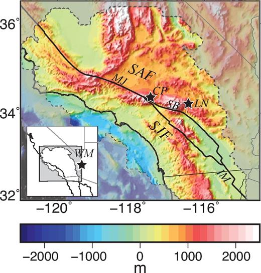
Southern California topography (Becker et al.2009), with major faults indicated as black lines (SAF, San Andreas Fault; SJF, San Jacinto Fault; IM, Imperial fault segment; MJ, Mojave segment). Dashed line and mask indicate regional focus of subsequent analyses (extent of observations from focal mechanisms, see Fig. 2a). Stars indicate locations of stress estimates from other studies discussed in the text (LN, Landers; CP, Cajon Pass; WM, Whipple Mountains).

Open in new tabDownload slide

There are four main assumptions that are made in the subsequent analysis. First, we assume that the stress tensor derived from earthquake focal mechanisms is representative of the orientation of the in situ stress field. Second, we assume that topography has been built to a critical state representing the transition between elastic behaviour and plastic failure. Third, we assume that topography, despite being on the verge of critical failure, is not the dominant component of the total stress field in southern California. Finally, we assume that the non-topographic sources of stress (mainly tectonic in origin) are dominant in southern California, to the extent that the orientation of the non-topographic stress field aligns with the orientation of the in situ stress field. In the sections below, we develop each of these assumptions in turn, and use them to derive lower bound estimates of stress magnitude in southern California. We then compare these estimates with independent estimates and observations of stress magnitude from complimentary methods.

2 METHODS

2.1 Total stress orientation

The modern 3-D in situ stress field within the seismogenic crust, σ, is the sum of the accumulated stress from multiple processes acting over multiple time scales, such as the tectonic driving stress field applied to the lithosphere over geologic time, the load of topography gradually built by brittle and ductile processes over millions of years, and the accumulation of stress due to shallowly locked fault segments throughout the earthquake cycle. While a long term goal of the geophysical community is to describe σ completely, direct observations of in situ stress are rare, owing to the difficulty of making such measurements (Zoback et al.2010). Those observations that are available primarily come from drilling for scientific or industrial purposes, where a combination of borehole breakouts and hydraulic fracturing can in some cases be used to estimate the full in situ stress tensor (e.g. Zoback & Healy 1992; Brudy et al.1997; Wilde & Stock 1997; Zajac & Stock 1997; Hickman & Zoback 2004). However, such observations are limited to locations where boreholes are present and where data have been made publically available. Also, these tend to be shallow crustal observations, within a kilometre or two from the surface, so it is not clear how well these observations represent the stress tensor at seismogenic depth (up to ∼10 km).

The deviatoric component of the in situ stress field, σ΄, is sometimes more easily identified, particularly the normalized deviatoric component, |${\boldsymbol{\sigma}}^{\prime}_{0}$|⁠, which describes the full 3-D tensor orientation of a stress field but lacks any information about stress magnitude (see Appendix A for a description of stress tensor metrics used in this study). One such source of orientation comes from indications of fault slip orientation, particularly when faults with a variety of different orientations and slip directions exist within a particular area (Angelier 1979; Angelier 1984; Michael 1984, 1987). While this method is applicable for any indication of slip rake, the most widely available slip indicators come from earthquake focal mechanisms. Yang et al. (2012) examined seismicity data from 1981–2010 in southern California and inverted these to yield a catalogue of 480 000 earthquakes, including focal mechanisms. Of these, 179 000 are considered highly reliable, based on the highest quality data. Yang & Hauksson (2013) then used the methods of Hardebeck & Michael (2006) to invert this focal mechanism catalogue for the 3-D deviatoric stress tensor orientation spanning a 5–10 km spaced grid across southern California. All recorded earthquakes contributed to the inversion, regardless of their hypocentre depth, so the resulting field represents the normalized (orientation only) stress state averaged over the seismogenic zone, with an interquartile depth range of 5–10 km (Hauksson et al.2012). Yang & Hauksson (2013) report an uncertainty in maximum principal stress azimuth of ±11° across most of the modelled region, though in some areas the uncertainty may be as high as ±30°. When comparing the results of this inversion to other stress fields, we therefore conservatively adopt a 3-D orientation misfit comparable to a difference of ±15° in the maximum horizontal principal stress azimuth (see Appendix A).

Fig. 2(a) shows the orientation of |${\bf Q}^{\prime}_{0}$|⁠, represented by the Anderson fault parameter A_ϕQ (see Appendix A for definitions of stress orientation metrics). As expected, much of southern California, particularly along the SAF and SJF segments, is observed to be in a strike-slip faulting regime, though some near fault areas are consistent with a thrust or normal regime, particularly along the Mojave and Imperial segments. Yang & Hauksson (2013) also describe the considerable heterogeneity in azimuth of the maximum horizontal principal stress, ranging within ±45°EofN across the modelled region and within ±30°EofN in the near-fault areas. Frictional theory predicts higher differential stresses in thrust regimes than in strike-slip or normal regimes when all other factors are equal (e.g. Zoback & Townend 2001), but observations of |${\bf Q}^{\prime}_{0}$| cannot be used on their own as a proxy for differential stress magnitude. Though this model provides a more complete characterization of the stress field orientation than has been available previously, a source of information separate from earthquake focal mechanisms is required to determine the stress field magnitude.

Figure 2.

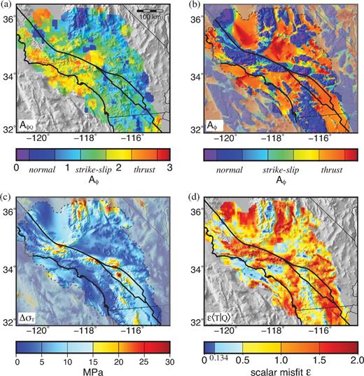
(a) Orientation of the in situ stress field derived from focal mechanisms (⁠|${\bf Q}^{\prime}_{0}$|⁠) as indicated by the Anderson fault parameter (A_ϕQ; Yang & Hauksson 2013). (b) Orientation (A_ϕT) and (c) differential stress magnitude (Δσ_T) of modelled crustal stress from topography at 5 km depth (approximate mean depth of the seismogenic zone). Masked region and faults as in Fig. 1. (d) Scalar 3-D misfit (ε) between normalized in situ stress field (⁠|${\bf Q}^{\prime}_{0}$|⁠) and crustal stress field from topography (T), with 0 indicating perfect alignment, 1 indicating arbitrary misalignment and 2 indicating perfect misalignment (Appendix A). Scalar misfit of ε = 0.134 corresponds to a difference in maximum horizontal principal stress azimuth of ±15°.

Open in new tabDownload slide

2.2 Stress field induced by topography

The orientation and magnitude of the crustal stress field due to topography are shown in Figs 2(b) and (c), respectively, at a depth of 5 km in the shallow seismogenic zone. As expected, the orientation of T, represented by the Anderson fault parameter A_ϕT (Fig. 2b) varies widely, with normal and thrust faulting regimes dominating in areas of high and low topography, respectively. The predicted differential stress due to topography (Δσ_T) (Fig. 2c) has peak magnitudes of ∼30 MPa, corresponding to the most rugged topography along the San Bernardino and Carrizo segments of the SAF, and along the southern Sierra Nevada mountains at the northern edge of the modelled region, while magnitudes of 10–20 MPa are common along the main segments of the SAF and SJF. It should be noted that the areas of lowest topography-induced stress are not the regions of lowest elevation (e.g. within the Salton Trough), but rather those with the lowest topographic gradient, such as the sedimentary basins along the coast or within the San Joaquin Valley.

2.3 Estimating total stress magnitude

This is equivalent to assuming that the orientation of in situ stress is unaffected by stress contributions from topography across southern California. In the most conservative case of a normal-oriented topographic stress field (A_ϕT = 0) and a strike-slip-oriented ‘other’ stress field (A_ϕX = 1.5), this assumption would hold as long as |${{\Delta {\sigma _T}} \mathord{/ {\vphantom {{\Delta {\sigma _T}} {\Delta {\sigma _X}}}} } {\Delta {\sigma _X}}} < 0.5$|⁠. In a more general case where either component exhibits obliquity, the magnitude of topographic stress can be even closer to that of the other stresses and still have this assumption hold.

The first assumption, that topography is not dominant, can be demonstrated by comparing the orientations of the topographic stress (T) with orientation of the in situ stress field (represented by |${\bf Q}^{\prime}_{0}$|⁠). Stress field orientations across the study region are compared using the scalar misfit operator ε, which describes the scalar misfit between two 3-D stress fields of arbitrarily different orientation based on their tensor dot product (eq. A3). Use of the ε operator allows us to compare the full 3-D orientations of these stress tensors with a single scalar value (ε ∈ [0, 2], with 0 indicating perfect alignment, 1 indicating arbitrary misalignment, and 2 indicating perfect misalignment). The misfit |$\varepsilon \langle {\bf Q}^{\prime}_0 \mathrel{ | {\vphantom {{{\bf Q}^{\prime}_0} {{\bf T}}}} } {{{\bf T}}} \rangle $| between T and |${\bf Q}^{\prime}_{0}$| across the region is shown in Fig. 2(d). Based on the uncertainties reported for the focal mechanism inversion by Yang & Hauksson (2013), we expect a perfectly aligned stress field to exhibit a scalar misfit of ε < 0.134, equivalent to a difference in maximum horizontal principal stress azimuth of ±15° (Fig. A1). However, only 2.5 per cent of the modelled region and 1.5 per cent of the near-fault area (<20 km from main SAF and SJF trace) fits to within this acceptable misfit tolerance. Furthermore, across 80 per cent of the modelled region and 86 per cent of the near-fault area, the scalar misfit parameter between these two stress fields exceeds 0.5 (equivalent to a difference in maximum horizontal principal stress azimuth of ±30°). That the orientations of T and |${\bf Q}^{\prime}_{0}$| differ so greatly is an indication that topography is not the dominant contribution to the stress field σ.

The second assumption, that the other sources of stress (mainly tectonic) that make up the X field are dominant, can similarly be demonstrated by comparing the orientations of X and |${\bf Q}^{\prime}_{0}$|⁠. Many researchers have used observations from GPS and InSAR to resolve tectonic strains across the region (e.g. Smith & Sandwell 2003; McCaffrey 2005; Meade & Hager 2005; Bird 2009; Smith-Konter & Sandwell 2009; Zeng & Shen 2010), and while the particular methods and the scope of questions asked by each study differ, the models agree remarkably well about the overall orientation of the strain field, especially in the highest strain rate areas along the SAF and SJF (Hearn et al.2010). We take these modelled strain rates to be a reasonable approximation of the orientation of the tectonic stress field |${\bf X}^{\prime}_0$|⁠. Previous comparisons between the azimuth of the maximum horizontal principal stress (Yang & Hauksson 2013) and the geodetically determined azimuth of maximum crustal shortening (Hearn et al.2010) reveal a mean deviation between the two of ∼5° across the modelled region, with a typical standard deviation of ∼15° (Hauksson & Sandwell 2013). That the alignment between these two fields differs by less than the uncertainty in the orientation of the |${\bf Q}^{\prime}_{0}$| field suggests it is reasonable to assume that these tectonic sources of stress are dominant across the study region.

3 RESULTS

Figure 3.

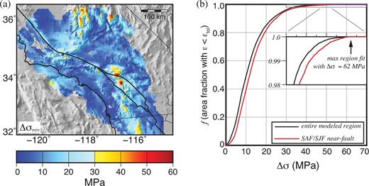
(a) Estimate of minimum differential stress (Δσ_min) satisfying eq. (6) across modelled region. Masked region and faults as in Fig. 1. (b) f, fraction of model region fit to better than ε < 0.134, for a given estimate of in situ differential stress magnitude. Black and red indicate full model region and near-fault regions (<20 km from main SAF or SJF trace) respectively. Inset figure is zoom of f > 0.98 region.

Open in new tabDownload slide

Because we have allowed for a considerable amount of uncertainty in the |${\bf Q}^{\prime}_{0}$| model, it is reasonable to expect that Δσ should satisfy eq. (5) across the entire modelled region. Accordingly, Fig. 3(b) shows the fraction f of both the entire modelled region and the near-fault area (<20 km from the main SAF and SJF trace) in which eq. (5) is satisfied as a function of Δσ. We find that most regions with low to moderate topography can be fit with relatively low stresses. For example, 85 per cent of the modelled region would be able to maintain the observed orientation |${\bf Q}^{\prime}_{0}$| with a minimum in situ differential stress magnitude of 20 MPa at seismogenic depth. However, the highest peaks in the San Bernardino and San Jacinto mountains require in excess of 62 MPa differential stress at seismogenic depth to support the observed topography, even when allowing for a conservative margin of misfit.

It is certainly possible that the magnitude of the stress field is laterally heterogeneous across the study region, particularly as the crustal basement terrain across southern California is heterogeneous. However, the pattern of required differential stress magnitude observed here does not seem to be correlated with crustal block strength (e.g. Matti et al.1992). A detailed investigation of the heterogeneity of stress magnitude in this region is beyond the scope of this study, but two end member cases can be assessed. If the variations in total stress magnitude are large compared to its mean, then the spatially varying Δσ_min in Fig. 3(a) would be appropriate to adopt as a minimum estimate. If, on the other hand, the variations in stress magnitude are small compared to its mean, such that total stress magnitude is approximately homogeneous, then that magnitude must be large enough to support even the most rugged topography. In this case, the best first order estimate of Δσ across the region would be the maximum observed 62 MPa. We consider both possibilities in the discussion that follows.

4 DISCUSSION

Though direct observations of in situ stress are rare, estimates of the magnitude of stress release throughout the earthquake cycle, in particular the coseismic stress drop, are more common. Observations of earthquake stress drop vary widely (∼0.05–30 MPa) but generally have a median value of ∼4–10 MPa (e.g. Brace & Byerlee 1966; Beeler et al.2001; Hardebeck & Hauksson 2001; Kanamori & Brodsky 2004; Allmann & Shearer 2007, 2009; Hauksson 2014). The stress drop, however, can only be related to the in situ stress field if additional assumptions are made, such as assuming complete stress release. Following the shallow 1992 M7.3 Landers earthquake, the in situ stress field was observed to rotate with post-seismic relaxation. This allowed Hardebeck & Hauksson (2001) to constrain the ratio of stress drop to deviatoric stress magnitude (measured as |${{( {{\sigma _1} - {\sigma _3}} )} \mathord{/ {\vphantom {{( {{\sigma _1} - {\sigma _3}} )} 2}} } 2}$|⁠) to be ∼0.6 (range of 0.25–1.0). Based on their estimate of stress drop on the various subsegments of the Landers rupture, these ratios correspond to a deviatoric stress magnitude of ∼10 MPa (range of 3.8–32 MPa). This corresponds to a differential stress magnitude (measured in this study as σ₁ − σ₃) of ∼20 MPa (range of 7.2–64 MPa) over the length scale of the rupture. This is consistent with the ∼20–30 MPa minimum in situ differential stress estimated for the Landers area in this study (Fig. 3a), but the upper range is also consistent with the homogeneous Δσ estimate over the entire region of 62 MPa. These observations are thus unable to discriminate between the homogeneous and heterogeneous Δσ estimates described above, and further observation will be required to constrain the degree of lateral heterogeneity in in situ stress magnitude.

Figure 4.

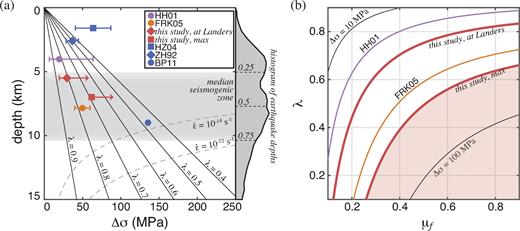
(a) Brittle yield strength in the upper crust for coefficient of friction μ_f = 0.6, with varying ratios of pore pressure to lithostatic pressure (λ) as indicated. Dashed grey lines represent ductile yield strength for given strain rate (e.g. Hirth et al.2001). Symbols indicate estimates of differential stress from previous studies: HH01 (Hardebeck & Hauksson 2001); FRK05 (Fialko et al.2005); HZ04 (Hickman & Zoback 2004); ZH92 (Zoback & Healy 1992); BP11 (Behr & Platt 2011). Minimum differential stress estimates from this study, both for the Landers area and the maximum across the study region, are indicated by red symbols, with upper bound arrows indicating that only the lower bound is constrained. Estimates from HH01, FRK05 and this study represent seismogenic depths. Histogram at right indicates depths of earthquakes used in focal mechanism inversion study (Hauksson et al.2012), with quartile depths indicated. (b) Contours of brittle yield strength at 5 km depth as a function of λ and μ_f. Red lines indicate μ_f and λ values consistent with the results of this study; shaded region shows the range of values permitted in this regional study. Purple and orange lines are based on differential stress estimates from HH01 and FRK05, respectively.

Open in new tabDownload slide

Fig. 4 also includes differential stress estimates from separate studies. Scientific drilling in Cajon Pass observed 37 ± 8 MPa differential stress at 2.6 km depth (Zoback & Healy 1992), while measurements made in the SAFOD borehole at Parkfield indicate 64 ± 23 MPa at 1.6 km depth (Hickman & Zoback 2004). Fialko et al. (2005) related variations in the orientation of the main SAF fault plane through the transverse ranges to the mean excess topography of the region, and concluded the upper crust must support an average differential stress of 40–60 MPa. This is slightly lower than the maximum estimate of this study, based on the most rugged topography, but this is expected as their estimate is based on a mean topography of ∼1.5 km, and does not consider topographic variations. Petrologic analysis, including paleopiezometry and thermobarometry, on exhumed crustal rocks from the Whipple Mountains in southern California has estimated mid-crustal differential stress peaks at 136 MPa at the brittle ductile transition (at a depth of ∼9 km) (Behr & Platt 2011), but then decreases to 13–17 MPa in the lower crust as ductile processes become more dominant (Behr & Hirth 2014). However, as these samples necessarily represent an earlier period of extension in this region, it is not clear how relevant these estimates are to present day crustal stress conditions. Nevertheless, the homogeneous end member estimate of differential stress presented in this study is generally consistent with estimates from these complimentary methods and with moderate values of coefficient of friction and pore pressure ratio (Fig. 4a). Only very low values of coefficient of static friction (μ_f < 0.3) or very high levels of pore pressure ratio (λ > 0.7) are prohibited by this analysis (Fig. 4b).

There is some evidence from laboratory studies that the b value of an earthquake catalogue is correlated to differential stress (e.g. Amitrano 2003), and some evidence from natural catalogues that b value decreases with depth (e.g. Mori & Abercrombie 1997; Spada et al.2013). This has led some to pose that earthquake catalogue b value be used to estimate stress values (Scholz 2015). This argument, however, is principally a restatement of the theoretical increase in differential stress with depth expected from brittle failure theory (e.g. Zoback & Townend 2001). Furthermore, Kamer & Hiemer (2015) estimated b values in the ANSS catalogue (1984–2014) to be uniform throughout southern California, with the possible exceptions of spatial variations attributable to aftershocks of the Northridge earthquake in the catalogue. We could, perhaps, take this as evidence of homogeneous stress, but it is more likely that b value estimations do not currently have the spatial resolution to conduct such an analysis. Overall, we find there are no stress estimates from b values in southern California that can be reliably included in this analysis.

As our estimate of differential stress magnitude does not include any a priori information about active faulting, it is instructive to consider the implications of our estimate for fault strength. It has long been recognized that the absence of a high heat flow anomaly along the SAF suggests that the SAF should sustain shear stress of no more than 20 MPa (e.g. Brune et al.1969; Lachenbruch & Sass 1980). Similarly, the relative angle between principal stress azimuth and fault strike (e.g. Zoback et al.1987; Hardebeck & Michael 2004; Townend & Zoback 2004), laboratory-based studies on fault gouge material (e.g. Lockner et al.2011), and numerical simulations of seismicity at depth (Bird & Kong 1994) suggest fault segments throughout the SAF system may be weak. A differential stress of ∼60 MPa in these regions would correspond to a maximum shear stress of 30 MPa, though shear stress could be lower in the event of non-optimal fault orientation. Overall, our estimate of in situ stress magnitude is consistent with previous observations that the SAF system is comprised of weak faults within an otherwise strong crust.

The conclusions of this study depend heavily on the assumption that the inverted stress field from earthquake focal mechanisms (Yang & Hauksson 2013) is a good estimate of the in situ stress field (eq. 1). However, not all areas across southern California are equally productive of seismicity. In particular, much of the seismicity near the SAF is not on the main San Andreas fault trace (Yang et al.2012), and it is possible that the absence of this seismicity biases the focal mechanism-based stress state inversion to be ‘less strike-slip’ than it actually is. In our results, however, we find that most of the main non-strike-slip areas along the SAF (Imperial Valley, along the Coachella segment, near the SAF-SJF intersection, and along the Mojave segment) are poorly fit to the topography model alone (Fig. 2), indicating that these regions are not artificially biasing the in situ magnitude estimate in those areas to be too low. On the other hand, as the topography model alone does not contribute strike-slip stresses in these regions, the possible underestimate of the strike-slip tendency of the stress field would not artificially bias the in situ magnitude estimate to be too high. In other words, the non-strike-slip regions of the SAF are not especially well-fit by the present analysis, nor would they become especially well-fit if these regions were enforced to be strike-slip. The overall effect on the results of this study would therefore be minimal. Only in the normal-oriented region in the north of the model space near Parkfield might the paucity of on-fault strike-slip earthquakes influence the differential stress magnitude estimate presented in Fig. 3(a).

Likewise, in this study, the value set for the acceptable misfit ε_tol is key for establishing the minimum estimate of in situ stress. The value of ε_tol should represent the larger of either (i) the extent to which |${\bf Q}^{\prime}_{0}$| is unknown (i.e. the uncertainty in the focal mechanism inversion); or (ii) the extent to which error is introduced by the simplifications of eq. (2) (i.e. by neglecting factors not explicitly accounted for here, such as localized fault processes, crustal heterogeneity, or depth dependent in situ stress); or (iii) the extent to which the assumption that tectonic driving stress is dominant (eq. 3) is flawed (i.e. the maximum influence that the neglected topography component is allowed to have). Because the observed misalignment between the tectonic and in situ stress fields (Hauksson & Sandwell 2013) is smaller than the reported uncertainty in the focal mechanism inversion (Yang & Hauksson 2013), it is appropriate to conservatively adopt the latter as our 3-D orientation misfit tolerance value. Were we to adopt a larger value for ε_tol (e.g. ε_tol = 0.5), the minimum required in situ stress magnitude estimate (Fig. 3a) would be lower. Such a larger tolerance may be appropriate in subregions where the principal assumptions of this study break down, such as in the southern Sierra Nevada where topography may be in a state of collapse and not fully supported.

5 CONCLUSIONS

In summary, we have developed an estimate of the in situ differential stress magnitude by adopting the in situ orientation indicated by earthquake focal mechanisms, and identifying the minimum differential stress magnitude required to support the load of topography. In doing so, we have presented a new estimate for crustal stress variations induced by surface and Moho topography in southern California based on methods previously applied to other plate boundary systems. We find that while regions with little topographic variation could be supported by a differential stress of ∼20 MPa, the most rugged regions across southern California, and along the SAF and SJF in particular, require in situ differential stress to have a magnitude of at least 62 MPa at seismogenic depth in order to sustain the in situ orientation indicated by focal mechanisms. If the magnitude of the in situ stress field is approximately homogeneous, this serves as a first order estimate of that magnitude across southern California. This result is supported by direct estimates of in situ stress derived from earthquake stress drops, borehole observations, and petrologic studies, and is consistent with theoretical estimates of brittle failure stress for moderate levels of friction (μ_f > 0.3) and pore pressure (λ < 0.7).

Acknowledgements

We are grateful to David Sandwell, Jeanne Hardebeck, Debi Kilb, Michelle Cooke and the members of the SCEC Community Stress Model working group for their valuable discussions, and to the anonymous reviewers and editor for helpful suggestions that improved the manuscript. This research was supported by the NSF award EAR-1439697 and the Southern California Earthquake Center (Contribution No. 6064). SCEC is funded by NSF Cooperative Agreement EAR-1033462 & USGS Cooperative Agreement G12AC20038.

REFERENCES

APPENDIX A: TREATMENT OF STRESS FIELDS

A stress field is a tensor field with six independent components that each vary in space and time. It can be difficult to conceptualize or visualize a fully 3-D stress field, so it is helpful to consider the orientation and magnitude of the stress field separately.

In general, the magnitude of a stress tensor is indicated by the three principal stresses, σ₁, σ₂, and σ₃. It is useful to define a scalar magnitude parameter that is some combination of these stresses, and in this study we will refer to the differential stress Δσ = σ₁ − σ₃. This metric has the advantage of simplicity, and gives comparable results to other more intricate metrics, such as the second invariant of the deviatoric stress field.

The scalar misfit ε ∈ [0, 2] is defined such that ε = 0 indicates A and B are in perfect alignment (i.e. all three principal axes are perfectly aligned), ε = 2 indicates A and B are in perfect misalignment (i.e. principal axes are aligned, but mis-ordered), and ε = 1 indicates A and B are arbitrarily misaligned.

Though scalar misfit ε incorporates 3-D differences between stress tensors, it is helpful for interpretation to consider how horizontal stress rotation, that is, a difference in azimuth only (Δθ), would be manifest in the ε value. Fig. A1 demonstrates this nonlinear relationship, where for example, ε values of 0.05, 0.134, and 0.25 correspond to Δθ values of ±8°, ±15°, and ±22° respectively.

Figure A1.

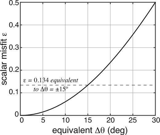
Scalar misfit ε for two arbitrary stress fields whose orientations differ only in azimuth (i.e. equal A_ϕ values, but different θ values). Dashed line indicates ε value corresponding to Δθ = ±15°.

Open in new tabDownload slide

Because stress fields in general vary spatially, scalar misfit ε will also vary spatially as a point-by-point comparison of A and B. In order to quantify the overall fit of a broad regional model, we could take the mean or median of the misfit over a region. However, we are generally more interested in finding a model stress tensor that fits the broad region reasonably well than we are in fitting a few locations extremely well. For this reason, we define a misfit tolerance based on observational uncertainty of ε_tol = 0.134 (comparable to Δθ = ±15°), and define f ∈ [0, 1] to be the fraction of a given region or subregion with ε < ε_tol (e.g. f = 0.9 indicates that at 90 per cent of the model points within a considered region, the two stress tensors have the same orientation to within tolerance).

APPENDIX B: CRUSTAL STRESS FROM LOAD OF TOPOGRAPHY

Topography gradually develops through a complex set of processes involving driving forces, elastic bending and compression, permanent deformation via brittle and ductile failure, isostatic rebound, and erosion all working to both build and collapse topography over time. Modelling each of these processes deterministically is untenable due to our incomplete knowledge of a region's geologic history. However, it has been observed that such systems tend to reach a critical state in which the forces creating the topography are in equilibrium with the forces relaxing the topography (e.g. Dahlen 1990). This is equivalent to assuming the crust has an elastic-perfectly-plastic rheology, in which material behaves elastically up to some critical yield stress threshold, but any additional stress beyond that threshold results in permanent plastic deformation (Fig. B1a). If this is the case, then the elevation and ruggedness of the topography itself is an indicator of the stress being supported within the crust.

Figure B1.

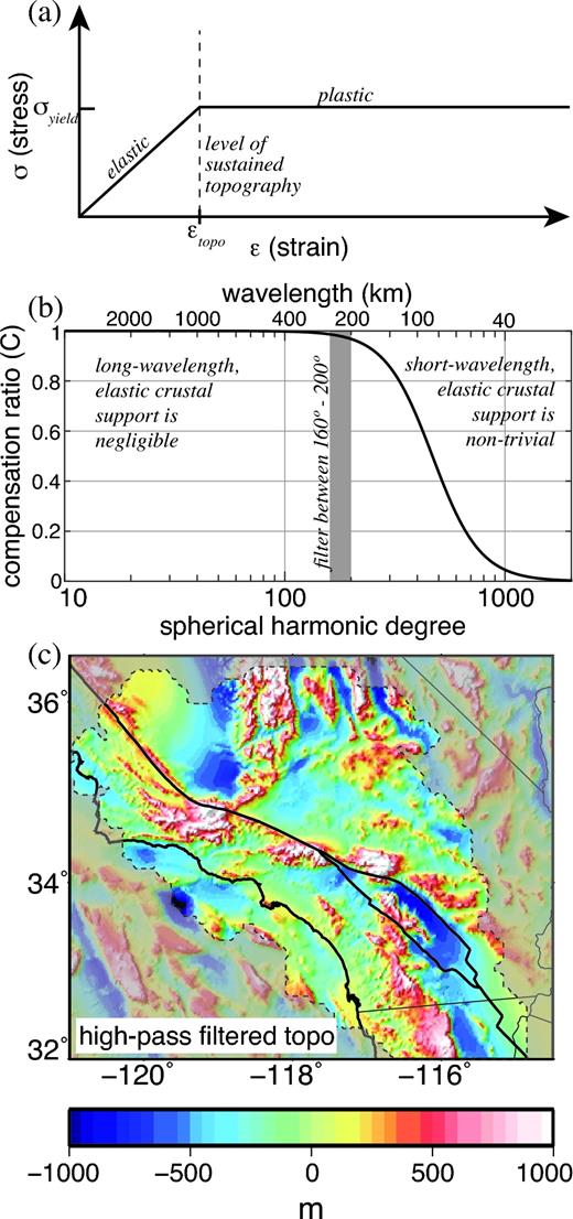
(a) Generalized elastic-perfectly-plastic rheology in which level of sustained topography ε_topo is indicative of critical yield stress threshold σ_yield. (b) Compensation ratio C of isostatic support to elastic support, as a function of spherical harmonic degree (wavelength). (c) Short-wavelength topography supported by stress variations within the crust, high-pass filtered between spherical harmonic degree 160°–200° (∼200–250 km), grey band in (b). Fault lines and shaded regions as in Fig. 1.

Open in new tabDownload slide

We can take advantage of this observation by assuming that the current topography in southern California represents the critical elastic endmember of built topography, right on the verge of plastic failure in the crust. This stress state is calculated by loading an elastic crust from above with the load of current surface topography (Becker et al.2009) and from below with the buoyant load of Moho topography. However, not all wavelengths of topography are supported by stresses within the crust. The longest wavelength features (e.g. the transition from continent to ocean or the rise of major mountain ranges such as the Sierra Nevada) are principally supported by isostasy in the mantle, and therefore do not contribute to crustal stress variations beyond the increase in lithostatic stress. More localized topographic features, on the other hand, are supported within the crust through a combination of isostasy and internal deformation.

We filter the topography load with a cosine-squared taper between spherical harmonic degree 160–200 (wavelengths 200–250 km, ∼2πh), which correspond to a compensation ratio of C = 0.97–0.99. The resulting high-pass topography (Fig. B1c) includes all wavelengths for which elastic support is non-trivial, while omitting wavelengths that are almost entirely supported by the mantle. Accordingly, this short wavelength filtered topography maintains the ruggedness of peaks throughout southern California, particularly along the SAF, but removes the longest wavelength signal of the transition between oceanic and continental crust and the continental rifting of the Salton Trough (compare with Fig. 1).

The shape of the buoyant load applied at the Moho is assumed to be related to the applied surface topography load via flexure, such that the crust supports some small but finite internal elastic bending (Watts 2001). The effective elastic thickness of the crust, T_e, is assessed by comparing the observed gravity anomaly (Sandwell et al.2014) with a suite of gravity models representing the different Moho shapes predicted for different values of T_e (Fig. B2 ; Watts 2001; Luttrell & Sandwell 2012). We calculate the gravity anomaly from the short-wavelength filtered topography using the first term of the gravity expansion of Parker (1972) for a homogeneous single-layer crust of density 2800 kg m⁻³ and thickness 35 km overlying a homogeneous mantle of density 3300 kg m⁻³, assuming a Young's modulus of 70 GPa and a Poisson's ratio of 0.5, corresponding to an incompressible elastic solid. We compare these to the observed gravity, filtered over the same wavelengths as topography (Fig. B2a), focusing on regions that are included in the focal mechanism model |${\bf Q}^{\prime}_{0}$| (Fig. 2; Yang & Hauksson 2013). Fig. B2(b) shows the variation in model RMS across the model region as a function of T_e, with a best fitting effective elastic thickness of 3 km. This T_e result is robust to the choice of filtering wavelength of the topography load.

Figure B2.

(a) Observed gravity anomaly (Sandwell et al.2014), with fault lines and shaded regions as in Fig. 1. (b) Gravity model RMS as a function of elastic thickness. Best fit to observations is achieved with elastic thickness T_e = 3 km.

Open in new tabDownload slide

With the appropriate loads at the surface and Moho defined, we calculate the stress field induced in an elastic crust, representing the critical transition from elastic to plastic failure. The method used here was first developed by Luttrell et al. (2011) to assess stress state in the vicinity of the 2010 Maule, Chile earthquake and later adopted by Luttrell & Sandwell (2012) to constrain tectonic driving stresses acting along the global mid-ocean ridge. The model performs a semi-analytic (pseudospectral) calculation using a Green's function for a point normal traction on the surface of a thick elastic plate and a non-identical buoyant point normal traction at the base of the plate, representing the buoyant load applied by the Moho (for a complete derivation of this solution, see appendix A of Luttrell et al.2011). This Green's function is then convolved with the spatially varying surface load from topography, applied as a normal traction at elevation 0 km, and the spatially varying buoyant Moho load, applied as a normal traction at the base of the crust (in this case, elevation −35 km). The resulting calculation is fully depth dependent and 3-dimensional within the crust. Note that because we are concerned with seismogenic depths (interquartile range 5–10 km), we neglect surface shear tractions exerted by rugged topography, which mainly influence the top ∼1 km of the crust (approximately half the height of the topography) (Liu & Zoback 1992). Convolution is performed in the Fourier domain, so that the calculation is numerically efficient, regardless of the complexity of the load surfaces. The resulting 3-D field serves as T, our estimate of the crustal stress field from the load of topography.