


Abstract
We study rapidly rotating Boussinesq convection driven by internal heating in a full sphere. We use a numerical model based on the quasi-geostrophic approximation for the velocity field, whereas the temperature field is 3-D. This approximation allows us to perform simulations for Ekman numbers down to 10−8, Prandtl numbers relevant for liquid metals (∼10−1) and Reynolds numbers up to 3 × 10⁴. Persistent zonal flows composed of multiple jets form as a result of the mixing of potential vorticity. For the largest Rayleigh numbers computed, the zonal velocity is larger than the convective velocity despite the presence of boundary friction. The convective structures and the zonal jets widen when the thermal forcing increases. Prograde and retrograde zonal jets are dynamically different: in the prograde jets (which correspond to weak potential vorticity gradients) the convection transports heat efficiently and the mean temperature tends to be homogenized; by contrast, in the cores of the retrograde jets (which correspond to steep gradients of potential vorticity) the dynamics is dominated by the propagation of Rossby waves, resulting in the formation of steep mean temperature gradients and the dominance of conduction in the heat transfer process. Consequently, in quasi-geostrophic systems, the width of the retrograde zonal jets controls the efficiency of the heat transfer.
1 INTRODUCTION
Convection is the main heat transport process in the liquid cores of planets and is thought to be responsible for the generation of planetary magnetic fields. Convection is strongly affected by the rapid rotation of the planet via the action of the Coriolis force. Owing to the very low fluid viscosity, the convective flows are turbulent, although the nonlinear inertial effects are relatively weak compared with the Coriolis force. Under these conditions, and in the absence of magnetic fields, the primary dynamical balance is established between the Coriolis force and the pressure gradient and is called geostrophic balance. Geostrophic flows are invariant along the rotation axis, and so, in spherical geometry, they can only be axisymmetric and azimuthal (i.e. zonal). Convective flows, which are directed along the direction of gravity, cannot be exactly geostrophic, but nevertheless form tall columnar flows aligned with the rotation axis (Jones 2015); such flows are commonly referred to as ‘quasi-geostrophic’ (QG). These columnar convective flows produce coherent Reynolds stresses that drive geostrophic zonal flows (Gilman 1977; Busse & Hood 1982). Stress-free boundary conditions, where boundary friction is absent, favour the emergence of strong zonal flows (e.g. Aurnou & Olson 2001). In models with relatively small viscosity (which can be measured by the Ekman number, the ratio of the rotation period to the global viscous timescale), the zonal flows develop persistent multiple jets of alternating sign inside the tangent cylinder (e.g. Heimpel et al. 2005; Gastine et al. 2014). The observation of intense jets in geophysical and astrophysical objects (e.g. Schou et al. 1998; Porco et al. 2003; Livermore et al. 2017) has prompted much effort dedicated to their study, and in particular, their width and amplitude (e.g. Christensen 2002; Gillet et al. 2007; Read et al. 2015; Cabanes et al. 2017). Although zonal flows (and shear flows in general) do not transport heat outwards, they strongly affect the convection because they can deflect and shear the convective flows, thereby reducing the efficiency of the heat transfer (e.g. Aurnou et al. 2008; Goluskin et al. 2014; von Hardenberg et al. 2015; Yadav et al. 2016). In the present paper, we explore the effect of intense, multiple zonal jets on the convective heat transport in turbulent rotating convection for small Ekman numbers.
The numerical modelling of turbulent rotating flows is extremely challenging as it necessitates a wide range of dynamical length and time scales. Numerical models must therefore employ Ekman numbers that are several orders of magnitude larger than those found in natural objects. However, in the absence of magnetic fields, the lengthscale of the convective flows scales with the Ekman number, at least at the linear onset of convection. The coherence of the Reynolds stresses, and hence the width and amplitude of the zonal flows, might well be affected by the convective lengthscale, and thus by the Ekman number. In order to approach turbulent rotationally constrained convection at small Ekman numbers, we alleviate part of the computational limitations by using a QG approximation that was developed by Busse & Or (1986) for thermal convection in the annulus geometry of Busse (1970) with curved boundaries. The model neglects the variations of the axial vorticity of the flow along the rotation axis, which allows to compute the velocity in 2-D. This is an important limitation to the full dynamics of rotating convection (e.g. Calkins et al. 2013), but the rationale of using this QG model is that it allows the exploration of currently inaccessible regions of the parameter space, thereby informing future 3-D studies. Variations of the QG model have been successfully applied in numerous studies in spherical geometry (e.g. Cardin & Olson 1994; Morin & Dormy 2004; Calkins et al. 2012). Where possible, results from these studies have been successfully benchmarked against asymptotic theories (Gillet & Jones 2006; Labbé et al. 2015), 3-D numerical models (Aubert et al. 2003; Plaut et al. 2008), and laboratory experiments (Aubert et al. 2003; Schaeffer & Cardin 2005; Gillet et al. 2007).
Following the model constructed in Guervilly & Cardin (2016), we use a hybrid numerical model that couples the QG velocity to a 3-D implementation of the temperature in the whole sphere, in order to account for the spherical symmetry of the basic temperature background. The buoyancy driving is controlled by the temperature averaged along the direction of the rotation axis, which, contrary to QG models using a 2-D temperature field (Busse & Or 1986), is not assumed to be equal to the temperature in the equatorial plane. Solving the temperature in 3-D will allow us to assess the influence of the 3-D temperature on the QG dynamics. This implementation is particularly appropriate to model fluids with small Prandtl numbers (the ratio of the viscosity to the thermal diffusivity) that are typical of liquid metals (|$\mathcal {O}(10^{-1})$|) by permitting the use of a 3-D grid for the temperature that is coarser than the 2-D grid used for the velocity. For simplicity, we consider only thermal convection in a full sphere without a solid inner core. The thermal convection is driven by a homogenous internal heating, which is more relevant for the early history of the Earth's core.
The existence of a so-called strong branch of convection driven by internal heating, as first suggested by the weakly nonlinear analysis of Soward (1977), was recently found numerically by Guervilly & Cardin (2016) with the hybrid QG-3D model and by Kaplan et al. (2017) with a fully 3-D model for Ekman numbers smaller than |$\mathcal {O}(10^{-7})$| and Prandtl numbers smaller than unity. The bifurcation is subcritical at the onset of convection and the strong branch is characterized by Reynolds numbers greater than 1000 near the onset and strong zonal flows. In this paper, we focus on the production of zonal flows on this strong branch of convection for Ek ∈ [10−8, 10−7] and Pr ∈ [10−2, 10−1].
The layout of the paper is as follows. In Section 2, we detail the formulation of the hybrid QG-3D model. In Section 3, we describe the radial dependence of the convection and zonal flows and quantify the dependence of the jet width, convective lengthscale and zonal flow velocity on the model parameters. The drift and stability of the zonal flows is discussed in Section 4 and their mechanism of formation in Section 5. The effect of the zonal flows on the heat transport is presented in Section 6. Finally, a discussion of the results is given in Section 7.
2 MATHEMATICAL FORMULATION
Throughout this paper, we use both spherical coordinates (r, θ, ϕ) and cylindrical polar coordinates (s, ϕ, z). The mathematical formulation and the numerical method are described in detail in Guervilly & Cardin (2016), where the linearized version of the code is benchmarked against theoretical and previous numerical results at the onset of convection. The governing equations and the assumptions of the model are briefly described below.
2.1 Governing equation for the non-axisymmetric flow
To model the system of eqs (2)–(4) for small Ekman and Rossby numbers, we use the QG approximation to model the evolution of the velocity field (e.g. Or & Busse 1987; Cardin & Olson 1994; Gillet & Jones 2006). The QG approximation reduces the 3-D system to a 2-D system by taking advantage of the small variations of the flow along z compared with variations in s and ϕ due to the rapid rotation. This approximation is only justified in the case of small slope of the boundaries, such as the Busse (1970) annulus. In the case of a sphere, the approximation is therefore not rigorously justified in any asymptotic limit. Consequently, our QG model is intended as a simplified model of convection in a rapidly rotating sphere that allows us to investigate unexplored regions of the parameter space. When possible, comparisons with theoretical, experimental and 3-D numerical models show that the QG model correctly reproduces key properties of the full system (Aubert et al. 2003; Morin & Dormy 2004; Gillet & Jones 2006; Gillet et al. 2007; Plaut et al. 2008).
The numerical code solves the evolution equation of the non-axisymmetric streamfunction ψ. The no-slip and impenetrable boundary conditions imply that ψ = ∂sψ = 0 at s = 1. We use the regularity condition |$\hat{\psi }^m=\mathcal {O}(s^m)$| at s = 0, where |$\hat{\psi }^m(s,t)$| is the Fourier mode of azimuthal wavenumber m (see Guervilly & Cardin 2016, for more detail).
2.2 Governing equation for the zonal flow
2.3 Governing equation for the temperature
2.4 Numerical method
In the following, the superscripts g are removed for clarity. The evolution equations for ψ and |$\overline{u_{\phi }}$| are solved on a 2-D grid in the equatorial plane. A second-order finite difference scheme is implemented in radius with irregular spacing (finer near the outer boundary). In the azimuthal direction, the variables are expanded in Fourier modes. The evolution equation for the temperature is solved on a 3-D grid. Similarly to the 2-D grid, a finite difference scheme is used in radius. The temperature is expanded in spherical harmonics |$Y_l^m$| in the angular coordinates with l representing the latitudinal degree and m the azimuthal mode. Further detail about the numerical interpolations between the 2-D and 3-D grids used to compute the buoyancy term and the advection of the temperature can be found in Guervilly & Cardin (2016) and Guervilly (2010).
List of input and output parameters for all the simulations presented in the paper. Rec and Re0 are the convective and zonal Reynolds numbers, respectively. The columns labelled |$(N^u_s,M^u_{\rm max})$| and |$(N^t_r,M^t_{\rm max},L^t_{\rm max})$| give the numerical resolutions on the 2-D and 3-D grids, respectively. The last column gives the integration time used to compute the time averages in units of 1/Ω and, in brackets, in units of a convective turnover timescale, lc/Uc, where Uc is the r.m.s. convective velocity (equivalent to Rec in our dimensionless units) and lc is the convective lengthscale computed from eq. (23) and averaged between 0.1 ≤ s ≤ 0.8.
| Ek | Pr | Ra | Ra/Rac | Rec | Re0 | |$(N^u_s,M^u_{\rm max})$| | |$(N^t_r,M^t_{\rm max},L^t_{\rm max})$| | Integration time |
|---|---|---|---|---|---|---|---|---|
| 10−7 | 10−1 | 6 × 10⁹ | 1.19 | 1012 | 445 | (1100, 200) | (500, 150, 150) | 3 × 10⁵ (479) |
| 10−7 | 10−1 | 1 × 10¹⁰ | 1.99 | 2070 | 1110 | (1100, 200) | (500, 150, 150) | 3 × 10⁵ (794) |
| 10−7 | 10−1 | 2 × 10¹⁰ | 3.97 | 3663 | 2994 | (1200, 200) | (500, 150, 150) | 105 (414) |
| 10−7 | 10−1 | 3 × 10¹⁰ | 5.96 | 5093 | 5064 | (1200, 200) | (500, 150, 150) | 104 (54) |
| 10−7 | 10−1 | 4 × 10¹⁰ | 7.95 | 6243 | 6840 | (1200, 200) | (500, 150, 150) | 104 (61) |
| 10−7 | 10−1 | 5 × 10¹⁰ | 9.94 | 7731 | 9515 | (1500, 260) | (600, 180, 180) | 104 (73) |
| 10−7 | 10−2 | 1.9 × 10⁹ | 1.05 | 5215 | 5710 | (1000, 160) | (400, 96, 96) | 2 × 10⁴ (90) |
| 10−7 | 10−2 | 3 × 10⁹ | 1.65 | 9027 | 11708 | (1000, 160) | (400, 96, 96) | 104 (67) |
| 10−7 | 10−2 | 4.8 × 10⁹ | 2.64 | 11487 | 21834 | (1200, 180) | (400, 96, 96) | 104 (82) |
| 10−7 | 10−2 | 8.5 × 10⁹ | 4.68 | 17548 | 40009 | (1400, 200) | (400, 96, 96) | 104 (105) |
| 10−8 | 10−1 | 7.45 × 10¹⁰ | 0.96 | 855 | 243 | (1600, 256) | (700, 200, 200) | 2 × 10⁶ (633) |
| 10−8 | 10−1 | 7.8 × 10¹⁰ | 1.01 | 1047 | 291 | (1600, 256) | (700, 200, 200) | 2 × 10⁶ (785) |
| 10−8 | 10−1 | 1.5 × 10¹¹ | 1.93 | 3393 | 1128 | (1800, 280) | (700, 200, 200) | 5 × 10⁵ (400) |
| 10−8 | 10−1 | 2 × 10¹¹ | 2.58 | 4876 | 1893 | (1800, 280) | (700, 200, 200) | 5 × 10⁵ (506) |
| 10−8 | 10−1 | 3 × 10¹¹ | 3.87 | 7108 | 4724 | (1800, 280) | (700, 200, 200) | 2 × 10⁵ (286) |
| 10−8 | 10−1 | 5 × 10¹¹ | 6.44 | 9920 | 9341 | (1900, 300) | (700, 200, 200) | 105 (191) |
| 10−8 | 10−1 | 7 × 10¹¹ | 9.02 | 12023 | 13176 | (2000, 320) | (750, 200, 200) | 2 × 10⁶ (4453) |
| 10−8 | 10−2 | 2 × 10¹⁰ | 0.68 | 7200 | 4753 | (1400, 220) | (500, 128, 128) | 2 × 10⁵ (216) |
| 10−8 | 10−2 | 3 × 10¹⁰ | 1.01 | 13498 | 10598 | (1400, 220) | (500, 128, 128) | 105 (177) |
| 10−8 | 10−2 | 5 × 10¹⁰ | 1.69 | 23288 | 23309 | (1500, 240) | (500, 128, 128) | 4 × 10⁴ (108) |
| 10−8 | 10−2 | 8 × 10¹⁰ | 2.70 | 33163 | 43609 | (1600, 260) | (500, 128, 128) | 5 × 10⁴ (191) |
3 STRUCTURE OF THE CONVECTIVE AND ZONAL FLOWS AND SCALING OF THE VELOCITY
3.1 Radial dependence of the convection
In this section, the Ekman and Prandtl numbers are fixed to Ek = 10−8 and Pr = 10−1. For these parameters, the stable solution is located on a strong branch of convection, which is discontinuous at the onset of convection (Guervilly & Cardin 2016; Kaplan et al. 2017). All cases presented in this paper are located on the strong branch. This branch is distinct from the weak branch of convection, which occurs for |$\mbox{{Ek}}\mbox{{Pr}}\gtrsim \mathcal {O}(10^{-8})$| and is continuous at the onset of convection. At the onset of convection, solutions on the weak branch take the form of propagating structures that are tilted in the prograde direction. These structures are known as thermal Rossby waves and have been extensively studied in the literature (e.g. Busse 1970; Zhang 1992). Near the onset of convection, the flows on the strong branch are starkly different and are described in detail below.
For Ek = 10−8 and Pr = 10−1, the nonlinear convection is maintained below the linear onset of convection (quantified by the critical Rayleigh number Rac), down to a value Ra = 0.96Rac (Guervilly & Cardin 2016). We vary the Rayleigh number from this lower value to approximately 9Rac. Fig. 1 shows snapshots of the radial and azimuthal velocities in the equatorial plane for Ra/Rac = 0.96, Ra/Rac = 1.93 and Ra/Rac = 9.02. In all three cases, two dynamical regions can be distinguished: an inner region, where the convection is vigorous with values of the radial velocity up to 3000 for the lowest Ra and up to 30 000 for the largest Ra, and an outer region, where the radial flow has smaller amplitude and the flow has finer structures that are tilted in the prograde direction. This radial dependence of the convection, sometimes referred to as dual convection, was previously described in laboratory experiments (Sumita & Olson 2000) and QG (Aubert et al. 2003) and 3-D numerical models (Miyagoshi et al. 2010). The limit between the two regions is located around s = 0.5 for the lowest Ra and s = 0.8 for the largest Ra, so the limit moves outwards when the convection becomes more vigorous. In the inner region, the convective flows are strongly time dependent, especially for large Ra, and are subject to frequent nonlinear interactions. The contours of the radial velocity tend to be directed radially, contrary to the tilted contours of the outer region. For large Ra, the azimuthal lengthscales of the radial flow decreases with increasing radius. This is likely due to the increase of the slope of the boundary β with radius: the vortex stretching term in the axial vorticity equation, which depends on β, impedes the radial motion of wide vortices. The azimuthal extent of the convective flows clearly increases with Ra, which indicates the presence of an upscale energy transfer as expected in β-plane turbulence (e.g. Davidson 2013). For all Rayleigh numbers, the radial velocity is weak in the central region because the gravity goes to zero at the centre. In the outer region, β is large and the vortex stretching term is the dominant source of the axial vorticity, so this outer region is dominated by the propagation of Rossby waves. The nonlinear interactions are weaker in this region.
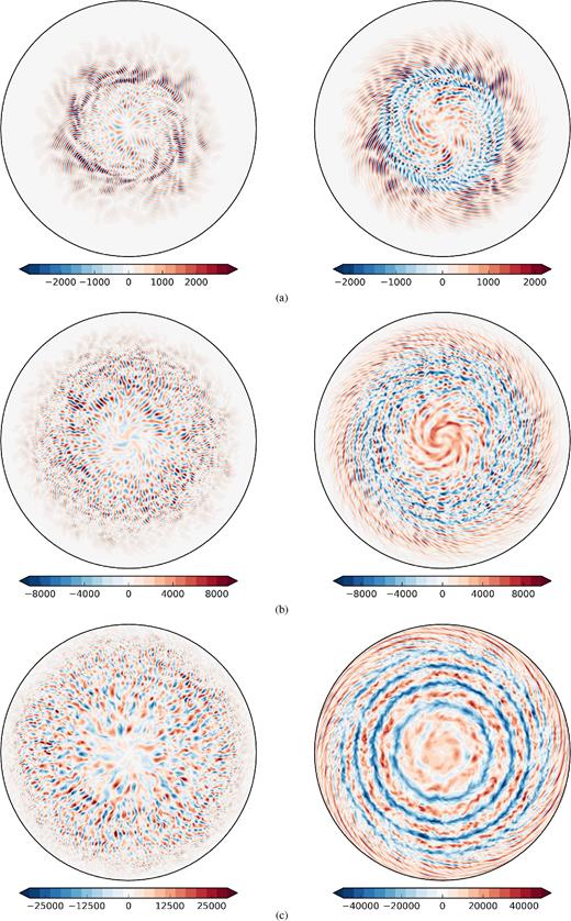
Snapshots of the radial velocity (left) and the azimuthal velocity (right) in the equatorial plane for Ek = 10−8 and Pr = 10−1 for (a) Ra/Rac = 0.96, (b) Ra/Rac = 1.93 and (c) Ra/Rac = 9.02.
For all Ra, the azimuthal flow has a visible axisymmetric (i.e. zonal) component. Fig. 2 shows the time-averaged profiles of the zonal flow for different Ra. The zonal flow is prograde in the outermost region for all Ra. In the outer region dominated by Rossby waves, the Reynolds stresses due to the correlation of the velocity along the tilted contours produce a prograde jet in the outer part and a neighbouring inner retrograde jet (e.g. Busse & Hood 1982). The behaviour of the zonal flow in the inner convective region is different depending on Ra. For the lowest Ra in Fig. 1, azimuthal flows appear to spiral inward from mid-radius. These flows have an axisymmetric average that is positive in the centre and negative near s = 0.4. The time-averaged profile of the zonal flow for this Ra has therefore three jets of alternating sign. For Ra/Rac = 1.93, the azimuthal flows consist in a multitude of meandering narrow jets. Around mid-radius, the azimuthal average of the narrow meandering jets is not well-defined. Their axisymmetric average is mostly negative because the retrograde jets have stronger amplitude. In the centre, the azimuthal flow has a clear prograde direction and is wider than the meandering jets at larger radius. For Ra/Rac = 9.02, the multiple azimuthal jets have stronger velocity than the radial flow and they do not meander so their net axisymmetric average is well-defined. The radial profile of the zonal flow shows persistent multiple jets. The central jet remains prograde and is wider than the jets located at larger radius. Overall, for Ra > 3Rac, the zonal flows develop persistent multiple jets and the innermost and outermost jets always remain prograde. The region occupied by the in-between jets becomes wider as Ra increases and the limit between inner convective region and outer Rossby wave region moves outwards. A thin viscous boundary layer can be observed on the profiles of the zonal flow of the largest Rayleigh number as the boundary condition is no-slip at s = 1. This thin boundary layer is well resolved in our model as the radial grid is refined near the boundary.
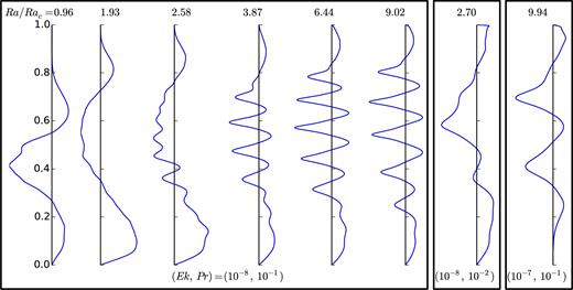
Radial profile of the zonal flow (time average) for different Rayleigh numbers (indicated at the top of each subplot) and Ekman and Prandtl numbers (indicated at the bottom). The vertical axis is the radius. The range of the horizontal axis is different for each subplot: the maximum of the zonal flow increases 80-fold between the smallest and largest Rayleigh numbers for Ek = 10−8 and Pr = 10−1.
For large Ra, the zonal velocity is larger than the radial velocity. In this case, the radial shear exerted by the zonal flow can be faster than the vortex turnover timescale, so the zonal flow has a dominant role in the dynamics of the convective vortices. The radial flow has a smaller radial extent at the larger Ra due to the presence of the multiple zonal jets of strong amplitude. The convective structures then change from narrow in ϕ and extended in r to fatter in ϕ and shortened in r as Ra increases.
3.2 Zonal jet width and convective lengthscale
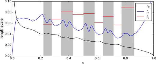
Radial profiles of the Rhines scale lR, the integral scale of the convective flow lc and the width of the jets lj for Ek = 10−8, Ra/Rac = 9.02 at Pr = 10−1. The grey bands correspond to the regions where the zonal flow is retrograde.
As the Rayleigh number (and thus U) increases, the Rhines scale predicts that the most energetic convective eddies become larger. This is indeed what we observe qualitatively on the snapshots of Fig. 1. This increase of the convective scale should be accompanied by an increase of the jet width. Fig. 2 shows that the jets indeed tend to become wider when the Rayleigh number increases. However this increase might be due to the widening of the inner convective region as it pushes the outer region outwards. Larger Ra, currently out of reach of our computational capabilities, would be necessary to observe a sizeable increase in the size of the jets.
We can extend our study on the zonal and convective lengthscales and the predictive value of the Rhines scale from the results of simulations performed at different Ek and Pr. We cannot presently run simulations at Ek < 10−8, so this study is restricted to higher Ek, namely Ek = 10−7. Our QG-3D model allows us to explore small Pr, so we also use results from calculations at Pr = 10−2. The two panels on the right of Fig. 2 shows the zonal velocity for (Ek, Pr) = (10−8, 10−2) and (Ek, Pr) = (10−7, 10−1) at the largest Ra performed (see Table 1). For (Ek, Pr) = (10−7, 10−1), the zonal flow has 5 jets of alternating sign. The zonal jets widen when the Ekman number increases if this leads to a larger r.m.s. convective velocity Ek U according to the Rhines scale (24).
For (Ek, Pr) = (10−8, 10−2), the time-averaged zonal flow also has five alternating jets. By visual inspection of the snapshots of the velocity, it appears that meandering azimuthal flows are present in the inner region, similarly to the case Ra = 1.93 for (Ek, Pr) = (10−8, 10−1). This suggests that larger Rayleigh numbers would be necessary to get multiple persistent jets. However, we were not able to perform calculations at larger Ra to confirm this. Smaller values of Pr lead to larger values of the convective velocity (see Table 1), and hence, to wider jets.
To compare more systematically the convective lengthscale with the Rhines scale, Fig. 4 shows the values of lc versus lR that have been radially averaged in the inner convective region (between 0.1 ≤ s ≤ 0.8), for increasing values of Ra and different Ek and Pr. Both lengthscales vary significantly with radius so we also indicate the standard deviation with vertical and horizontal bars. All the simulations are located on the strong branch of convection, which is discontinuous at the onset of convection, and lc is always larger than the wavelength of the linear instability. The best fit to all the points is |$l_c\sim l_R^{0.73(\pm 0.04)}$|. Our simulations therefore indicate that the convective lengthscale increases with the convective flow speed, but it follows a power law of smaller exponent (namely lc ∼ U0.37) than predicted by the Rhines scale (namely lc ∼ U0.5). This result is in agreement with the work of Gastine et al. (2016) using 3-D numerical simulations of rotating convection in a spherical shell with Pr = 1: they find that the convective lengthscale approaches the power law given by the Rhines scale when the Ekman decreases, but the exponent remains smaller than a half (0.45 for Ek = 3 × 10⁻⁷). Here we fitted all the points from different sets of Ekman and Prandtl numbers with one power law because, according to the Rhines scale argument, the dependence of the convective lengthscale on the parameters can be explained by a power law dependence on the flow velocity only, irrespective of the values of Ek and Pr. However there are some visible variations of the power law exponent for the different data sets, which is further indication that our data do not entirely corroborate the Rhines scale argument.
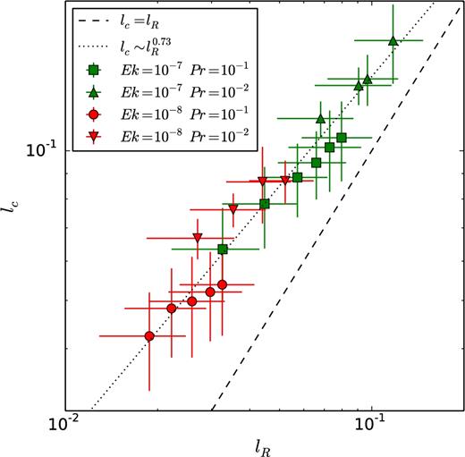
Convective lengthscale versus Rhines scale. Both quantities have been averaged radially in the inner convective region between 0.1 ≤ s ≤ 0.8. The horizontal and vertical bars indicate the standard deviation. The dotted line indicates the best fit to all the data points.
We now return to the issue of the interpretation of the velocity scale U in the Rhines scale formula (24). In our simulations, we find that the convective lengthscale approximately follows a power law lc ∼ U0.28 when U is interpreted as the r.m.s. total velocity. The power law exponent is therefore further away from the Rhines scale prediction when using the total velocity rather than the convective velocity.
3.3 Scaling of the zonal flow velocity
To complete this section, we now discuss how the amplitude of the zonal velocity scales with the convective velocity. Fig. 5(a) shows the evolution of the zonal Rossby number, Ro0 = Re0Ek, as a function of the convective Rossby number, Roc = RecEk, for Ek ∈ [10−8, 10−7] and Pr = [10−2, 10−1]. In this section we use the Rossby numbers to clarify the dependence of the velocity on the viscosity. For Ek Pr ≤ 10−9, the nonlinear onset of convection is subcritical (Guervilly & Cardin 2016). In this case, the zonal and convective Reynolds numbers are discontinuous and Rec ≳ 103. For each fixed value of Ek, the data points approximately fall on a straight line, indicating a power law dependence on Roc. The dashed line represents Ro0 = Roc. The data points cross this line for moderate values of the Rayleigh numbers that depend on the Prandtl number: at Ra ≈ 1.5Rac for Pr = 10−2 and Ra ≈ 6Rac for Pr = 10−1. The zonal flows have therefore large amplitude for relatively modest values of the Rayleigh numbers when Pr < 1, despite the presence of the Ekman boundary friction in our model. They reach an amplitude comparable to the amplitude of the convective flows for smaller Ra as Pr is decreased. In this sense, lower Pr is favourable for the zonal flows.

The power law (26) provides the closest exponent to our data best fit and is based on plausible physical arguments. By contrast, the power law (28) is too steep and the dependence of the pre-factor on Ek is much weaker in the data. The power law (27) requires a much stronger dependence of the convective lengthscale on Roc (namely |$l_c\sim \mbox{{Ro}}_c^{2/3}$|) than observed. Figs 5(b) and (c) show the dependence of Ro0 compensated by the power laws (26) and (27), respectively, on Roc. The data points compensated by the power law (26) align on a plateau, confirming that the exponent of this power law provides a reasonable agreement with our data.
The pre-factor of the power law (26) predicts that a decrease of Ek by a decade should lead to an increase of Ro0 by approximately a factor 3. The dependence on the Ekman number cannot be estimated accurately from our data points as they only sample one decade of Ek. Fig. 5(b) tentatively suggests that the power law (26) does not entirely explain the dependence on the Ekman number: in our simulations, Ro0 only increases by approximately a factor 2 when Ek decreases from 10−7 to 10−8.
4 DRIFT AND STABILITY OF THE ZONAL JETS
In the rest of the paper, we only consider simulations run at Ek = 10−8 and Pr = 10−1, where we obtain the largest number of zonal jets. The zonal flows have a strong influence on the convective flows, and hence on the heat transport as we will discuss in Section 6, so it is important to discuss the persistence of the zonal jets. In this section, we examine the stability of the jets.
Using a QG model of thermal convection, Rotvig (2007) shows that zonal jets drift inwards provided that the slope β has a significant dependence on radius, while QG models with constant β produce multiple jets that do not drift (e.g. Jones et al. 2003). Rotvig showed that the drift also occurs in a 3-D spherical model, so this effect is not restricted to QG models. The drift rate is found to increase with β and with the Rayleigh number. The drift of zonal flows is also observed in the rotating turntable experiment of Smith et al. (2014). In the experiment, β is positive and the drift is observed outwards. These studies thus indicate that the direction of the zonal jet drift is related to the sign of β.
Fig. 6 shows the space–time diagram of the zonal velocity for Ra/Rac = 0.96 and Ra/Rac = 9.02. For Ra = 0.96, the middle retrograde zonal jet drifts inwards periodically. In our system β < 0 so this inwards migration of the zonal flows is in agreement with the work of Rotvig (2007) and Smith et al. (2014).
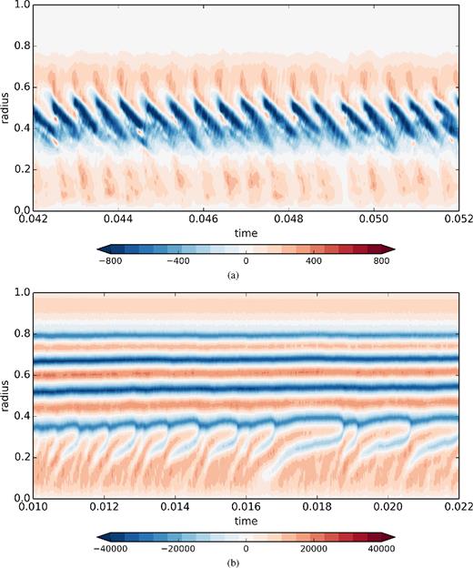
Space–time diagram of the zonal velocity for (a) Ra/Rac = 0.96 and (b) Ra/Rac = 9.02 (Ek = 10−8 and Pr = 10−1). The time interval corresponds to (a) 106 rotation periods and 317 convective turnover timescales (as defined in Table 1) and (b) 1.2 × 10⁶ rotation periods and 2672 convective turnover timescales.
For Ra/Rac = 9.02, the picture is completely different. For s > 0.4 the zonal jets do not drift and the standard deviation of their amplitude is of the order of 2000 (compared with a mean amplitude of approximately 30 000) over the course of the simulation. However at radius s < 0.4, the central prograde jet and its retrograde neighbour drift outwards. The retrograde jet initially forms around s = 0.2 and eventually merges with the retrograde jet located at s ≈ 0.35, closing off the prograde jet in the process. This sequence is not quite periodic and takes between 5 and 20 zonal turnover timescale (based on the time- and volume-averaged zonal velocity). The central region of the equatorial plane has the smallest values of β and dβ/ds, so the direction and the location of the drift indicates that this mechanism is different from the inward drift observed for smaller Ra and large β.
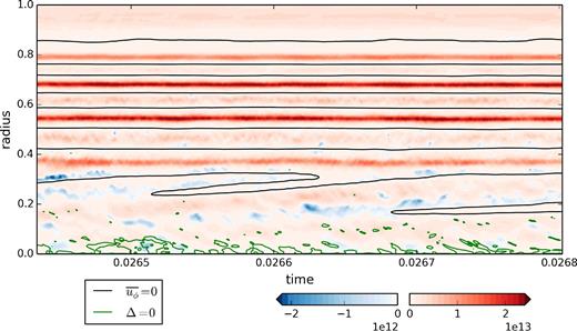
Space–time diagram of R (colour) for Ra/Rac = 9.02 (Ek = 10−8, Pr = 10−1). The isocontours |$\overline{u_{\phi }}=0$| and Δ = 0 have been represented in black and green, respectively. The time interval corresponds to 3.5 × 10⁴ rotation periods and 78 convective turnover timescales (as defined in Table 1).
5 DYNAMICAL DIFFERENCE BETWEEN RETROGRADE AND PROGRADE JETS
We now discuss the mechanism of formation of persistent zonal flows based on the extensive literature on the subject, particularly in the context of the ocean and atmosphere dynamics (e.g. Vallis 2006). In our simulations, retrograde zonal flows are faster and sharper than the rounded prograde zonal flows. This asymmetry is indicative of an important dynamical difference between the two types of zonal jets, related to their formation mechanism and to the sign of β. The asymmetry is also observed in 3-D models of rotating spherical convection (e.g. Heimpel & Aurnou 2007; Gastine et al. 2014) and in QG models with constant β (e.g. Teed et al. 2012). In the 3-D simulations, the multiple zonal jets emerge inside the tangent cylinder, where β is positive, so the prograde flows are faster and sharper than the retrograde flows.
The radial profile of the axisymmetric PV is plotted in Fig. 8 for Ra/Rac = 9.02. In the range s ∈ [0, 0.8], the succession of weak and steep PV gradient regions is visible and forms a relatively mild PV staircase for this value of Ra. Larger Ra are required to obtain well mixed PV regions and a better formed staircase profile. The asymmetry of the jets is clearly visible in our simulations but retrograde jets are not particularly narrower than the prograde jets. This is because the chosen delimitation of the jets (|$\overline{u_{\phi }}=0$|) is, somewhat arbitrarily, defined with respect to the planetary rotation. The profile of |$\overline{q}$| shows that the regions of steep PV gradients (which correspond to the cores of the retrograde jets) are in fact much narrower than the regions of weak PV gradients. Another characteristic of the zonal flow is the robustness of the prograde jet at the centre in all our simulations: this is well explained by the mixing in the central region that leads to a local increase of q. The PV mixing mechanism therefore provides a good explanation for the most notable features of the zonal flows observed in our simulations. Nevertheless, we note that alternative–although not mutually exclusive–mechanisms for the formation of persistent zonal flows have been put forward in the literature, such as resonant triad interactions (e.g. Pedlosky 1987).
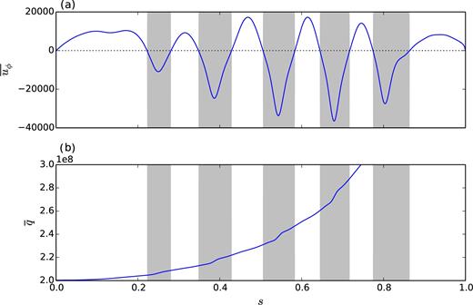
Radial profile of (a) the zonal velocity and (b) the axisymmetric potential vorticity (time averages) for Ra/Rac = 9.02 (Ek = 10−8, Pr = 10−1). The grey bands correspond to the regions where the zonal flow is retrograde.
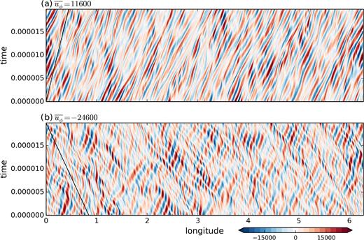
Hovmöller map (longitude–time) of the radial velocity us at a fixed radius: (a) s = 0.51 in a prograde jet (|$\overline{u_{\phi }}=11600$|) and (b) s = 0.58 in a retrograde jet (|$\overline{u_{\phi }}=-24600$|) for Ra/Rac = 6.44 (Ek = 10−8, Pr = 10−1). The solid black line shows the drift due to the advection by the zonal velocity. The time interval corresponds to 2000 rotation periods and 4 convective turnover timescales (as defined in Table 1).
We might expect that the dynamical difference between prograde and retrograde jets affects the temperature distribution because the Rossby waves might modify the transport properties of the flow. We study this problem in the next section.
6 EFFECT OF THE ZONAL FLOWS ON THE HEAT TRANSPORT
Fig. 10(a) shows these profiles for Ra/Rac = 9.02. The zonal flow (black line) is plotted according to the left axis and |$u_s^{\ast }$| (blue line) is plotted according to the right axis. Both profiles are time-averaged. In the inner convective region (s ≲ 0.8), the local maxima of |$u_s^{\ast }$| correlates well with the extrema of |$\overline{u_{\phi }}$| (the cores of the jets), that is, the zeros of the radial shear |$|\partial _s \overline{u_{\phi }}|$|, while the local minima of |$u_s^{\ast }$| correlates with maxima of |$|\partial _s \overline{u_{\phi }}|$| (the flanks of the jets). The reduction of |$u_s^{\ast }$| in the flank of a jet can reach 30 per cent of its value in the core of the neighbouring jets. The radial velocity is therefore impeded by the radial shear and maximized in the cores of jets, irrespective of their sign. Thus the dynamical difference between prograde and retrograde jets cannot be directly diagnosed on this profile.
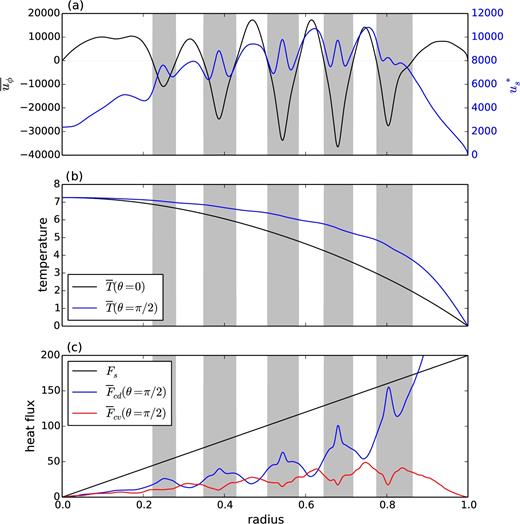
Radial profile of (a) the zonal velocity (black line) and the r.m.s radial velocity (blue), (b) the axisymmetric temperature along the rotation axis (black) and in the equatorial plane (blue), (c) the static heat flux (black), the conductive heat flux in the equatorial plane (blue) and the convective heat flux in the equatorial plane (red). All the quantities have been time-averaged. The grey bands correspond to the regions where the zonal flow is retrograde. The parameters are Ra/Rac = 9.02, Ek = 10−8 and Pr = 10−1.
To determine how the temperature field is affected by the zonal flows, Fig. 11(a) shows a meridional slice of the axisymmetric temperature, |$\overline{T}=\overline{\Theta }+T_s$|, averaged in time for the same simulation. The isotherms have an ellipsoidal shape which is elongated towards the equator. To complement this figure, the radial profiles of the axisymmetric temperature along the rotation axis, |$\overline{T}(\theta =0)$|, and in the equatorial plane, |$\overline{T}(\theta =\pi /2)$|, are plotted in Fig. 10(b). In the equatorial plane, the temperature has a flatter profile than along the rotation axis for s < 0.8, which explains the ellipsoidal shape of the isotherms. The thermal boundary layer is more pronounced in the equatorial plane. Nevertheless it remains thick (much thicker than the Ekman layer) because Pr < 1 and the Rayleigh number is moderate. The disparity between the temperature along the axial and equatorial directions is due to preferential direction of the convective flows in rapidly rotating convection. This effect is also observed in 3-D models (e.g. Zhang 1991; Yadav et al. 2016), but is amplified here by the use of a QG model.
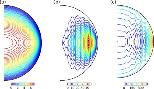
Meridional cross-section of the axisymmetric average of (a) the temperature |$\overline{T}=\overline{\Theta }+T_s$|, (b) the convective heat flux |$\overline{F}_{\text{cv}}$|, and (c) the conductive heat flux |$\overline{F}_{\text{cd}}$|. All the quantities have been time-averaged. Same parameters as Fig. 10.
On top of their ellipsoidal shape, the isotherms also have undulations of small amplitude. These undulations are located at the same distance from the rotation axis for each isotherm so they are likely due to the presence of zonal flows. This causal link is visible in Fig. 10(b) where we use the radial profile of |$\overline{T}(\theta =\pi /2)$| as a proxy for the z-averaged axisymmetric temperature. The temperature profile is relatively flat in the prograde zonal jets. By contrast it is significantly steeper in the core of the retrograde jets. This indicates that the mean temperature is affected by the PV distribution: in the core of the retrograde jets, the inhibition of the turbulence and the dominance of the Rossby waves imply that the temperature cannot be efficiently homogenized.
The thermal contrast between prograde and retrograde jets can be clearly observed in the profiles of the axisymmetric heat fluxes in the equatorial plane shown in Fig. 10(c). For comparison, the static heat flux Fs is also shown. Note that the profile of |$\overline{F}_{\text{cv}}$| and |$\overline{F}_{\text{cd}}$| at a given latitude are not representative of the spherical averages so their sum is not equal to Fs at each radius. The local maxima of the convective flux are located in the prograde zonal jets. The decrease of the convective flux matches the decrease of |$u_s^{\ast }$| in the shear layers. However the convective flux systematically reaches minima in the core of the retrograde jets while the radial velocity recovers there. The conductive flux is boosted in the shear layers, but even more so in the retrograde jets, where it is much larger than the convective flux. The balance between the thermal processes is very different in the prograde and retrograde jets: the prograde jets are regions where about half of the heat is carried by the convection and the temperature is fairly uniform, whereas most of the heat is carried by the conductive flux in the retrograde jets. This occurs despite high values of the r.m.s radial velocity in the retrograde jets, so the radial flow must not be well correlated with the temperature perturbation in these regions. Fig. 12 show the Hovmöller map for the non-axisymmetric temperature perturbation, |$\Theta ^{\prime }=\Theta -\overline{\Theta }$|, for the same parameters and radius as Fig. 9. In both prograde and retrograde jets, the temperature perturbation drifts in the direction of the zonal flow with a drift rate consistent with the advection by the zonal velocity. In the core of the retrograde jets, which are dominated by the propagation of Rossby waves, the radial velocity and temperature perturbation are visibly not well correlated. The inefficiency of the Rossby waves at transporting heat outwards explains the weak convective heat flux there. In the prograde jet, Θ΄ is well correlated with us, which is consistent with the high convective heat flux.
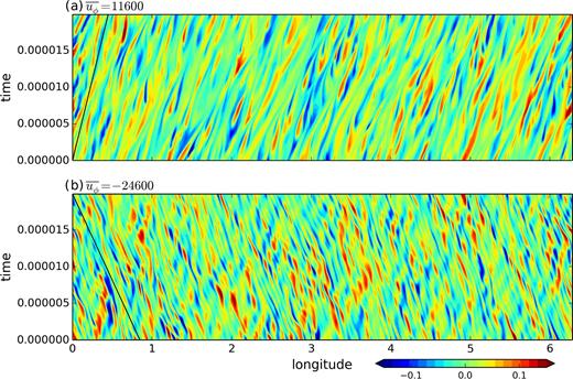
Hovmöller map of the non-axisymmetric temperature perturbation, Θ΄, at a fixed radius: (a) s = 0.51 in a prograde jet and (b) s = 0.58 in a retrograde jet for the same parameters as Fig. 9. The solid black line shows the drift due to the advection by the zonal velocity. The time interval corresponds to 2000 rotation periods and 4 convective turnover timescales (as defined in Table 1).
In summary, our results show that the core of the retrograde jets—and not only the regions of intense shear—act as primary bottlenecks to the convective heat transport.
7 DISCUSSION
In this paper, we have studied the convective structures and zonal flows that form in rotating thermal convection for values of the Prandtl number relevant for liquid metals (|$\mbox{{Pr}}=\mathcal {O}(10^{-1})$|) and low Ekman (|$\mbox{{Ek}}=\mathcal {O}(10^{-8})$|) and Rossby numbers (Roc < 10−2). In order to reach low values of the Ekman number, we have used a hybrid numerical model that couples a QG approximation for the velocity to a 3-D temperature field. Convection is driven by internal heating in a full sphere geometry. The model includes Ekman pumping to mimic no-slip boundary conditions. We focus on the intense zonal flows that emerge on the strong branch of convection, which was described by Guervilly & Cardin (2016) using the same hybrid QG-3D model and by Kaplan et al. (2017) in a fully 3-D model. Persistent multiple zonal jets of alternating sign form due to the mixing of PV and exert a strong feedback on the convection. An upscale energy transfer takes place and the integral convective lengthscale increases with the vigour of the convection. The convective lengthscale and the zonal jet width are closely related: the radial shear exerted by the zonal flow on the radial velocity limits the size of the convective eddies, while the typical mixing length of the PV depends on the size of the most energetic convective eddies. The convective lengthscale varies radially in agreement with the Rhines scale (Rhines 1975), that is, as the square root of β, where β measures the slope of the boundaries. However the convective scale increases more slowly with the convective speed (following a power law of exponent 0.37) than predicted by the Rhines scale (power law of exponent 0.5).
In our QG model, convection carries heat mostly in the direction perpendicular to the rotation axis. We have shown that the principal barrier to this convective heat transport is located in the cores of the retrograde zonal jets. This is due to the formation of a staircase of PV: steep and weak gradients of the PV correspond to retrograde and prograde zonal jets, respectively. The steep PV gradients inhibit the eddies and favour the propagation of Rossby waves, which are inefficient at carrying heat outwards. The occurrence of eddy-transport barriers associated with strong zonal jets is well-documented in the atmospheric dynamics context (Dritschel & McIntyre 2008). In our simulations, these barriers lead to the steepening of the mean temperature gradient in the core of the retrograde jets, and there, the heat is largely carried by conduction. The unfavourable effect of the shear layer in the flanks of the zonal jets on the convective heat transport is secondary by comparison. To illustrate the thermal signature of the retrograde jets at the surface, we plot in Fig. 13 the latitudinal profile of the axisymmetric heat flux at r = 1. The most noticeable feature is that the heat flux is maximal at the equator, which is expected as the convective transport is largely perpendicular to the rotation axis, and is also observed in 3-D models (e.g. Zhang 1991; Yadav et al. 2016). This enhanced heat transport in the equatorial regions compared with the polar regions is used in a number of models of the Earth's inner core growth to explain the observed seismic anisotropy (e.g. Yoshida et al. 1996; Deguen & Cardin 2009). Of greater interest here are the more subtle variations of the surface heat flux at higher latitudes: the cores of the retrograde jets are characterized by local maxima of the (conductive) surface heat flux. This occurs because the axisymmetric temperature gradient is steepest in these regions. To highlight the small-scale anomalies of the surface heat flux and quantify their amplitude, we filter out the coefficients of the spherical harmonics of degree l smaller than 30. The filtered profile is plotted according to the right axis of Fig. 13 in blue. It shows that the heat flux anomalies due to the presence of the zonal flows are sharp and of a small amplitude, approximately 1 per cent of the mean surface heat flux. The thermal signal associated with zonal jets provides useful information in the context of the gas giant planets because the power emitted at the surface of the planet can be measured. For Jupiter and Saturn, the emitted power is approximately uniform in latitude with variations of small amplitude that resemble the structure of the zonal flows at the surface (Pirraglia 1984; Li et al. 2010).
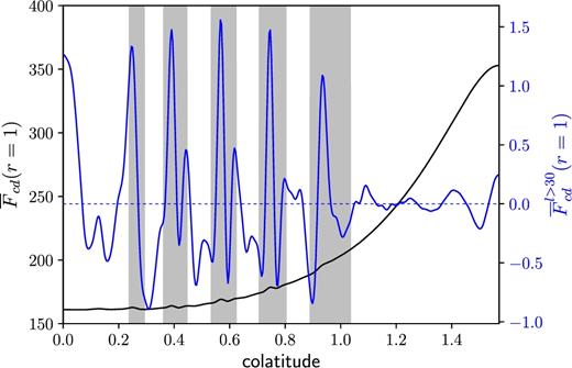
Latitudinal profile of the axisymmetric heat flux (black line) from the North pole to the equator at the outer boundary r = 1 for Ek = 10−8, Pr = 10−1 and Ra/Rac = 9.02. The blue line shows the axisymmetric heat flux where the spherical harmonics coefficient of degrees l ≤ 30 have been filtered out and is plotted according to the right axis. The grey bands correspond to the regions where the zonal flow is retrograde.
For increasing thermal driving (out of reach of our current computational resources), we expect the convective eddies to further enhance the mixing of PV in the prograde jets. The PV staircase would then become sharper with narrower regions of steep PV gradients, and hence narrower retrograde jets. This sharpening of the PV staircase in rapidly rotating convection is observed by Verhoeven & Stellmach (2014) at large Rayleigh numbers (20 times supercritical) in 2-D numerical simulations using the anelastic approximation. In their study, the β effect is due to the compressibility of the fluid (Ingersoll & Pollard 1982; Glatzmaier et al. 2009) and leads to the formation of multiple zonal jets, similarly to the topographic β effect as studied here. They show that the sharpening of the PV staircase results in the sharpening of the entropy staircase (analogous to the temperature staircase in the Boussinesq approximation). In QG systems with vigorous convection, we thus expect the heat transport process to be heterogeneous with wide convective regions separated by narrow conducting bands; the efficiency of the heat transfer throughout the whole system would largely be controlled by the efficiency of the conducting process across the retrograde jets, and thus, by the width of these conducting bands. This process is partly analogous to the occurrence of layering in double-diffusive convection where the heat transfer is controlled by the flux through the interface between overturning layers (Turner 1985).
The main features of the nonlinear QG dynamics discussed in this paper do not crucially rely on the temperature being 3-D. Consequently, we expect that QG models of rotating convection using a 2-D temperature field would be able to reproduce our observations qualitatively. QG-2D models could be used to pursue this study at lower Ekman numbers and larger Rayleigh numbers. The numerical framework used in the hybrid QG-3D model is however well suited to explore the possible existence of dynamos driven by QG flows at low magnetic Prandtl numbers (e.g. Gillet et al. 2011). The dynamo problem indeed requires to treat the magnetic field in 3-D. We shall investigate QG dynamos in a forthcoming study.
Acknowledgements
CG was supported by the Natural Environment Research Council under grant NE/M017893/1. PC acknowledges the Agence Nationale de la Recherche for supporting this project under grant ANR TuDy. This work was undertaken on TOPSY of the HPC facilities at Newcastle University and on the facilities of N8 HPC Centre of Excellence, provided and funded by the N8 consortium and EPSRC (Grant EP/K000225/1) and coordinated by the Universities of Leeds and Manchester. We are grateful to the referees for helpful comments that improved the manuscript.
REFERENCES
