Deformation rates in northern Cascadia consistent with slow updip propagation of deep interseismic creep

Bruhat, Lucile; Segall, Paul

doi:10.1093/gji/ggx317

Abstract

Interpretations of interseismic slip deficit on the northern Cascadia megathrust are complicated by an enigmatic ‘gap’ between the downdip limit of the locked region, inferred from kinematic inversions of deformation rates, and the top of the episodic tremor and slip (ETS) zone. Recent inversions of global positioning system (GPS) and tide gauge/leveling data for shear stress rates acting on the megathrust found a ∼21 km locking depth with a steep slip-rate gradient at its base is required to fit the data. Previous studies have assumed the depth distribution of interseismic slip rate to be time invariant; however, steep slip-rate gradients could also result from the updip propagation of slip into the locked region. This study explores models where interseismic slip penetrates up into the locked zone. We consider the creeping region, corresponding to the gap and the ETS zone, as a quasi-static crack driven by the plate velocity at its downdip end. We derive a simple model that allows for crack propagation over time, and provides analytical expressions for stress drop within the crack, slip and slip rate on the fault. It is convenient to expand the non-singular slip-rate distribution in a sum of Chebyshev polynomials. Estimation of the polynomial coefficients is underdetermined, yet provides a useful way of testing particular solutions and provides bounds on the updip propagation rate. When applied to the deformation rates in northern Cascadia, best-fitting models reveal that a very slow updip propagation, between 30 and 120 m yr⁻¹ along the fault, could explain the steep slip-rate profile, needed to fit the data. This work provides a new tool for estimating interseismic slip rates, between purely kinematic inversions and full physics-based modeling, allowing for the possibility for updip expansion of the creeping zone.

Creep and deformation, Seismic cycle, Transient deformation, North America, Mechanics, theory, and modelling

1 INTRODUCTION

While we are periodically reminded that megathrust earthquakes are the most damaging events along coastal margins, hazard assessment remains complex. Earthquake hazard assessment rests in particular on the size of the rupture zone and its distance to onshore population centers. The former impacts directly the earthquake magnitude, as the seismic moment is proportional to rupture area. The latter is controlled, in subduction zones, by the maximum depth of the earthquake, since, due to the obliqueness of the fault interface, a deeper rupture means larger slip close to land. Inversions of interseismic geodetic deformation rates provide an estimate of the locked part of the megathrust, whose downdip limit is referred to as the locking depth. Below this, the fault slips aseismically, and may not accumulate elastic strain. The locking depth is then commonly considered as a proxy for the maximum rupture depth. Nevertheless, it only reveals a lower bound for the maximum rupture area. Forecasts of locking depth have been invalidated by actual rupture records as observed during the 2011 Tohōku megatrust (e.g. Ide et al. 2011), or the 2015 Gorkha earthquake (Avouac et al. 2015). In both examples, the estimated depth of the earthquake rupture extended below the locking depth inferred by kinematic inversions. These inversions also only provide a snapshot of the slip rate, without any information on stress state on the megathrust. In particular, the nature of the downdip extent of the locked region is often neglected. Due to downdip loading, stress accumulates most rapidly in the vicinity of the locking depth, making this region most likely to nucleate earthquakes. Therefore, hazard assessment in megathrust regions would benefit from a better understanding of the mechanical processes in the vicinity of the locking depth.

The simplest 2-D models of interseismic deformation consider a single dislocation, with the fault locked to some depth, but slipping steadily below (e.g. Savage & Burford 1970). Using this simplified model, kinematic inversions of surface deformation rates have, for decades, been used to estimate the locking depth, presumed to delimit the deep extent of the seismogenic region. More realistic models involve some smoothing of the locked to creeping transition, but almost all kinematic inversions assume that the slip-rate distribution is stationary in time. More physically motivated models are exceptions (e.g. Johnson & Segall 2004; Takeuchi & Fialko 2012; Hearn & Thatcher 2015). Recently, numerical physics-based earthquake cycle simulations have called the assumption of a stationary interseismic slip-rate profile into question. Noting the absence of microseismicity at the base of the Carrizo Plain segment of the San Andreas Fault, Jiang & Lapusta (2016) proposed that strong dynamic weakening promotes seismic rupture into the velocity-strengthening region, deepening the locked-creeping transition. During the interseismic period, this transition slowly migrates upward over time. As creep penetrates into the locked region, a stress concentration builds at the velocity weakening/strengthening transition, possibly triggering earthquakes there. Similar behaviour has been observed with quasi-dynamic simulations including thermal pressurization (Segall & Bradley 2012), where slow slip events (SSEs) gradually propagate into the locked zone between megathrust events. Even conventional rate-state friction fault models, without strong dynamic weakening, exhibit upward penetration of the locked to creeping transition, over lengths that scale with the critical slip weakening distance d_c.

In this study, we explore this hypothesis to explain the deep interseismic slip-rate distribution in Northern Cascadia. The Cascadia subduction zone is known to host M_w ∼ 9 megathrust events (Atwater 1987; Satake et al. 1996; Goldfinger et al. 2003; Satake 2003); however, due to the lack of direct observations, little is known about the characteristics of these events. The downdip extent of a future rupture remains an open question. An upper bound for the locking depth in Cascadia is often suggested by the presence of SSEs, accompanied by tremors and low-frequency earthquakes, known as episodic tremor and slip (ETS), at depths between ∼30 and 40 km (Wech et al. 2009; Holtkamp & Brudzinski 2010; Bartlow et al. 2011; Wech & Bartlow 2014). In fact, observations from the Nankai region in Japan (Obara 2011) have noted that the ETS zone seems to delimit the downdip extent of previous megathrust earthquakes. In Cascadia, kinematic inversions of geodetic data have estimated the locking depth to be between 12 and 20 km (Hyndman & Wang 1995; Flück et al. 1997; McCaffrey et al. 2007; Burgette et al. 2009), leading to an enigmatic ‘gap’ between the bottom of the locked region and top of the ETS zone (Dragert et al. 2004; McCaffrey et al. 2007; Wech & Creager 2011; Hyndman 2013; McCaffrey et al. 2013). Special attention is given to the gap because its existence complicates estimations of the depth extent of future megathrust earthquakes, which might rupture either to the bottom of the fully locked region, between 12 and 20 km, or to the top of the ETS zone at 30 km.

Recent work by Bruhat & Segall (2016) investigated the characteristics of the gap by combining analysis of long-term deformation rates and physics-based modeling to determine how interseismic slip deficit accumulates on the megathrust. They implemented rate-state friction models of SSEs to match the average SSE displacements in Cascadia. These models predicted roughly constant shear stress on the megathrust within the SSE zone when averaged over many SSE cycles. That is, stress accumulates between SSE and is then released by slow slip. Yet, when the fault is locked to the top of the ETS zone, the same models misfit the data, especially the uplift rates, predicting too much interseismic locking when compared to decadal-averaged surface velocities. They showed that neither heterogeneous Green's functions nor velocity-strengthening friction within the gap could explain the observations. Using inversions that sought interseismic slip rates as close as possible to the physics-based models, they demonstrated that faster slip rates, relative to the rate-state-dependent models, are required within both the gap and the ETS zone. As an intermediate step between kinematic inversions and fully physics-based predictions, they inverted for shear stress rates on the megathrust and showed that negative shear stress rates within both the gap and the ETS region, up to 2.5 kPa yr⁻¹ at a depth of 25 km, and deep locking depths, around 21 km, are required to fit the data. Their work revealed a discrepancy between physics-based predictions, which suggest no change in shear stress within the ETS region and the data-driven results that require high slip rates, implying decreasing shear stress on the fault within the gap and the ETS region.

Like most kinematic inversions of geodetic surface rates, Bruhat & Segall (2016) assumed the locking depth, and thus the depth distribution of interseismic fault slip rate, to be time invariant. However, high interseismic slip rates in the gap could also result from the updip propagation of slip into the locked region. Consider the interseismic slip distribution as a crack (not necessarily of constant stress) of length a driven from below by steady creep at long-term rate v^∞. Slip is defined in terms of the deep displacement v^∞t, and a depth-dependent function f (z, t):

\begin{eqnarray} s(z,t) = f(z,t)v^{\infty }t. \end{eqnarray}

(1)

The instantaneous slip rate is

\begin{eqnarray} \frac{d s}{d t}(z,t)&=& f(z,t)v^{\infty } + v^{\infty }t\frac{\partial f}{\partial t} \nonumber \\ &=& f(z,t)v^{\infty } + v^{\infty }t\frac{\partial f}{\partial a}\frac{\partial a}{\partial t}. \end{eqnarray}

(2)

Only if the shape function f (z, t) is time invariant is the slip rate also time invariant, ds/dt = f (z)v^∞. More generally, propagation of the creeping zone, ∂a/∂t, leads to an additional term in the slip rate, which has been mostly neglected in kinematic slip-rate inversions. Such a model might provide a physical mechanism to explain the faster slip rates, relative to the physics-based solutions, required to fit geodetic observations in Cascadia, and help reconcile inversion predictions with numerical modeling.

In the present work, we investigate models where interseismic slip penetrates updip into the locked region, over time-scales that are long compared to ETS recurrence times. That is we do not consider the ETS events themselves. The ETS zone and gap is modeled as a quasi-static crack driven by plate motion at the fixed downdip limit of the ETS region. Following classical crack models of faults, we present a simple model that allows crack growth over time, and derive analytical expressions for stress drop within the crack, slip and slip rate along the fault. It proves convenient to expand any non-singular slip-rate distribution in a combination of Chebyshev polynomials. The decomposition in polynomials leads to a severely underdetermined problem. However, it allows us to test particular solutions, such as those that provide bounds on the possible updip propagation rate, or that optimize inferred characteristics of the slip and stress distributions. When applied to observed deformation rates in Cascadia, best-fitting models reveal that a very slow updip propagation is consistent with the data, and offers a physically plausible explanation for the negative shear stress rates observed in our previous study (Bruhat & Segall 2016).

2 METHODS

2.1 Crack models for penetrating creep

In this section, we describe the model for deep interseismic creep as a long-term quasi-static crack driven by steady downdip plate motion. Following classical crack models of faults, we present a simple model that allows crack growth over time, and derive analytical expressions for stress drop within the crack, slip and slip rate along the fault. We describe here the main results of the derivation; the full derivation is given in Appendix A.

Consider a 1-D mode II crack of length a, lying on the fault surface and loaded at constant long-term slip rate v^∞ at depth z = 0 (Fig. 1). The medium is loaded by remote shear stress τ^∞, uniform in time, but not necessarily in space. The crack slips at stress τ, such that the stress drop is defined as Δτ = τ^∞ − τ. Consider the spatial variables ξ and z such that ξ ∈ [−1, 1] and z ∈ [0, a]; the mapping between ξ and z, such that the end z = 0 is fixed during crack growth, is:

\begin{eqnarray} \xi &=& 1-\frac{2z}{a}. \end{eqnarray}

(3)

In a full space, the relation between the Burger's vector distribution B(ξ) ≡ ∂s/∂ξ, where s is fault slip, and the spatially variable stress drop within the crack Δτ is

\begin{eqnarray} B(\xi ) = -\frac{2(1-\nu )}{\mu \pi }\int _{-1}^{1} \frac{\Delta \tau (u) \sqrt{1-u^2}}{(\xi -u)\sqrt{1-\xi ^2}} du+ \frac{2 A}{a\sqrt{1-\xi ^2}} \end{eqnarray}

(4)

(Bilby & Eshelby 1968), where A is a constant proportional to the net dislocation, μ the shear modulus and ν Poisson's ratio. Note that this formulation excludes free-surface effects, which will be considered in an ensuing section.

Figure 1.

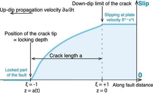
Interseismic slip rate modeled as a crack of size a(t) driven by constant downdip displacement δ^∞ = v^∞t. During crack growth, the shallow limit of the crack, here the locked-to-creeping transition depth, migrates updip.

Open in new tab Download slide

Following Bilby & Eshelby (1968) [see also Segall (2010, chap. 4)], the integration for B(ξ) can be conveniently performed by decomposing the stress drop within the crack in Chebyshev polynomials of the first kind T_i

\begin{eqnarray} \Delta \tau (u) = \frac{\mu }{1-\nu } \sum _{i=0}^{\infty } c_i T_i(u). \end{eqnarray}

(5)

Solving eq. (4) for a non-singular crack, that is, with finite stress at the crack tip, z = a(t), and driven by steady displacement v^∞t relates

\begin{eqnarray} A &=& \frac{v^{\infty }t}{\pi }, \end{eqnarray}

(6)

and yields

\begin{eqnarray} \Delta \tau (\xi ,t)&=& \frac{\mu }{1-\nu } \frac{2v^{\infty } t}{a\pi } \xi + \frac{\mu }{1-\nu } \sum _{i=2}^{\infty } c_i T_i(\xi ), \end{eqnarray}

(7)

\begin{eqnarray} B(\xi ,t) &=& \frac{4 v^{\infty }t}{a\pi }\sqrt{1-\xi ^2}+2\sqrt{1-\xi ^2}\sum _{i=2}^{\infty } c_i U_{i-1}(\xi ), \end{eqnarray}

(8)

where U_i are Chebyshev polynomials of the second kind. Integrating the Burger's vector distribution, to obtain the fault slip yields

\begin{eqnarray} s(\xi ,t) &=& \frac{v^{\infty }t}{\pi }\Bigg [\xi \sqrt{1-\xi ^2} + \arcsin (\xi ) + \frac{\pi }{2}\Bigg ] +\frac{a}{2}\sqrt{1-\xi ^2}\sum _{i=2}^{\infty }c_i\Bigg [\frac{U_{i}(\xi )}{i+1} -\frac{U_{i-2}(\xi )}{i-1}\Bigg ]. \end{eqnarray}

(9)

Finally, taking the total derivative of s(ξ, t) to get slip rate, we find

\begin{eqnarray} \frac{ds}{dt}(\xi ,t) &=& v^{\infty }g+ \frac{a}{2} \sum _{i=2}^{\infty }\frac{d c_i}{d t} f_{i} + \frac{d a}{d t} \Bigg [g^{\prime }\frac{1-\xi }{a}v^{\infty }t+ \sum _{i=2}^{\infty }\frac{c_i}{2} \Big (f_{i} + f_i^{\prime }(1-\xi )\Big )\Bigg ], \end{eqnarray}

(10)

where

\begin{eqnarray} f_i &=& \sqrt{1-\xi ^2}\Bigg [\frac{U_{i}}{i+1} -\frac{U_{i-2}}{i-1}\Bigg ], \end{eqnarray}

(11a)

\begin{eqnarray} f^{\prime }_i &=& 2\sqrt{1-\xi ^2}U_{i-1}, \end{eqnarray}

(11b)

\begin{eqnarray} g &=& \frac{1}{\pi }\Bigg [\xi \sqrt{1-\xi ^2} + \arcsin \xi + \frac{\pi }{2}\Bigg ], \end{eqnarray}

(11c)

\begin{eqnarray} g^{\prime } &=& \frac{2}{\pi }\sqrt{1-\xi ^2}. \end{eqnarray}

(11d)

Note that using eq. (10) one can expand any non-singular slip-rate distribution in a combination of Chebyshev polynomials, with i > 1. We also derive an expression for the stress drop rate:

\begin{eqnarray} \frac{d\Delta \tau }{dt}&=&\frac{\mu }{1-\nu }\frac{ 2v^{\infty }}{\pi a}\xi + \frac{\mu }{1-\nu } \sum _{i=2}^{\infty } \frac{d c_i}{dt} T_i(\xi )+ \frac{\mu }{1-\nu }\frac{\dot{a}}{a}\Bigg [\frac{2 v^{\infty }t}{\pi a}(1-2\xi )+ (1-\xi )\sum _{i=2}^{\infty } c_i iU_i\Bigg ]. \end{eqnarray}

(12)

When comparing to observations, we consider the following to be unknown: the size of the creeping region a, the propagation velocity |$\dot{a} \equiv da/dt$|⁠, the age of the crack, or loading time, t, the coefficients of the Chebyshev polynomials c_i and their time derivatives dc_i/dt. This is a severely underdetermined problem, as are most geodetic inversions. However, this formulation allows us to test particular solutions, such as in the following sections.

2.2 First-order description

In this section, we examine the simplest case where for all i > 1, c_i = 0 and dc_i/dt = 0. This simplification leads to the following stress drop, stress drop rate, slip and slip-rate distributions:

\begin{eqnarray} \Delta \tau (\xi ,t) &=& \frac{\mu }{1-\nu } \frac{2v^{\infty } t}{a\pi } \xi , \end{eqnarray}

(13a)

\begin{eqnarray} \frac{d\Delta \tau }{dt}&=& \frac{\mu }{1-\nu }\frac{2v^{\infty }}{\pi a}\Bigg [\xi + \frac{\dot{a}t}{a}(1-2\xi )\Bigg ], \end{eqnarray}

(13b)

\begin{eqnarray} s(\xi ,t) &=& \frac{v^{\infty }t}{\pi }\Bigg [\xi \sqrt{1-\xi ^2} + \arcsin (\xi ) + \frac{\pi }{2}\Bigg ], \end{eqnarray}

(13c)

\begin{eqnarray} \frac{ds}{dt}(\xi ,t) &=& \frac{v^{\infty }}{\pi }\Bigg [\xi \sqrt{1-\xi ^2} + \arcsin (\xi ) + \frac{\pi }{2}\Bigg ] + \dot{a}\frac{2v^{\infty }t}{a\pi }(1-\xi )\sqrt{1-\xi ^2}. \end{eqnarray}

(13d)

For a stationary crack, |$\dot{a}$| = 0, the shape of slip-rate distribution is the same as the slip profile. Fig. 2 displays slip rate, cumulative slip, stress within the crack τ – τ^∞ = −Δτ, and stress rate profiles at different times for a crack propagating at 40 m yr⁻¹ along depth. Allowing the crack to grow pushes the locked-creeping transition upward from 20 to 14 km in 150 yr. Over time, the slip-rate profile steepens due to the increasing contribution of the second term in the slip-rate eq. (13d). Fig. 2 shows that, while the slip-rate transition might be abrupt, there could be significant slip deficit below this point. This has important consequences for the slip deficit along a fault segment, traditionally interpreted solely in terms of the current slip-rate distribution. Note that the stress at the crack tip increases as the crack propagates into the locked region. Stress rate is positive in the region above 22 km before propagation. As the crack grows, stress rates become more negative, in particular close to the tip. In eq. (13b), this is caused by the increasing weight with time of the propagation term.

Slip-rate, cumulative slip, stress τ – τ∞ = −Δτ and stress rate profiles at different times for a crack propagating upward at 40 m yr−1. These profiles are derived using eqs (13a)–(13d), at t from 0 to 150 yr for a crack driven by constant slip rate below z = 25 km.

Figure 2.

Slip-rate, cumulative slip, stress τ – τ^∞ = −Δτ and stress rate profiles at different times for a crack propagating upward at 40 m yr⁻¹. These profiles are derived using eqs (13a)–(13d), at t from 0 to 150 yr for a crack driven by constant slip rate below z = 25 km.

Open in new tab Download slide

Fig. 3 shows how the propagation speed affects the slip-rate profile, in particular the steepness of the locked-to-creeping transition. Here we present slip rate, cumulative slip, stress within the crack and stress rate profiles at the same time (t = 150 yr) for a crack propagating upward at various speeds. Since neither the slip nor stress profiles depend on the propagation speed, all profiles are the same. However, faster propagation results in increasing steepness of the slip-rate profile at the downdip end of the fully locked region. Increasing the updip velocity also leads to more negative stress rates, that is, larger stress reduction, in the shallow part of the crack.

Slip-rate, cumulative slip, stress τ – τ∞ = −Δτ and stress rate profiles at propagation speeds from 0 to 40 m yr−1. These profiles are derived using eqs (13a)–(13d), at t = 150 yr for a crack driven by constant slip rate below z = 25 km.

Figure 3.

Slip-rate, cumulative slip, stress τ – τ^∞ = −Δτ and stress rate profiles at propagation speeds from 0 to 40 m yr⁻¹. These profiles are derived using eqs (13a)–(13d), at t = 150 yr for a crack driven by constant slip rate below z = 25 km.

Open in new tab Download slide

We next investigate whether this model can explain the long-term rates in northern Cascadia.

3 APPLICATION TO NORTHERN CASCADIA

3.1 Deformation rates

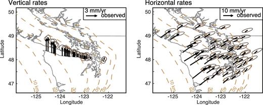
This study considers decadal-averaged deformation rates, referred here as ‘long term’, in the Olympic Peninsula–southern Vancouver Island region collated in Bruhat & Segall (2016) and displayed in Fig. 4. Horizontal rates were computed from GPS positions measurements (from the PANGA network solutions from Central Washington University), spanning eight SSEs, from 2000 to mid-2015. GPS vertical velocities are ignored in this study because of their large uncertainties. We also analyse uplift rates from tide gauges and leveling surveys from the early 1930s in the northern Washington area along the Strait of Juan de Fuca and on the East side of the Puget Sound compiled in Krogstad et al. (2016). These rates were corrected for present-day uplift rates due to post-glacial rebound (James et al. 2009) and assume zero vertical motion at the Seattle tide gauge, consistent with regional sea level reconstructions (Burgette et al. 2009). Due to uncertainty in that last assumption, we solve for a free parameter α that allows the uplift rates to translate uniformly in the inversions.

Figure 4.

Data sets used in this study, collated in Bruhat & Segall (2016). Left: uplift rates derived from tide gauges and leveling measurements. Horizontal gobal positioning system (GPS) velocities computed from daily positions between 2000 and 2015. Right: uncertainties correspond to the 95 per cent confidence intervals.

Open in new tab Download slide

Although Bruhat & Segall (2016) assumed the long-term rates to be statistically independent, spatial correlations are well known in geodetic data (e.g. Gudmundsson et al. 2002; Mavrommatis et al. 2015). In this study, we empirically estimate the correlations in the velocities to populate the full covariance matrix (see details in Appendix B). Large correlation lengths in the horizontal GPS measurements, compared to those in the uplift rates are inferred, which naturally decreases the weight of the GPS data in later inversions.

3.2 Slip-rate inversions

In this section, we apply the model for a non-singular quasi-static crack derived in Section 2 to the long-term deformation rates observed in Northern Cascadia. As mentioned in the previous section, this problem is severely underdetermined. We will then consider end-member cases to determine which model seems more appropriate to describe long-term deformation in Cascadia.

Surface velocities d = [d_horz ; d_vert] are related to fault slip rates |$\mathbf {\dot{s}} \equiv \mathbf {d s/dt}$| via:

\begin{equation} {\left[\begin{array}{cc}\mathbf {d_{horz}} \\ \mathbf {d_{vert}} \\ \end{array}\right]} = \mathbf {G} \mathbf {\dot{s}} + \alpha {\left[\begin{array}{cc}\mathbf {0} \\ \mathbf {1} \\ \end{array}\right]} + \epsilon \quad \textrm{with} \quad \epsilon \sim \mathcal {N}(0,\mathbf {\Sigma }). \end{equation}

(14)

where G are homogeneous half-space Green's functions, |$\mathbf {\dot{s}}$| is the unknown vector of slip rates, Σ is the data covariance matrix and α a parameter that accounts for the uncertainties in the reference frame for vertical motion. From eq. (10), |$\mathbf {\dot{s}}$| is uniquely specified by: the crack length a, the loading time t, the propagation rate |$\dot{a}$|⁠, the coefficients of the Chebyshev polynomials c_i and their time derivatives dc_i/dt.

The inverse problem is the following: we aim to estimate at least the size of the crack a and α. The inferred a also provides the updip limit of the crack, or locking depth, since we fix the downdip limit of the crack at the base of the ETS region, at a depth of 40 km. Depending on the case, we potentially also invert for |$\dot{a}$|⁠, t, the c_i and their derivatives dc_i/dt. We employ Markov Chain Monte Carlo (MCMC) methods for the inversions. We found MCMC algorithms to be an attractive choice, as they efficiently estimate the maximum-likelihood solution and also enable the construction of posterior distributions. We assume no prior knowledge about the model parameters, except for t. The loading time t corresponds to the age of the crack, that is, to the time it started to propagate. Therefore, t ranges between the age of the oldest uplift measurements we invert for (80 yr) and the time of the last megathrust event (315 yr). Note that this definition of t assumes that slip processes including the rate of propagation have been constant in time, although there is no expectation that this is the case in nature. Moreover, because vertical data are averaged over 80 yr, they do not provide significant temporal resolution. As a result, t should not necessarily coincide with time since last megathrust event.

To compare model predictions with data, we follow the pseudo 3-D approach of Bruhat & Segall (2016). The crack model provides a 1-D, along-fault profile of long-term slip rate, that is then draped over the plate boundary geometry of McCrory et al. (2012). This yields a 2-D slip-rate distribution, which allows us to predict deformation rates at the Earth's surface, but does not account for along-strike heterogeneity or slip-rate variations due to non-planarity of the plate boundary.

3.3 Free-surface effects

The relations between slip and stress in Section 2 are only fully valid in a full space. The free-surface results in an extra, non-singular, term K(u, ξ) in the relationship between stress drop Δτ and the Burger's vector distribution B:

\begin{eqnarray} \Delta \tau (u) = \frac{\mu }{2\pi (1-\nu )}\int _{-a/2}^{a/2} B(\xi )\Bigg [\frac{1}{(u-\xi )}+K(u,\xi )\Bigg ] d\xi . \end{eqnarray}

(15)

The kernel K(u, ξ) depends on the fault position relative to the free surface. Analytic solutions to eq. (15) are generally not possible (e.g. Erdogan & Gupta 1972; Hills et al. 1996). Numerical procedures have been developed to invert this equation (Erdogan & Gupta 1972), but require specification of the stress drop distribution. Since one of our goals in this study is to infer the state of stress acting on the fault, we cannot follow this procedure.

It is still convenient to expand the slip, and slip-rate, distributions in Chebyshev polynomials. The relationship between slip rate and surface displacement rate, G in eq. (14), is computed using a boundary element method (BEM) including the free-surface contribution. Similarly, we employ BEM-based elastic Green's functions to compute the stress and stress-rate acting on the fault, which similarly account for the free surface. Fig. 5 displays slip-rate distributions for two crack models derived using the first-order description (eqs 13a–13d). The first model corresponds to a stationary crack, that is, |$\dot{a}$| = 0, whereas the second model describes a crack propagating at 40 m yr⁻¹ along the fault. Stress rate profiles computed from eq. (13b) and by BEM are compared. The BEM approach, which includes free-surface effects, depends on the fault dip, taken here to be 8° (inferred from McCrory et al. 2012). As expected, for both slip rates, the corresponding stress rate profiles, computed using eq. (13b), present larger amplitude than the stress rate including the free surface. To account for the free-surface effects, the inferred stress and stress rate distributions in the following inversions will be derived by BEM approach from the inverted slip and slip-rate distributions.

Figure 5.

Top: slip rates for two crack models derived using the first-order description (eqs 13a–13d). Bottom: inferred stress rates from eq. (13b), only shown in crack interior, and by boundary element method (BEM).

Open in new tab Download slide

3.4 Non-propagating crack

We first consider the case where interseismic creep in the gap and the ETS region is stationary, that is, the locking depth does not migrate during the interseismic period. This corresponds to |$\dot{a} = 0$|⁠, negating the propagation effect in the expressions for stress drop rate and slip rate.

3.4.1 |$\dot{a} = 0$| and dc_i/dt = 0

We first examine the simplest case where the coefficients of the Chebyshev polynomials are constant, leading to dc_i/dt = 0. In this case slip and slip rate are given by eqs (9) and (10) where |$\dot{a} = 0$| and dc_i/dt = 0. Note that, in this particular case, the coefficients c_i and the loading time t do not appear in the expression for slip rate. Since the surface deformation rates depend only on the slip-rate distribution, eq. (14), we invert only for the locking depth and the reference frame parameter α. The best-fitting model is shown in Fig. 6. We find a very shallow locking depth, of 11.70 km, and α of −0.53 mm yr⁻¹. Although the predicted velocities fit the horizontal rates reasonably well, the fit to the uplift rates is poor, especially at the coastal stations.

$Best-fitting model from the inversion of interseismic rates in Northern Cascadia using eq. (10), where the deep creeping crack is stationary ($\dot{a}$ = 0) and dci/dt= 0. Left: corresponding slip and stress rate profiles. Stress rates are computed by boundary element method. Centre and right: observed and predicted rates. VR = variance reduction.$

Figure 6.

Best-fitting model from the inversion of interseismic rates in Northern Cascadia using eq. (10), where the deep creeping crack is stationary (⁠|$\dot{a}$| = 0) and dc_i/dt= 0. Left: corresponding slip and stress rate profiles. Stress rates are computed by boundary element method. Centre and right: observed and predicted rates. VR = variance reduction.

Open in new tab Download slide

3.4.2 |$\dot{a} = 0$| and dc_i/dt ≠ 0

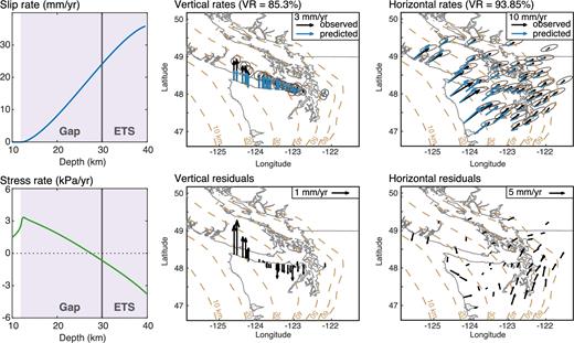
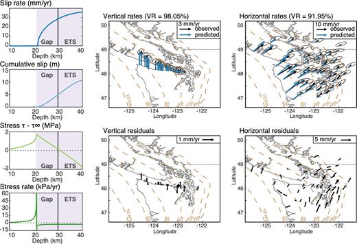
Since the previous model is not sufficient to fit the uplift rates, we consider the derivatives of the coefficients of the Chebyshev polynomials to be non-zero. Consider eq. (10) where |$\dot{a} = 0$| only. We invert here for the locking depth, α, and the Chebyshev coefficients derivatives dc_i/dt. We consider three expansions for the Chebyshev polynomials: N = 2, 4 and 6, where N is the maximum value for the integer i in the polynomial summation. Above N = 6, solutions are too rough to be realistic and would require additional regularization (see Fig. C1 in Appendix C). For N = 6, the best fit is shown in Fig. 7, where the locking depth is 20.48 km of depth and α is −0.31 mm yr⁻¹. This solution is essentially equivalent to the results from Bruhat & Segall (2016) with negative shear stress rates within the shallow slipping zone above the ETS region.

$Best-fitting model from the inversion of interseismic rates in Northern Cascadia using eq. (10), where the deep creeping crack is stationary ($\dot{a}$ = 0), dci/dt ≠ 0 and N = 6. Left: corresponding slip and stress rate profiles. Stress rates are computed by boundary element method. Centre and right: observed and predicted rates. As seen in Bruhat & Segall (2016), deep locking depths, around 20 km, and steep increase in slip rates, corresponding to negative stress rates in the gap and the ETS region, are necessary to fit the uplift rates.$

Figure 7.

Best-fitting model from the inversion of interseismic rates in Northern Cascadia using eq. (10), where the deep creeping crack is stationary (⁠|$\dot{a}$| = 0), dc_i/dt ≠ 0 and N = 6. Left: corresponding slip and stress rate profiles. Stress rates are computed by boundary element method. Centre and right: observed and predicted rates. As seen in Bruhat & Segall (2016), deep locking depths, around 20 km, and steep increase in slip rates, corresponding to negative stress rates in the gap and the ETS region, are necessary to fit the uplift rates.

Open in new tab Download slide

3.4.3 Summary: non-propagating crack models

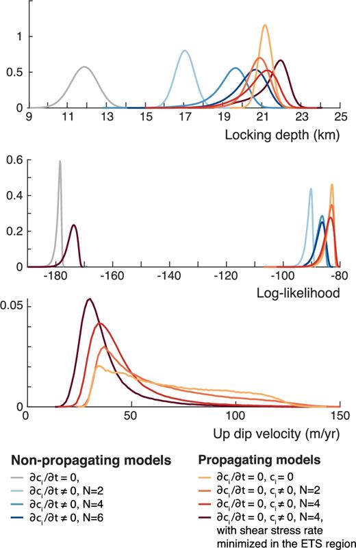
We summarize the results of this subsection in Fig. 8 which displays the marginal distributions of the locking depths, the log-likelihoods and α for the four inversions. The log-likelihood serves as a measure of how well the models fit the observed deformation rates. It is negative and tends towards zero as the fit improves. As mentioned previously, the model where the derivatives of the Chebyshev coefficients dc_i/dt are zero results in shallow locking depth (≈12 km) and large α. However, due to the poor fit to the uplift at coastal stations, the log-likelihood is low. The addition of non-zero dc_i/dt significantly improves the fit. Note that the locking depth increases as more terms are included in the Chebyshev decomposition. The fit to the data improves as well until stabilizing at N = 4 and 6.

Figure 8.

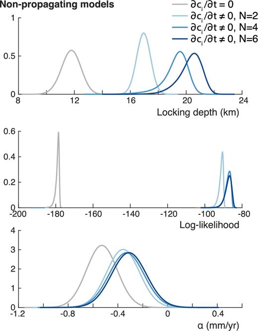
Marginal distributions of the locking depth, the log-likelihood and α for the four inversions of non-propagating models. Note how only models where dc_i/dt ≠ 0 show a significant improvement in fitting the data and deeper looking depths.

Open in new tab Download slide

3.5 Propagating slip

In this section, we allow the creeping region to grow with time, that is, |$\dot{a} \ne 0$|⁠. The slip-rate eq. (10) now includes a propagation term depending on the propagation speed |$\dot{a}$|⁠, t, a and the c_i. Because of the solution non-uniqueness, we explore end-member cases to evaluate how well they explain observed deformation rates in northern Cascadia.

3.5.1 First-order description: c_i = 0 and dc_i/dt = 0 for i > 1

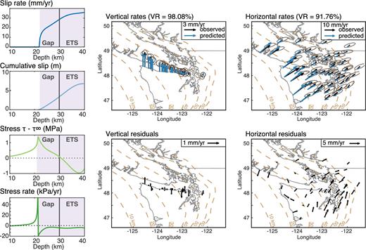
Consider the simplest case where for all i > 1, c_i = 0 and dc_i/dt = 0. This simplification leads to the eqs (13a)–(13d) in the previous section. We invert for the length of the crack a, the propagation velocity |$\dot{a}$|⁠, the loading time t and the reference frame parameter α. The best fit for slip and slip rates are shown in Fig. 9 where the locking depth is 21 km, the propagation speed is 33.4 m yr⁻¹ along the fault, the loading time 296 yr and α = −0.30 mm yr⁻¹. This simple model fits the deformation rates well, in particular the uplift rates. The inferred slip-rate profile is zero above 21 km, then steepens rapidly in the gap and the ETS region. By contrast, the slip profile shows a smooth transition in the same region, leading to a deep slip deficit. The stress profile is linear, maximum and positive at the crack tip, and decreases within the crack. This linear stress change is required to make the stress non-singular at the bottom of the locked region. The stress rates are negative within the crack, reaching −15 kPa yr⁻¹ just behind the crack tip.

Figure 9.

Best-fitting model from the inversion of interseismic rates in Northern Cascadia using eqs (13a)–(13d), where the deep creeping crack migrates updip, and all c_i and dc_i/dt = 0 for i > 1. Left: corresponding slip-rate, cumulative slip, stress and stress rate profiles. Stress and stress rate profiles are computed by boundary element method. Centre and right: observed and predicted rates.

Open in new tab Download slide

3.5.2 dc_i/dt = 0, but c_i ≠ 0

Although the first-order model fits the deformation rates in Cascadia, it corresponds to first-order linear stress changes, as shown in Fig. 2, that are probably too simple to describe the processes acting on the fault. In this section, we add some complexity to the crack model to test different solutions, which could, for instance, optimize expected characteristics of the stress distribution. First consider the case where the coefficients c_i of the Chebyshev polynomials are constant with respect to time, in other words, all derivatives dc_i/dt are zero.

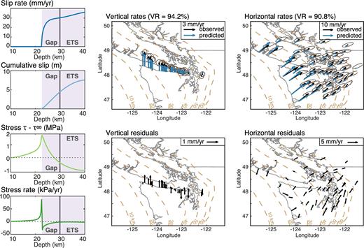
We invert then for the locking depth, α, the propagation velocity |$\dot{a}$|⁠, the loading time t and the c_i. We only consider the expansions for N = 2 and 4, since, as shown in Fig. C2 in Appendix C, solutions are too rough (without additional regularization) to be realistic for higher values of N. For N = 4, the best-fit solution is shown in Fig. 10. As expected, the fault is locked above ∼22 km depth, where the slip rate increases rapidly. Stress rates are negative within the crack, ranging from −20 to −5 kPa yr⁻¹.

Figure 10.

Best-fitting model from the inversion of interseismic rates in Northern Cascadia using eq. (10), where the deep creeping crack migrates updip, and all dc_i/dt = 0. The Chebyshev expansion includes terms up to N = 4. Left: corresponding slip-rate, cumulative slip, stress and stress rate profiles. Stress and stress rate profiles are computed by boundary element method. Centre and right: observed and predicted rates.

Open in new tab Download slide

3.5.3 Propagating slip with minimized stress rates in the ETS region

The negative stress rates observed in the previous inversion are similar to those inferred for the non-propagating crack model. While Bruhat & Segall (2016) found it difficult to explain these rates, the model we propose, where the crack migrates updip, provides a solution without requiring a decrease in fault strength with time at a fixed point.

Forward rate and state-dependent numerical modeling also suggested that the net change in shear stress within the ETS zone is nearly zero; stress accumulates between SSEs, then is fully relaxed during them. We now explore whether inversions can satisfy that constraint by refining the inversion to also minimize shear stress rates in the ETS region.

Inversions for slip rates |$\mathbf {\dot{s}}$| follow the standard approach:

\begin{equation} \mathbf {d} = \mathbf {G} \mathbf {\dot{s}} + \epsilon \quad \textrm{with} \quad \epsilon \sim \mathcal {N}(0,\mathbf {\Sigma }). \end{equation}

(16)

But stress rate also relates to the slip rate through elastic Green's functions, which include the free-surface effects:

\begin{equation} \mathbf {\dot{\tau }} = \mathbf {A} \mathbf {\dot{s}}, \end{equation}

(17)

where the overdot indicates total derivative. We then estimate |$\mathbf {\dot{s}}$| by solving this new regularized least-squares problem which seeks to minimize the stress rate within the ETS zone:

\begin{equation} \textrm{min } || \mathbf {\Sigma }^{-1/2}(\mathbf {G} \mathbf {\dot{s}} - \mathbf {d}) ||^{2}_{2} + \lambda ^{2} || \mathbf {A} \mathbf {\dot{s}}\textrm { (z $\in$ ETS)} ||^{2}_{2} \end{equation}

(18)

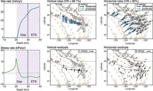
As previously, we invert here for the locking depth, |$\dot{a}$|⁠, t, c_i and α, through an MCMC procedure. λ the regularization parameter is qualitatively chosen to maintain both a good fit within uncertainties and limited shear stress rate in the ETS region. We assume again that the derivatives of the c_i are zero. Solutions that respect the stress rate constraint are found for N ≥ 4. The best fit when N = 4 for slip and stress rates is shown in Fig. 11, in which the locking depth is 21.9 km, the propagation speed 41.3 m yr⁻¹, α = −0.05 mm yr⁻¹ and t = 210 yr. The shapes of the slip and stress distributions are very similar to the best fit obtained in the previous inversion. Stress rates are negative in the gap, while nearly zero as constrained, in the ETS region. Shear stress is maximum at the crack tip, slowly decreases within the crack, reaching a stress drop of 1 MPa at the bottom of the ETS region. In this solution, the gap acts as a ‘cohesive’ region, that is, a region where stress reduces within the crack.

Figure 11.

Best-fitting model from the inversion of interseismic rates in Northern Cascadia using eq. (10), where the crack migrates updip, and all dc_i/dt = 0. The Chebyshev expansion is done up to N = 4 and stress rate is constrained to be zero in the ETS region. Left: corresponding slip-rate, cumulative slip, stress and stress rate profiles. Right: observed and predicted rates.

Open in new tab Download slide

3.5.4 Summary: propagating models where dc_i/dt = 0

The results of the inversions where dc_i/dt = 0, including the first-order expansion, are summarized in Fig. 12. The posterior distribution of the loading time t, the updip velocity |$\dot{a}$|⁠, the locking depth, the log-likelihood and α are displayed for four inversions. First note that the time distribution is very broad and even close to uniform, when c_i ≠ 0 and N = 2. The first-order expansion (c_i = 0) slightly favours models with shorter loading time, whereas the solutions with c_i ≠ 0 and N = 4 prefer loading times closer to 315 yr. Taken literally, this implies that crack propagation would have started right after the last megathrust in Cascadia. The first-order model yields updip velocities ranging rather uniformly from 30 to 120 m yr⁻¹ along the fault, that is, between 4 and 17 m yr⁻¹ in depth (assuming the fault dip is 8°). As more c_i term are added, the velocities decrease to concentrate between 20 and 50 m yr⁻¹ along fault. These are extremely slow velocities, yet still critical to fit the data. Admissible locking depths vary from 19 to 23 km. The unconstrained models fit the data equally well. Due to the regularization, the log-likelihoods of the model where shear stress rates are minimized are, as expected, lower compared to constrained inversions.

Figure 12.

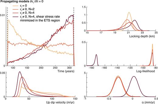
Marginal distributions of the loading time, the updip velocity, the locking depth, the log-likelihood and α for four inversions of propagating models where dc_i/dt = 0.

Open in new tab Download slide

4 DISCUSSION

This work explored various mechanical models to explain the long-term deformation rates observed in Northern Cascadia. The first model, already considered in Bruhat & Segall (2016), assumes that the locking depth is fixed during the interseismic period. To explain the high slip-rate gradients at the base of the locked zone needed to fit the surface data, negative shear rates in the gap and the ETS region are required. Temporal variations in shear stress could be explained either by decreasing the friction coefficient or the effective normal stress acting on the fault. In subduction zones, increasing dehydration reactions, leading to positive pore pressure rate, could cause such temporal changes in effective normal stress. However, it is difficult to understand how the required decrease in frictional resistance could be sustained over long periods of time.

This study shows that slow propagation of interseismic creep into the locked zone could also generate the steep slip-rate gradient, and associated negative shear stress rates, required to fit the geodetic data. Because of the crack propagation, the total stress rate dτ/dt includes the effect of propagation:

\begin{eqnarray} \frac{d\tau (\xi ,t)}{dt} &=& \frac{\partial \tau }{\partial t} + \frac{\partial \tau }{\partial \xi }\frac{\partial \xi }{\partial t}= \frac{\partial \tau }{\partial t} + \frac{\partial \tau }{\partial \xi }\frac{1-\xi }{a}\dot{a}. \end{eqnarray}

(19)

If A is the matrix relating slip s to shear stress τ, then |$\mathbf {\dot{\tau }} = \mathbf {A} \mathbf {\dot{s}}$| as in eq. (17), where overdot indicates total derivative. Recall that because of the influence of the free surface, the total shear stress rate |$\mathbf {\dot{s}}$| is computed using the slip-rate profile through the BEM implementation of A. The propagation term is computed from the spatial gradient of the stress distribution, using the second term in eq. (19). The term ∂τ/∂t can then be computed by subtracting the propagation term from the BEM-derived stress rate. This is illustrated in Fig. 13 which shows slip rates and stress rates (dτ/dt) for the two best-fitting solutions for propagating models from the previous section (presented in Figs 9 and 10). In both cases, the total shear stress rate is dominated by the propagation effect, while the ∂τ/∂t term is considerably smaller in magnitude.

Figure 13.

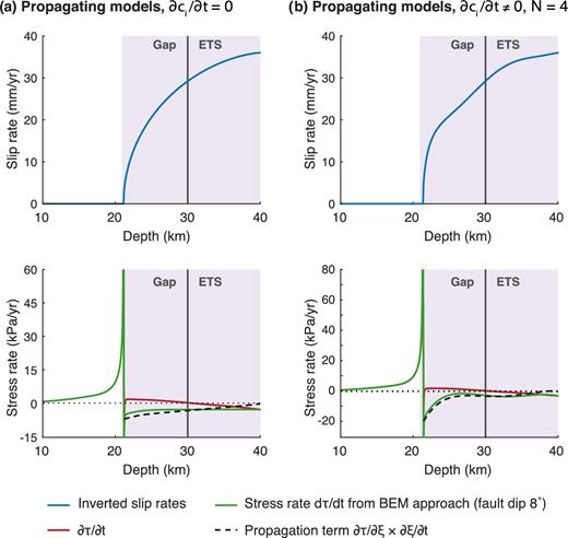
Slip rates and stress rate profiles for two best-fitting solutions for propagating slip distributions. Stress rates do take into account the effect of the free surface (for a 8° dipping fault).

Open in new tab Download slide

The propagating crack provides an alternative solution for the negative shear stress rates, without a temporal decrease in crack stress, and by extension fault strength. Fig. 14 provides a schematic explanation for a crack in which both the peak and residual strength are independent of time. Propagation of the crack to the left results in a decrease in shear stress, for example negative stress rate. Note that this does not require a change in fault strength; the peak-to-residual stress change remains constant, yet produces non-zero shear stress rate.

Figure 14.

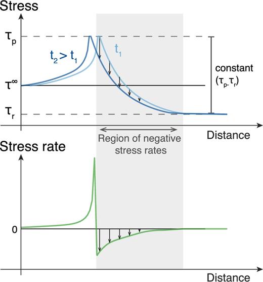
Schematic of how propagation of a crack with constant peak τ_p and residual stress τ_r produces negative shear stress rates. Top: stress profiles at two times. Bottom: resulting stress rate profile.

Open in new tab Download slide

Long-term deformation records can then be described by a very slow updip propagation of the interseismic creep in the gap and the ETS region. As creep penetrates into the updip locked region, the slip-rate profile steepens, producing larger slip rates compared to a static model. The predicted propagation velocities ranges from 30 to 120 m yr⁻¹ along the fault (see Fig. 15). Might this propagation be detected directly in deformation data? Considering that the fault dip is ∼8°, the locking depth migrates at speeds from 4 to 17 m yr⁻¹. Even with 20+ yr of GPS measurements in northern Cascadia, the change of locking depth would reach a maximum 500 m, far less than the uncertainties in the locking depths inferred by kinematic inversions (Burgette et al. 2009). This updip propagation could have been easily missed in long-term observations.

Figure 15.

Summary of marginal distributions of the updip velocity, the locking depth and the log-likelihood for all inversions.

Open in new tab Download slide

Updip propagation of interseismic creep, while very slow, produce accelerations in surface displacements. As the crack propagates updip, both slip-rate and acceleration profiles evolve with time. Consider the first-order approximation described in Section 2, and compute the associated acceleration profile. The time derivative of the slip rate from eq. (13d) is

\begin{eqnarray} \frac{d^2s}{dt^2} = \frac{2v^{\infty }}{a\pi }(1-\xi )\sqrt{1-\xi ^2}\Bigg [2\dot{a} - \frac{\dot{a}^2t}{a}\frac{3\xi +2}{1+\xi } + \ddot{a}t \Bigg ] \end{eqnarray}

(20)

where ä the acceleration of the crack length. The general expression with the Chebyshev expansion is given in Appendix A. Assuming that the propagation speed |$\dot{a}$| does not change with time, that is, |$\ddot{a}=0$|⁠, we can compute the resulting slip and surface accelerations for the best-fitting model displayed in Fig. 9. Fig. 16 shows that slip acceleration evolves from 0 at the bottom of the ETS region to 0.6 mm yr⁻¹² at the crack tip. Synthetic surface accelerations shows that the effect of the updip propagation results in increased uplift at the coastal stations, and decelerating motion in Puget Sound. Now, could we be able to see these accelerations in the surface data? Recent studies, such as Mavrommatis et al. (2015), have reported the existence of decadal-scale transient deformation along the Japan trench. Inferred horizontal accelerations are of the order of 1–1.5 mm yr⁻¹², corresponding up to 3 mm yr⁻¹² on the plate interface, which is 20 times greater than the synthetic accelerations computed here for northern Cascadia. Therefore, we do not expect to observe this updip propagation in surface deformation records for some considerable time.

Figure 16.

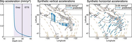
Slip acceleration profile and resulting surface accelerations computed from the best-fitting model presented in Fig. 9.

Open in new tab Download slide

In our model, the time t comes from the boundary condition at the end of the crack, that we set to δ^∞= v^∞t. Within this framework, it corresponds to the length of time that the crack has propagated. Unfortunately, we lack information on the early times of the current interseismic period, and had to assume that t ranges from the maximum age of the deformation data (80 yr) and the time since the last megathrust event. As shown in the inversions, the posterior distributions for the loading time are close to uniform, with a tendency towards values near the upper bound. Except for the first-order description model, solutions favour cracks which started growing in the first half of the interseismic period (t > 200 yr). This suggests that slow propagation would have started soon after the megathrust event, potentially towards the end of the post-seismic period. However, the difficulty is that there might have been post-seismic slip at the crack depth too. In that case, the inferred δ^∞ would be larger than v^∞t, where t is the elapsed time. Thus, it is possible that the inferred time could be less than elapsed time.

The determination of the loading time is however a crucial parameter as it correlates directly with the updip propagation velocity. Fig. 17 displays the correlations between t and |$\dot{a}$| for the two categories of propagating models described in the previous section. The inverse relation between time and speed for the first-order model (c_i and dc_i/dt = 0) is clear considering eq. (13d). One might expect that the addition of the c_i in the propagation term in the general slip-rate expression (eq. 10) changes the correlation. Apart from the spread of the distribution in Fig. 17(b), the overall inverse relationship remains the same.

$Correlation between time t and the updip velocity $\dot{a}$ for two types of inversions.$

Figure 17.

Correlation between time t and the updip velocity |$\dot{a}$| for two types of inversions.

Open in new tab Download slide

The analysis here computes the instantaneous slip rate at a particular time t, yet the available deformation data average over 80 yr for the uplift rates and 15 yr for the GPS data. Thus, the propagation speed, slip-rate and stress-rate distributions must be considered to be averages over a time span of decades. If the propagation was faster, truly time-dependent inversion techniques could be employed to image the space–time evolution of slip (Segall & Matthews 1997; Bartlow et al. 2011).

Changes in effective normal stress with depth could affect the crack propagation speed. In subduction zones where ETS events are observed, effective normal stress is inferred to vary from ∼1 MPa in the ETS region (Audet et al. 2009; Audet & Bürgmann 2014) to at least tens of MPa at seismogenic depths. The mechanical transition between these regions and its length are both unknown. Dehydration reactions are thought to account for higher pore pressure, and lower effective normal stress, within the ETS region. If the crack migrates updip and enters a region of higher effective normal stress region, the rate of propagation should reduce. The corollary to this is that deep interseismic creep might have then propagated faster through the gap and ETS zone in the past, although the available data are insufficient to test this possibility.

The possibility for a migrating locking depth may dramatically change hazard assessment in northern Cascadia. Despite the shrinkage of the locked region due to the updip migration of the locking depth, all inverted models showed that while the slip-rate transition might be abrupt, there could be significant slip deficit below the locking depth. Using such propagating models, slip deficit estimations, which in the conventional framework is solely defined by the slip-rate distribution, have to be reevaluated.

Despite the necessary improvements mentioned above, the proposed model for propagating crack provides a useful tool to detect and characterize possible non-stationary behaviours in surface deformation. It provides a simple method for building non-singular stress and slip profiles, and their time derivatives, of creeping regions. The flexibility offered by the Chebyshev expansion allows the reproduction of stress characteristics observed in numerical simulations, as shown in Fig. 11. It also establishes a first step to bridge purely kinematic inversions to fully physics-based models. Its simplicity allows for inversions of physical characteristics of the fault interface, which are often too computationally expensive when considering quasi-dynamic, or fully dynamic, simulations of earthquake cycles. On the other hand, the proposed model can be used as a guide, or as a first step to more comprehensive numerical simulations.

5 CONCLUSIONS

Most inversions consider the depth distribution of interseismic fault slip rate to be time invariant. In the present work, we develop a new method to characterize interseismic slip rates, that allows slip to penetrate updip into the locked region. Deep interseismic slip is described as a crack with no stress singularity at its tip, loaded at constant slip rate at the downdip end. This model enables us to derive analytical expressions for slip and slip rate, approximately related to shear stress and rate on the fault. We apply this method to describe the long-term deformation rates in northern Cascadia. We first recover the previous result where the crack size is time invariant, and where negative shear stress rates and deep locking depths are needed to fit observed uplift rates. We demonstrate then a new class of solutions, where the locking depth migrates updip with time. Best-fitting models reveal that a very slow updip propagation, between 30 and 120 m yr⁻¹ along the fault is needed to fit the data and that the gap seems to act as a cohesive region where shear strength decreases with slip. The updip propagation provides a plausible explanation for the steep slip-rate profile and the negative shear stress rates inferred in northern Cascadia without requiring temporal changes of the fault strength.

Acknowledgements

This work was supported by the U.S. Geological Survey (G15AP00066). GPS data used in this study are made available by PANGA, the Pacific Northwest Geodetic Array, Central Washington University (http://www.geodesy.cwu.edu/data/bysite) and published in Bruhat & Segall (2016). The leveling and tide gauge data sets are made available in Krogstad et al. (2016). We thank the editor Duncan Agnew, Kaj Johnson and an anonymous reviewer for their insightful comments.

REFERENCES

Atwater

B.F.

,

1987

.

Evidence for great Holocene earthquakes along the outer coast of Washington State

,

Science

236

(

4804

),

942

–

944

.

Audet

P.

,

Bürgmann

R.

,

2014

.

Possible control of subduction zone slow-earthquake periodicity by silica enrichment

,

Nature

509

(

7505

),

389

–

392

.

Audet

P.

,

Bostock

M.G.

,

Christensen

N.I.

,

Peacock

S.M.

,

2009

.

Seismic evidence for overpressured subducted oceanic crust and megathrust fault sealing

,

Nature

457

(

7225

),

76

–

78

.

Avouac

J.-P.

,

Meng

L.

,

Wei

S.

,

Wang

T.

,

Ampuero

J.-P.

,

2015

.

Lower edge of locked Main Himalayan Thrust unzipped by the 2015 Gorkha earthquake

,

Nat. Geosci.

8

(

9

),

708

–

711

.

Bartlow

N.M.

Miyazaki

S.

Bradley

A.M.

Segall

P.

,

2011

.

Space-time correlation of slip and tremor during the 2009 Cascadia slow slip event

,

Geophys. Res. Lett.

38

L18309

,

doi:10.1029/2011GL048714

.

Bilby

B.A.

Eshelby

J.D.

,

1968

.

Dislocations and the theory of fracture

, in

Fracture, An Advanced Treatise

pp.

99

–

182

,

Academic Press

,

New York and London

.

Bruhat

L.

,

Segall

P.

,

2016

.

Coupling on the northern Cascadia subduction zone from geodetic measurements and physics-based models

,

J. geophys. Res.

121

(

11

),

8297

–

8314

.

Burgette

R.J.

Weldon

R.J.

Schmidt

D.A.

,

2009

.

Interseismic uplift rates for western Oregon and along-strike variation in locking on the Cascadia subduction zone

,

J. geophys. Res.

114

B01408

,

doi:10.1029/2008JB005679

.

Dragert

H.

,

Wang

K.

,

Rogers

G.

,

2004

.

Geodetic and seismic signatures of episodic tremor and slip in the northern Cascadia subduction zone

,

Earth Planets Space

56

(

12

),

1143

–

1150

.

Erdogan

F.

,

Gupta

G.D.

,

1972

.

On the numerical solution of singular integral equations

,

Q. Appl. Math.

29

(

4

),

525

–

534

.

Flück

P.

,

Hyndman

R.D.

,

Wang

K.

,

1997

.

Three-dimensional dislocation model for great earthquakes of the Cascadia Subduction Zone

,

J. geophys. Res.

102

(

B9

),

20 539

–

20 550

.

Goldfinger

C.

,

Nelson

C.H.

,

Johnson

J.E.

,

2003

.

Holocene earthquake records from the Cascadia subduction zone and northern San Andreas Fault based on precise dating of offshore turbidites

,

Annu. Rev. Earth planet. Sci.

31

(

1

),

555

–

577

.

Gudmundsson

S.

Sigmundsson

F.

Carstensen

J.M.

,

2002

.

Three-dimensional surface motion maps estimated from combined interferometric synthetic aperture radar and GPS data

,

J. geophys. Res.

107

(

B10

), ETG 13–1–ETG

13

–

14

.

Hearn

E.H.

,

Thatcher

W.R.

,

2015

.

Reconciling viscoelastic models of postseismic and interseismic deformation: effects of viscous shear zones and finite length ruptures

,

J. geophys. Res.

120

(

4

),

2794

–

2819

.

Hills

D.A.

Kelly

P.A.

Dai

D.N.

Korsunsky

A.M.

,

1996

.

Solution of Crack Problems

Solid Mechanics and Its Applications, Vol. 44

,

Springer Netherlands

,

Dordrecht

.

Holtkamp

S.

,

Brudzinski

M.R.

,

2010

.

Determination of slow slip episodes and strain accumulation along the Cascadia margin

,

J. geophys. Res.

115

B00A17

,

doi:10.1029/2008JB006058

.

Hyndman

R.D.

,

2013

.

Downdip landward limit of Cascadia great earthquake rupture

,

J. geophys. Res.

118

(

10

),

5530

–

5549

.

Hyndman

R.D.

,

Wang

K.

,

1995

.

The rupture zone of Cascadia great earthquakes from current deformation and the thermal regime

,

J. geophys. Res.

100

(

B11

),

22 133

–

22 154

.

Ide

S.

,

Baltay

A.

,

Beroza

G.C.

,

2011

.

Shallow dynamic overshoot and energetic deep rupture in the 2011 Mw 9.0 Tohoku-Oki Earthquake

,

Science

332

(

6036

),

1426

–

1429

.

James

T.S.

,

Gowan

E.J.

,

Wada

I.

,

Wang

K.

,

2009

.

Viscosity of the asthenosphere from glacial isostatic adjustment and subduction dynamics at the northern Cascadia subduction zone, British Columbia, Canada

,

J. geophys. Res.

114

B04405

,

doi:10.1029/2008JB006077

.

Jiang

J.

,

Lapusta

N.

,

2016

.

Deeper penetration of large earthquakes on seismically quiescent faults

,

Science

352

(

6291

),

1293

–

1297

.

Johnson

K.M.

Segall

P.

,

2004

.

Viscoelastic earthquake cycle models with deep stress-driven creep along the San Andreas fault system

,

J. geophys. Res.

109

B10403

,

doi:10.1029/2004JB003096

.

Google Scholar

OpenURL Placeholder Text

WorldCat

Krogstad

R.D.

,

Schmidt

D.A.

,

Weldon

R.J.

,

Burgette

R.J.

,

2016

.

Constraints on accumulated strain near the ETS zone along Cascadia

,

Earth planet. Sci. Lett.

439

109

–

116

.

Mavrommatis

A.P.

,

Segall

P.

,

Uchida

N.

,

Johnson

K.M.

,

2015

.

Long-term acceleration of aseismic slip preceding the M w 9 Tohoku-oki earthquake: constraints from repeating earthquakes

,

Geophys. Res. Lett.

42

(

22

),

9717

–

9725

.

McCaffrey

R.

et al. ,

2007

.

Fault locking, block rotation and crustal deformation in the Pacific Northwest

,

Geophys. J. Int.

169

(

3

),

1315

–

1340

.

McCaffrey

R.

,

King

R.W.

,

Payne

S.J.

,

Lancaster

M.

,

2013

.

Active tectonics of northwestern US inferred from GPS-derived surface velocities

,

J. geophys. Res.

118

(

2

),

709

–

723

.

McCrory

P.A.

,

Blair

J.L.

,

Waldhauser

F.

,

Oppenheimer

D.H.

,

2012

.

Juan de Fuca slab geometry and its relation to Wadati-Benioff zone seismicity

,

J. geophys. Res.

117

B09306

,

doi:10.1029/2012JB009407

.

Obara

K.

,

2011

.

Characteristics and interactions between non-volcanic tremor and related slow earthquakes in the Nankai subduction zone, southwest Japan

,

J. Geodyn.

52

(

3–4

),

229

–

248

.

Satake

K.

,

2003

.

Fault slip and seismic moment of the 1700 Cascadia earthquake inferred from Japanese tsunami descriptions

,

J. geophys. Res.

108

(

B11

),

2535

,

doi:10.1029/2003JB002521

.

Satake

K.

,

Shimazaki

K.

,

Tsuji

Y.

,

Ueda

K.

,

1996

.

Time and size of a giant earthquake in Cascadia inferred from Japanese tsunami records of January 1700

,

Nature

379

(

6562

),

246

–

249

.

Savage

J.

,

Burford

R.

,

1970

.

Accumulation of tectonic strain in California

,

Bull. seism. Soc. Am.

60

(

6

),

1877

–

1896

.

Google Scholar

OpenURL Placeholder Text

WorldCat

Segall

P.

,

2010

.

Earthquake and Volcano Deformation

Princeton Univ. Press

.

Segall

P.

,

Bradley

A.M.

,

2012

.

Slow-slip evolves into megathrust earthquakes in 2D numerical simulations

,

Geophys. Res. Lett.

39

L18308

,

doi:10.1029/2012GL052811

.

Segall

P.

,

Matthews

M.

,

1997

.

Time dependent inversion of geodetic data

,

J. geophys. Res.

102

(

B10

),

22 391

–

22 409

.

Takeuchi

C.S.

Fialko

Y.

,

2012

.

Dynamic models of interseismic deformation and stress transfer from plate motion to continental transform faults

,

J. geophys. Res.

117

B05403

,

doi:10.1029/2011JB009056

.

Wech

A.G.

,

Bartlow

N.M.

,

2014

.

Slip rate and tremor genesis in Cascadia

,

Geophys. Res. Lett.

41

(

2

),

392

–

398

.

Wech

A.G.

,

Creager

K.C.

,

2011

.

A continuum of stress, strength and slip in the Cascadia subduction zone

,

Nat. Geosci.

4

(

9

),

624

–

628

.

Wech

A.G.

,

Creager

K.C.

,

Melbourne

T.I.

,

2009

.

Seismic and geodetic constraints on Cascadia slow slip

,

J. geophys. Res.

114

B10316

,

doi:10.1029/2008JB006090

.

APPENDIX A: SLIP AND SLIP-RATE POLYNOMIAL DECOMPOSITIONS FOR A CRACK DRIVEN BY A DISLOCATION WITH A NON-SINGULAR STRESS DISTRIBUTION AT THE CRACK TIP IN A FULL SPACE

A1 Burgers vector distribution

Consider a 1-D crack of length a in a full space loaded at constant long-term rate v^∞ at depth (Fig. 1). The medium is loaded at spatially uniform stress τ^∞. The stress acting on the fault is τ, such that the stress drop is defined as Δτ = τ^∞ − τ. The goal is to derive a general expression for slip and slip rate for which stress is non-singular. This condition, equivalent to negating the stress intensity factor K, is given by Bilby & Eshelby (1968):

\begin{eqnarray} \nonumber \int _{-1}^{1} \frac{\Delta \tau (u) }{\sqrt{1-u^2}}du&=& 0, \\ \int _{-1}^{1} \frac{u \Delta \tau (u) }{\sqrt{1-u^2}}du &=& 0. \end{eqnarray}

(A1)

where distance is normalized by the full crack length a, (ξ = z/a). Using eq. (4.7) from Segall (2010, chap. 4), which follows Bilby & Eshelby (1968),

\begin{equation} B(\xi ) = -\frac{2}{\mu ^{*} \pi }\int _{-1}^{1} \frac{\Delta \tau (u) \sqrt{1-u^2}}{(\xi -u)\sqrt{1-\xi ^2}} du+ \frac{2 A}{a\sqrt{1-\xi ^2}} , \end{equation}

(A2)

where A is a constant proportional to the net dislocation,

\begin{equation} A = \frac{1}{\pi }\int _{-1}^{1} B(u) du. \end{equation}

(A3)

If the crack is in-plane shear (mode II), μ* = μ/(1 − ν) where μ the shear modulus and ν Poisson's ratio, whereas if the crack is anti-plane (mode III) μ* = μ.

Consider the left-hand term of eq. (A2). Using the identity

\begin{equation} \frac{\sqrt{1-u^2}}{\sqrt{1-\xi ^2}} = \frac{\xi ^2 - u^2}{\sqrt{1-u^2}\sqrt{1-\xi ^2}} + \frac{\sqrt{1-\xi ^2}}{\sqrt{1-u^2}}, \end{equation}

(A4)

we rewrite eq. (A2) as:

\begin{eqnarray} \nonumber B(\xi ) &=& -\frac{2\xi }{\mu ^{*} \pi \sqrt{1-\xi ^2}}\int _{-1}^{1} \frac{\Delta \tau (u) }{\sqrt{1-u^2}}du -\frac{2}{\mu ^{*} \pi \sqrt{1-\xi ^2}}\int _{-1}^{1} \frac{\Delta \tau (u) u}{\sqrt{1-u^2}}du \\ && - \frac{2\sqrt{1-\xi ^2}}{\mu ^{*} \pi }\int _{-1}^{1} \frac{\Delta \tau (u) }{(\xi -u)\sqrt{1-u^2}}du + 2\frac{A}{a\sqrt{1-\xi ^2}}. \end{eqnarray}

(A5)

Now consider the decomposition of the stress drop in the crack in Chebyshev polynomials of the first kind T_i:

\begin{equation} \Delta \tau (u) = \mu ^{*}\sum _{i=0}^{\infty } c_i T_i(u), \end{equation}

(A6)

that satisfy the orthogonality relations

\begin{eqnarray} \int _{-1}^{1}\frac{T_{n}(u)T_{m}(u)}{\sqrt{1-u^{2}}}du={\left\lbrace \begin{array}{@{}l@{\quad }l@{}}\pi \delta _{nm}&n=0\\ {\frac{\pi }{2}\delta _{nm}}&n\ge 1. \end{array}\right.} \end{eqnarray}

(A7)

Note that T₀(u) = 1, T₁(u) = u, and substitute eq. (A6) into eq. (A5)

\begin{eqnarray} \nonumber B(\xi ) &=& -\frac{2\xi }{ \pi \sqrt{1-\xi ^2}}\sum _{i=0}^{\infty }c_i\int _{-1}^{1} \frac{T_i(u) T_0}{\sqrt{1-u^2}}du -\frac{2}{ \pi \sqrt{1-\xi ^2}}\sum _{i=0}^{\infty }c_i\int _{-1}^{1} \frac{T_i(u) T_1}{\sqrt{1-u^2}}du +\frac{2A}{a\sqrt{1-\xi ^2}} \\ && - \frac{2\sqrt{1-\xi ^2}}{ \pi }\sum _{i=0}^{\infty }c_i\int _{-1}^{1} \frac{T_i(u) }{(\xi -u)\sqrt{1-u^2}}du. \end{eqnarray}

(A8)

Our goal is to derive expressions for stress drop such that the conditions given in eq. (A1) are satisfied. The first two terms correspond to non-zero stress intensity that we must eliminate. Given the orthogonality relationship for Chebyshev polynomials, the first term vanishes only when c₀ = 0. Likewise, we find c₁ such that the second term cancels the net dislocation term:

\begin{eqnarray} c_1 = \frac{2 A}{a}. \end{eqnarray}

(A9)

We solve the last integral by using the integral relations between Chebyshev polynomials of the first and second kinds, U_i(ξ)

\begin{equation} \int _{-1}^{1} \frac{ T_i(u) }{(u-\xi )\sqrt{1-u^2}} du = - \pi U_{i-1}(\xi ) \qquad i \ge 1. \end{equation}

(A10)

We can then express B(ξ) as a function of Chebyshev polynomials of the second kind:

\begin{eqnarray} B(\xi ) &=& 2\sqrt{1-\xi ^2} c_1 U_0+2\sqrt{1-\xi ^2}\sum _{i=2}^{\infty } c_i U_{i-1}(\xi ). \end{eqnarray}

(A11)

Given c₁ = 2A/a and U₀ = 1, the expression of the Burgers vector distribution is:

\begin{eqnarray} B(\xi ) &=& \frac{4 A}{a}\sqrt{1-\xi ^2}+2\sqrt{1-\xi ^2}\sum _{i=2}^{\infty } c_i U_{i-1}(\xi ) . \end{eqnarray}

(A12)

A2 Slip distribution

We first construct a linear mapping such that the downdip limit of the crack stays fixed as the crack grows. Consider the variables ξ and z such that ξ ∈ [−1, 1] and z ∈ [0, a]. The linear mapping between the two variables is:

\begin{eqnarray} \xi &=& 1-\frac{2z}{a}. \end{eqnarray}

(A13)

Slip is integral of dislocation distribution:

\begin{eqnarray} \nonumber s(\xi ) &=& \frac{a}{2}\int _{-1}^{\xi }B(x)dx\\ &=& 2A\int _{-1}^{\xi }\sqrt{1-x^2}dx+a\sum _{i=2}^{\infty }c_i\int _{-1}^{\xi } \sqrt{1-x^2} U_{i-1}(x)dx. \end{eqnarray}

(A14)

Consider the first integral I₁:

\begin{eqnarray} I_1 = \int _{-1}^{\xi }\sqrt{1-x^2}dx = \frac{1}{2} \left[ \xi \sqrt{1-\xi ^2} + \arcsin \xi + \frac{\pi }{2} \right]. \end{eqnarray}

(A15)

For the second integral, change variable x = cos θ

\begin{eqnarray} \nonumber I_2 &=& - \int _{\pi }^{\arccos {\xi }} \sqrt{1-\cos ^2\theta } U_{i-1}(\cos \theta )\sin \theta d\theta \\ &=& - \int _{\pi }^{\arccos {\xi }} \sin ^2\theta U_{i-1}(\cos \theta )d\theta . \end{eqnarray}

(A16)

The Chebyshev polynomials of the second kind satisfy:

\begin{eqnarray} U_i(\cos \theta ) = \frac{\sin ((i+1)\theta )}{\sin \theta }. \end{eqnarray}

(A17)

Thus,

\begin{eqnarray} I_2 &=& -\int _{\pi }^{\arccos {\xi }} \sin \theta \sin (i\theta )d\theta . \end{eqnarray}

(A18)

The integrand can be expanded using sin u sin v = [cos (u − v) − cos (u + v)]/2:

\begin{eqnarray} \nonumber I_2 &=& -\int _{\pi }^{\arccos \xi } \frac{1}{2}[\cos ((i-1)\theta )-\cos ((i+1)\theta )]d\theta \\ &=& -\frac{\sin \big ((i-1)\arccos \xi \big )}{2(i-1)} +\frac{\sin \big ((i+1)\arccos \xi \big )}{2(i+1)}. \end{eqnarray}

(A19)

Since |$\theta = \arccos \xi$|⁠, and making use of eq. (A17)

\begin{eqnarray} \sin \big ((i+1)\theta \big ) = \sin (\theta ) U_{i}(\cos \theta ) &= \sin (\arccos (\xi )) U_{i}(\xi ) &= \sqrt{1-\xi ^2}U_i(\xi ). \end{eqnarray}

(A20)

Likewise,

\begin{eqnarray} \sin \big ((i-1)\theta \big ) = \sin (\theta ) U_{i-2}(\cos \theta ) &= \sin (\arccos (\xi )) U_{i-2}(\xi ) &= \sqrt{1-\xi ^2}U_{i-2}(\xi ). \end{eqnarray}

(A21)

The second integral in the slip expression is then given by:

\begin{eqnarray} I_2 &=& \frac{1}{2}\sqrt{1-\xi ^2}\Bigg [\frac{U_{i}(\xi )}{i+1} -\frac{U_{i-2}(\xi )}{i-1}\Bigg ]. \end{eqnarray}

(A22)

Substituting eqs (A15) and (A22) into eq. (A14) gives:

\begin{eqnarray} s(\xi ) = A\Bigg [\xi \sqrt{1-\xi ^2} + \arcsin \xi + \frac{\pi }{2}\Bigg ]+\frac{a}{2}\sqrt{1-\xi ^2}\sum _{i=2}^{\infty }c_i\Bigg [\frac{U_{i}(\xi )}{i+1} -\frac{U_{i-2}(\xi )}{i-1}\Bigg ]. \end{eqnarray}

(A23)

Using the boundary condition s(ξ = 1) = v^∞t, we compute the dislocation term A:

\begin{eqnarray} A&=& \frac{v^{\infty }t}{\pi }. \end{eqnarray}

(A24)

Thus, the expression of the slip distribution s(ξ) is:

\begin{equation} s(\xi )= \frac{v^{\infty }t}{\pi }\Bigg [\xi \sqrt{1-\xi ^2} + \arcsin (\xi ) + \frac{\pi }{2}\Bigg ]+\frac{a}{2}\sqrt{1-\xi ^2}\sum _{i=2}^{\infty }c_i\Bigg [\frac{U_{i}(\xi )}{i+1} -\frac{U_{i-2}(\xi )}{i-1}\Bigg ]. \end{equation}

(A25)

Given A, we can write B(ξ) [using eq. (A12)]:

\begin{eqnarray} B(\xi ) &=&\frac{4 v^{\infty }t}{a\pi }\sqrt{1-\xi ^2}+2\sqrt{1-\xi ^2}\sum _{i=2}^{\infty } c_i U_{i-1}(\xi ) \end{eqnarray}

(A26)

A3 Slip-rate distribution

Given the slip distribution, we can also derive the slip-rate distribution in term of Chebyshev polynomials. Here, we compute the general case where a and the c_i are functions of time.

A3.1 Total derivative of slip

Using eq. (A13), we compute the time derivative of the spatial variable ξ:

\begin{eqnarray} \frac{\partial \xi }{\partial t} &=& \frac{\partial \xi }{\partial a}\frac{\partial a}{\partial t} = \frac{2z}{a^2}\dot{a} =\frac{1-\xi }{a}\dot{a}. \end{eqnarray}

(A27)

The total time derivative of slip is thus:

\begin{eqnarray} \frac{ds}{dt} &=& \frac{\partial s }{\partial t} +\frac{\partial s }{\partial \xi }\frac{\partial \xi }{\partial t} = \frac{\partial s}{\partial t} + \dot{a}\frac{1-\xi }{a}\frac{\partial s}{\partial \xi }. \end{eqnarray}

(A28)

A3.2 Partial derivative of slip with respect to t

To compute ∂s/∂t, first rewrite s(ξ, t):

\begin{eqnarray} s(\xi ,t) &=& v^{\infty }tg(\xi ) + \frac{a(t)}{2}\sum _{i=2}^{\infty }c_i f_{i}(\xi ), \end{eqnarray}

(A29)

where the functions g and f_i are defined as:

\begin{eqnarray} g(\xi ) &=& \frac{1}{\pi }\Bigg [\xi \sqrt{1-\xi ^2} + \arcsin \xi + \frac{\pi }{2}\Bigg ], \end{eqnarray}

(A30)

\begin{eqnarray} f_i(\xi ) &=& \sqrt{1-\xi ^2}\Bigg [\frac{U_{i}(\xi )}{i+1} -\frac{U_{i-2}(\xi )}{i-1}\Bigg ]. \end{eqnarray}

(A31)

Thus,

\begin{eqnarray} \frac{\partial s}{\partial t} &=& v^{\infty }g(\xi ) + \frac{a}{2} \sum _{i=2}^{\infty }\frac{d c_i}{d t} f_{i}(\xi )+ \frac{\dot{a}}{2} \sum _{i=2}^{\infty }c_i f_{i}(\xi ). \end{eqnarray}

(A32)

Combine eqs (A28) and (A32):

\begin{eqnarray} \frac{ds}{dt} &=& v^{\infty }g(\xi )+ \frac{a}{2} \sum _{i=2}^{\infty }\frac{d c_i}{dt} f_{i}(\xi ) + \dot{a}\Bigg [\frac{d g}{d \xi }\frac{1-\xi }{a}v^{\infty }t+ \frac{1}{2}\sum _{i=2}^{\infty }c_i \Bigg (f_{i}(\xi ) + \frac{d f_i(\xi )}{d \xi }(1-\xi )\Bigg )\Bigg ]. \end{eqnarray}

(A33)

The derivative of g and f_i with respect to ξ are:

\begin{eqnarray} \frac{d g}{d \xi } &=& g^{\prime } = \frac{2}{\pi }\sqrt{1-\xi ^2}, \end{eqnarray}

(A34)

\begin{eqnarray} \frac{d f_i}{d \xi } &=& f_i^{\prime } = 2\sqrt{1-\xi ^2}U_{i-1}. \end{eqnarray}

(A35)

The last relation follows from eq. (A22).

A4 Stress drop within the crack and stress drop rate

Consider the decomposition of the stress drop in the crack in Chebyshev polynomials. We have shown that c₀ = 0 and c₁ = 2v^∞t/aπ. As a result, eq. (A6) becomes:

\begin{equation} \Delta \tau (\xi ) = \mu ^{*}\frac{ 2v^{\infty } t}{\pi a}\xi + \mu ^{*} \sum _{i=2}^{\infty } c_i T_i(\xi ). \end{equation}

(A36)

The total stress drop rate within the crack is thus:

\begin{eqnarray} \frac{d\Delta \tau (\xi ,t)}{dt} &=& \frac{\partial \Delta \tau }{\partial t} + \frac{\partial \Delta \tau }{\partial \xi }\frac{\partial \xi }{\partial t} = \frac{\partial \Delta \tau }{\partial t} + \frac{\partial \Delta \tau }{\partial \xi }\frac{1-\xi }{a}\dot{a}, \end{eqnarray}

(A37)

where

\begin{eqnarray} \nonumber \frac{\partial \Delta \tau }{\partial t} &=&\frac{2\mu ^{*} v^{\infty }}{\pi a}\xi - \dot{a}\frac{2\mu ^{*} v^{\infty } t}{\pi a^2}\xi + \mu ^{*} \sum _{i=2}^{\infty } \frac{d c_i}{dt} T_i(\xi )\\ \frac{\partial \Delta \tau }{\partial \xi } &=&\frac{2\mu ^{*} v^{\infty }t}{\pi a}+ \mu ^{*} \sum _{i=2}^{\infty } c_i\frac{d T_i(\xi )}{d \xi } = \frac{2\mu ^{*} v^{\infty }t}{\pi a}+ \mu ^{*} \sum _{i=2}^{\infty } c_i iU_{i-1}, \end{eqnarray}

(A38)

making use of the properties of the derivatives of the Chebyshev polynomials:

\begin{eqnarray} \frac{d T_i(\xi )}{d \xi } &=& iU_{i-1}. \end{eqnarray}

(A39)

By substituting eqs (A38) into (A37), we get:

\begin{eqnarray} \frac{d\Delta \tau }{dt} &=& \frac{2\mu ^{*} v^{\infty }}{\pi a}\xi + \mu ^{*} \sum _{i=2}^{\infty } \frac{d c_i}{dt} T_i(\xi )+ \mu ^{*}\frac{\dot{a}}{a}\Bigg (\frac{ 2v^{\infty }t}{\pi a}(1-2\xi )+ (1-\xi )\sum _{i=2}^{\infty } c_i iU_{i-1}\Bigg ). \end{eqnarray}

(A40)

Note that since Δτ = τ^∞ − τ, that dτ/dt = −dΔτ/dt.

A5 Slip acceleration

Here, we use the slip-rate expression (eq. A33) to derive the slip acceleration. We compute the time derivatives of each term. First term:

\begin{eqnarray} \frac{d}{dt}\big (v^{\infty }g\big ) &=& v^{\infty }\frac{\partial g}{\partial t} = v^{\infty }g^{\prime }\frac{1-\xi }{a}\dot{a}. \end{eqnarray}

(A41)

Second term:

\begin{eqnarray} \frac{d}{dt}\Bigg (\frac{a}{2} \sum _{i=2}^{\infty }\frac{d c_i}{dt} f_{i}\Bigg ) &=& \frac{a}{2} \sum _{i=2}^{\infty }\frac{d^2 c_i}{d t^2} f_{i}+ \frac{\dot{a}}{2} \sum _{i=2}^{\infty }\frac{d c_i}{dt}( f_{i} + (1-\xi )f^{\prime }_i ). \end{eqnarray}

(A42)

Third term:

\begin{eqnarray} \frac{d}{dt}\Bigg (\dot{a}g^{\prime }\frac{1-\xi }{a}v^{\infty }t\Bigg ) &=& \ddot{a}g^{\prime }\frac{1-\xi }{a}v^{\infty }t + \frac{\dot{a}}{a}\frac{\partial \big ( (1-\xi )g^{\prime }\big )}{\partial t}v^{\infty }t - \dot{a}^2 g^{\prime }\frac{1-\xi }{a^2}v^{\infty }t + \dot{a}g^{\prime }\frac{1-\xi }{a}v^{\infty }, \end{eqnarray}

(A43)

with

\begin{eqnarray} \frac{\partial (1-\xi )g^{\prime }}{\partial t} &=& \dot{a}\frac{1-\xi }{a}\frac{\partial \big ( (1-\xi )g^{\prime }\big )}{\partial \xi }= \dot{a}\frac{1-\xi }{a}((1-\xi )g^{\prime \prime }-g^{\prime } ). \end{eqnarray}

(A44)

Last term:

\begin{eqnarray} \nonumber \frac{d}{dt}\Bigg (\frac{\dot{a}}{2}\sum _{i=2}^{\infty }c_i \Big (f_{i} + f_i^{\prime }(1-\xi )\Big )\Bigg ) &=& \frac{\ddot{a}}{2}\sum _{i=2}^{\infty }c_i \Big (f_{i} + f_i^{\prime }(1-\xi )\Big ) + \frac{\dot{a}}{2}\sum _{i=2}^{\infty }\frac{d c_i}{dt} (f_{i} + f_i^{\prime }(1-\xi ))\\ && + \frac{\dot{a}}{2}\sum _{i=2}^{\infty } c_i \frac{\partial (f_{i} + f_i^{\prime }(1-\xi ))}{\partial t}, \end{eqnarray}

(A45)

where

\begin{eqnarray} \frac{\partial (f_{i} + f_i^{\prime }(1-\xi ))}{\partial t} &=& \dot{a}\frac{1-\xi }{a} \frac{\partial (f_{i} + f_i^{\prime }(1-\xi ))}{\partial \xi } = \dot{a}\frac{(1-\xi )^2}{a} f_i^{\prime \prime }. \end{eqnarray}

(A46)

By combining eqs (A41), (A42), (A43) and (A45), we get:

\begin{eqnarray} \nonumber \frac{d^2s}{dt^2} &=& \frac{a}{2} \sum _{i=2}^{\infty }\frac{d^2 c_i}{d t^2} f_{i} + \dot{a}\Bigg [\frac{2(1-\xi )}{a}g^{\prime }v^{\infty } + \sum _{i=2}^{\infty }\frac{d c_i}{dt}( f_{i} + (1-\xi )f^{\prime }_i) \Bigg ]\\ \nonumber && + \,\dot{a}^2\Bigg [\frac{v^{\infty }t}{a^2}(1-\xi ) ((1-\xi )g^{\prime \prime }-2g^{\prime } ) + \frac{(1-\xi )}{2a}\sum _{i=2}^{\infty } c_i f_i^{\prime \prime }\Bigg ] \\ && +\, \ddot{a}\Bigg [ g^{\prime }\frac{1-\xi }{a}v^{\infty }t + \frac{1}{2}\sum _{i=2}^{\infty }c_i (f_{i} + f_i^{\prime }(1-\xi ) ) \Bigg ]. \end{eqnarray}

(A47)

APPENDIX B: SPATIAL CORRELATIONS

In this study, we empirically estimate the correlations in the velocities to populate the full covariance matrices. We first compute the variogram (inverse related to the covariance) estimated from the residual velocities. Residuals are derived from the best-fitting inversion for shear stress rates in Bruhat & Segall (2016). The experimental variogram is then plotted against the separation distance between stations, also called the ‘lag’ distance h, and fitted with an exponential variogram model:

\begin{equation} \gamma (h) = b\bigg (1-\exp \bigg (-\frac{h}{h_c}\bigg )\bigg ) \end{equation}

(B1)

where h_c the characteristic distance at which the experimental variogram levels off. Finally, the covariance matrix Σ is constructed using the variance of the residuals r and the characteristic distance h_c:

\begin{equation} \Sigma _{ij} = \mbox{Var}(\mathbf {r})\exp \bigg (-\frac{d_{j}^{i}}{h_c}\bigg ) \end{equation}

(B2)

with |$d_{j}^{i}$| the distance between the stations i and j. Since this method also calculates the variances, if those are smaller than the formal variances of the geodetic measurements, we replace them with the original formal variances. We compute Σ in an iterative manner. We start with a diagonal covariance matrix filled with the formal variances. Using the procedure described above, we compute and update the covariance matrix Σ, then the residuals, until convergence. The estimated h_c is 96.7 km for the GPS east component, 291.1 km for the GPS north component and 3.2 km for the uplift rates obtained from tide gauges and leveling surveys (Fig. B1). The large correlation lengths in the horizontal GPS measurements, compared to that for the uplift rates, decreases the weight of the GPS data in the inversions.

Figure B1.

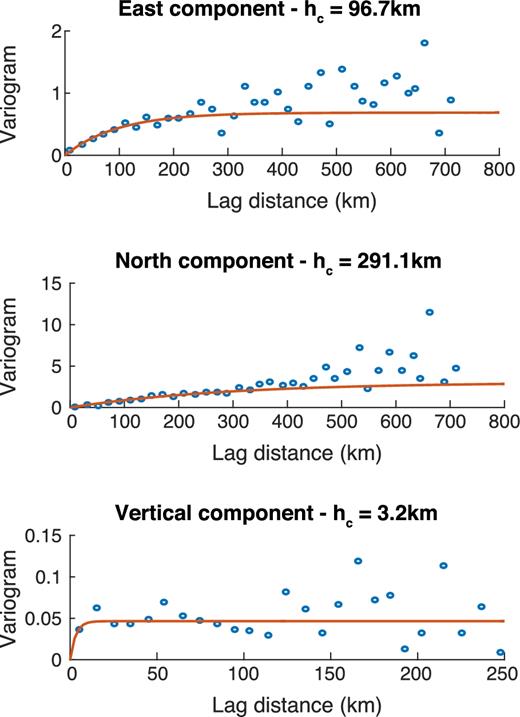
Experimental variograms (blue circles) and fits to an exponential variogram model (red lines) computed from the residuals to the best-fitting shear stress rate inversion from Bruhat & Segall (2016). Large spatial correlations are observed in the horizontal residuals, especially in the north–south component. In contrast, the vertical residuals show close to no spatial correlation.

Open in new tab Download slide

APPENDIX C: INVERSION

In this study, we derive expressions for slip, slip rate, stress and stress rate in the crack as a combination of Chebyshev polynomials. Each expression includes then summations of Chebyshev polynomials for i from i = 2 up to N. As a result, we have to decide on a value for N, that will determine the highest degree in the Chebyshev expansion. In practice, N is found such that the inferred distributions for slip, slip rate, stress and stress rate in the crack are not too rough. Rough solutions are characterized by a significant increase in log-likelihood, that is, a better fit, but unrealistic physical solutions. For the cases where we had to make this choice, Figs C1 and C2 display each the best-fitting models for the chosen N, and for a rougher solution (larger N).

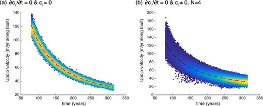
$Best-fitting models for N = 6 and 8 from the inversion of interseismic rates in Northern Cascadia using eq. (10), where the deep creeping crack is stationary ($\dot{a}$ = 0) and dci/dt ≠ 0. (a) Corresponding slip-rate profiles. (b) Posterior distributions for locking depth, log-likelihood and α.$

Figure C1.

Best-fitting models for N = 6 and 8 from the inversion of interseismic rates in Northern Cascadia using eq. (10), where the deep creeping crack is stationary (⁠|$\dot{a}$| = 0) and dc_i/dt ≠ 0. (a) Corresponding slip-rate profiles. (b) Posterior distributions for locking depth, log-likelihood and α.

Open in new tab Download slide

Figure C2.

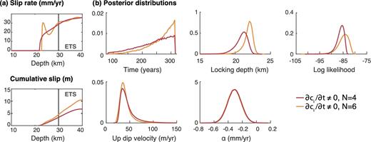
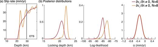
Best-fitting models for N = 4 and 6 from the inversion of interseismic rates in Northern Cascadia using eq. (10), where the deep creeping crack migrates updip, c_i ≠ 0 and all dc_i/dt = 0. (a) Corresponding slip-rate and slip profiles. (b) Posterior distributions for time, locking depth, log-likelihood, updip velocity and α.

Open in new tab Download slide

Download all slides

Month:	Total Views:
July 2017	80
August 2017	138
September 2017	31
October 2017	37
November 2017	109
December 2017	53
January 2018	56
February 2018	57
March 2018	81
April 2018	42
May 2018	66
June 2018	22
July 2018	23
August 2018	37
September 2018	49
October 2018	55
November 2018	36
December 2018	31
January 2019	33
February 2019	43
March 2019	35
April 2019	39
May 2019	47
June 2019	62
July 2019	33
August 2019	23
September 2019	23
October 2019	25
November 2019	29
December 2019	18
January 2020	15
February 2020	17
March 2020	16
April 2020	7
May 2020	9
June 2020	18
July 2020	17
August 2020	7
September 2020	9
October 2020	13
November 2020	12
December 2020	23
January 2021	15
February 2021	10
March 2021	39
April 2021	21
May 2021	12
June 2021	16
July 2021	19
August 2021	18
September 2021	17
October 2021	15
November 2021	13
December 2021	11
January 2022	23
February 2022	14
March 2022	19
April 2022	20
May 2022	11
June 2022	16
July 2022	18
August 2022	20
September 2022	19
October 2022	28
November 2022	16
December 2022	8
January 2023	21
February 2023	20
March 2023	18
April 2023	19
May 2023	13
June 2023	17
July 2023	9
August 2023	7
September 2023	11
October 2023	13
November 2023	11
December 2023	11
January 2024	10
February 2024	29
March 2024	22
April 2024	18
May 2024	25
June 2024	13
July 2024	30
August 2024	7
September 2024	21
October 2024	16
November 2024	25
December 2024	28
January 2025	24
February 2025	18
March 2025	29
April 2025	30

Article Contents

Deformation rates in northern Cascadia consistent with slow updip propagation of deep interseismic creep

Abstract

1 INTRODUCTION

2 METHODS

2.1 Crack models for penetrating creep

2.2 First-order description

3 APPLICATION TO NORTHERN CASCADIA

3.1 Deformation rates

3.2 Slip-rate inversions

3.3 Free-surface effects

3.4 Non-propagating crack

3.4.1 |$\dot{a} = 0$| and dci/dt = 0

3.4.2 |$\dot{a} = 0$| and dci/dt ≠ 0

3.4.3 Summary: non-propagating crack models

3.5 Propagating slip

3.5.1 First-order description: ci = 0 and dci/dt = 0 for i > 1

3.5.2 dci/dt = 0, but ci ≠ 0

3.5.3 Propagating slip with minimized stress rates in the ETS region

3.5.4 Summary: propagating models where dci/dt = 0

4 DISCUSSION

5 CONCLUSIONS

Acknowledgements

REFERENCES

APPENDIX A: SLIP AND SLIP-RATE POLYNOMIAL DECOMPOSITIONS FOR A CRACK DRIVEN BY A DISLOCATION WITH A NON-SINGULAR STRESS DISTRIBUTION AT THE CRACK TIP IN A FULL SPACE

A1 Burgers vector distribution

A2 Slip distribution

A3 Slip-rate distribution

A3.1 Total derivative of slip

A3.2 Partial derivative of slip with respect to t

A4 Stress drop within the crack and stress drop rate

A5 Slip acceleration

APPENDIX B: SPATIAL CORRELATIONS

APPENDIX C: INVERSION

Citations

Views

Altmetric

Email alerts

Astrophysics Data System

Citing articles via

Latest

Most Read

Most Cited

This Feature Is Available To Subscribers Only

3.4.1 |$\dot{a} = 0$| and dc_i/dt = 0

3.4.2 |$\dot{a} = 0$| and dc_i/dt ≠ 0

3.5.1 First-order description: c_i = 0 and dc_i/dt = 0 for i > 1

3.5.2 dc_i/dt = 0, but c_i ≠ 0

3.5.4 Summary: propagating models where dc_i/dt = 0