


Summary
Ambient noise tomography exploits seismic ground motions that propagate coherently over long interstation distances. Such ground motions provide information about the medium of propagation that is recoverable from interstation cross-correlations. Local noise sources, which are particularly strong in ocean bottom environments, corrupt ambient noise cross-correlations and compromise the effectiveness of ambient noise tomography. Based on 62 ocean bottom seismometers (OBSs) located on Juan de Fuca (JdF) plate from the Cascadia Initiative experiment and 40 continental stations near the coast of the western United States obtained in 2011 and 2012, we attempt to reduce the effects of local noise on vertical component seismic records across the plate and onto US continent. The goal is to provide better interstation cross-correlations for use in ambient noise tomography and the study of ambient noise directionality. As shown in previous studies, tilt and compliance noise are major sources of noise that contaminate the vertical channels of the OBSs and such noise can be greatly reduced by exploiting information on the horizontal components and the differential pressure gauge records, respectively. We find that ambient noise cross-correlations involving OBSs are of significantly higher signal-to-noise ratio at periods greater than 10 s after reducing these types of noise, particularly in shallow water environments where tilt and compliance noise are especially strong. The reduction of tilt and compliance noise promises to improve the accuracy and spatial extent of ambient noise tomography, allowing measurements based on coherently propagating ambient noise to be made at stations in the shallower parts of the JdF plate and at longer periods than in previous studies. In addition such local noise reduction produces better estimates of the azimuthal content of ambient noise.
1 INTRODUCTION
One of the major limitations of seismic data recorded by ocean bottom seismometers (OBSs), compared to the land-based stations, is their higher level of locally generated noise. The source of such noise has been well studied over the past few decades (e.g. Webb 1988; Duennebier & Sutton 1995). Two types of noise are believed to be the major source of local noise contamination observed on OBSs: tilt noise, produced by seafloor currents changing the level of poorly situated seismometers, and compliance noise, produced by pressure variations induced by ocean gravity waves that deform the solid earth below the seismometer. Crawford & Webb (2000) and Webb & Crawford (1999) showed that both types of noise may be greatly reduced by predicting/subtracting the noise component derived, respectively, from the horizontal components of the seismometer for the tilt noise and from the differential pressure gauge (DPG) for the compliance noise. These techniques have been applied successfully to earthquake data to improve the signal-to-noise ratio (SNR) and to reduce distortions (e.g. Dolenc et al.2007; Ball et al.2014). Bell et al. (2015) investigated the characteristics of both tilt and compliance noise recorded on the Cascadia Initiative stations across the Juan de Fuca (JdF) plate and showed that local noise on the vertical components can be reduced by one to two orders of magnitude by removing these types of noise.
In recent studies, ambient noise tomography (ANT) has proven to be effective at constraining the crust and upper mantle structure based on cross-correlations of long time sequences of ambient noise. The method seeks to exploit ambient noise that is generated far from the two stations whose seismic records are cross-correlated and propagates coherently between the stations. Fairly standard methods have been developed for continental stations to process raw seismic data for this purpose (e.g. Bensen et al.2007). In an oceanic environment, near mid-ocean ridges, Harmon et al. (2007) and Yao et al. (2011) showed that the fundamental and first higher mode Rayleigh waves can be extracted from ambient noise recorded on OBSs near the East Pacific Rise in the south central Pacific Ocean. Tian et al. (2013) and Gao & Shen (2015) studied the crust and upper mantle structures near the JdF and Gorda plates using the ANT method. These studies, however, are based on data processing methods that have been designed for continental stations and, in particular, did not attempt to correct for the effects of tilt and compliance noise on ambient noise cross-correlations. They, therefore, suffer from limited frequency content and a reduction in the spatial extent in their results in some cases. In contrast, Bowden et al. (2016) applied the tilt and compliance reduction technique to OBSs offshore southern California in an attempt to improve the vertical noise cross-correlations. They find that the Rayleigh wave first overtone is easier to measure with these corrections. They also argue, however, that the strength of the fundamental mode Rayleigh wave may be reduced due to these noise removal techniques, which also reduce useful signals in the ambient noise cross-correlations.
As indicated by Tian et al. (2013) and Tian & Ritzwoller (2015), the effects of tilt and compliance noise on ambient noise cross-correlations are extremely strong on shallow water stations located on the JdF plate such that the Rayleigh wave signals are completely obscured using data processing procedures designed for continental stations. Tian et al. (2013) avoided the strong local noise on shallow water stations by focusing analysis only on 18 deep ocean OBS stations deployed by WHOI. This limited their results to a lithospheric age dependent model of the crust and uppermost mantle near the JdF ridge. Tian & Ritzwoller (2015) studied ambient noise levels and directionalities across the JdF plate by investigating the SNRs as measured on each station pair and showed that, in most cases, paths that involve shallow water stations have almost no observable Rayleigh wave signal at periods above about 10 s. Furthermore, they showed that longer period signals (>20 s) are not observable on any of the oceanic paths.
In this study, we aim to improve the accuracy, broaden the bandwidth to longer periods, and extend the spatial applicability of studies based on ambient noise cross-correlations across the JdF plate by first reducing tilt and compliance noise on vertical component waveforms prior to further data processing. Our goal is improve microseism directionality studies, extend the resolvable region of ambient noise tomography into the eastern parts of the JdF plate, and extend structural information deeper into the mantle beneath the plate. In Section 2, we describe our procedure to reduce the effect of tilt and compliance noise on vertical component OBSs. In Section 3, we show how such corrections improve the SNR of Rayleigh wave ambient noise cross-correlations from 10 to 40 s period, which improves the prospects for ambient noise tomography across the JdF plate. Finally, in Section 4, we show how the corrections improve the ability to infer information about the directionality of ambient noise, which provides new information about the source location and mechanism of generation of ambient noise.
2 TILT AND COMPLIANCE NOISE REDUCTION
In this study, we analyse the same data set as described by Tian & Ritzwoller (2015) with 62 OBS stations and 40 continental stations (Fig. 1). At least 6 months of continuous data that overlap in time are available from all 102 stations. Examples of typical daily ocean bottom seismic records are shown in Fig. 2, where the vertical and DPG components of shallow water station J49A are plotted as an example of the effect of strong compliance noise and the vertical and horizontal components of deep water station G03A are plotted as an example of strong tilt noise. In both cases, the two components plotted are highly similar to one another, which indicates that the vertical components are severely contaminated by noise recorded on the horizontal components and the pressure in the water column. Note that the tilt noise, as shown in Figs 2(c)–(e), has a periodicity of roughly half a day, which may be caused by ocean bottom currents induced by the semidiurnal tidal cycle.
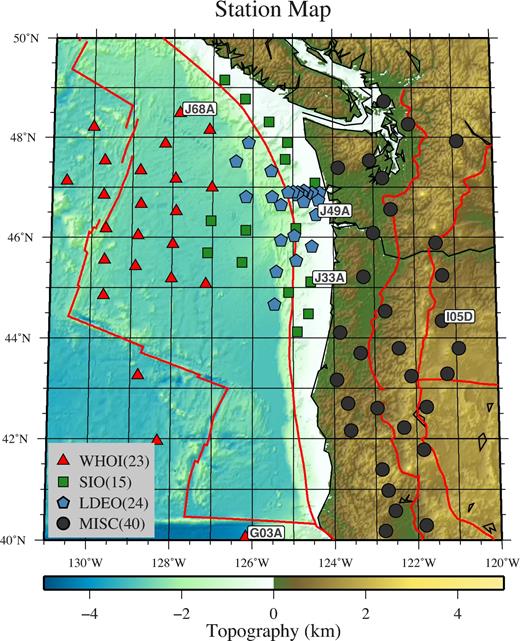
Stations used in the present study. Symbols indicate the origin of the stations from different institutions identified in the legend. Stations names are indicated for examples presented in the paper.
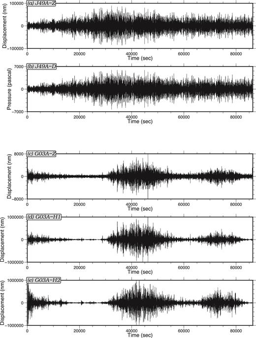
Examples of typical compliance and tilt noise for oceanic stations. Records on 2012 March 4 are plotted after applying a bandpass filter between 10 and 50 s period. (a) Vertical (Z) component of station J49A. (b) Differential pressure gauge (DPG) record for station J49A. Correlated signals between the vertical component and DPG indicate strong compliance noise. (c) Vertical component of station G03A. (d) The first horizontal component (H1) of station G03A. (e) The second horizontal component (H2) of station G03A. Large amplitudes on the horizontals are caused by local noise sources such as bottom currents. Correlated signals on the vertical and horizontal components indicate tilt noise.
Note that the coherence function is complex as defined here. Its phase is the same as the phase of the transfer function and its magnitude describes the degree to which the response channel can be predicted linearly from the source channel. In defining the compliance and tilt transfer functions the response channel in both cases is the vertical component seismometer. For compliance the source channel is the DPG and for tilt the source channel is the appropriately rotated horizontal component as discussed below.
As showed later by Figs 4 and 5, this relationship is consistent with the frequency content of the observed compliance noise and ensures the efficient removal of it.
Bell et al. (2015) also show that tilt angles can be estimated from the admittance of the tilt transfer functions and find that these angles drift continuously over time and may shift abruptly as the instrument re-levels. We, therefore, compute transfer functions using daily records after removing time windows affected by earthquakes. We partition each daily record into a maximum of forty-three 2000 s segments depending on how much time is affected by earthquakes. To minimize uncertainties in the tilt transfer function, instead of predicting noise from the two horizontal components separately, we follow Bell et al. (2015) and predict and remove the tilt noise from the horizontal component rotated in the direction of the tilt. Examples of the tilt transfer function are shown in Fig. 3, where we plot the mean and standard deviation of the horizontal-to-vertical transfer functions over the first nine days of March, 2012 for deep water station J68A (Fig. 1), which is affected by strong tilt noise. As indicated by the coherence curve, tilt noise begins to dominate at frequencies below about 0.1 Hz and extends all the way down to ∼0.002 Hz. At higher frequencies, tilt noise is more strongly affected by microseism Rayleigh waves propagating from distance sources, as indicated by the approximately π/2 phase shift between the horizontal and vertical components, which is expected for the Rayleigh wave. Tilt admittances computed on different days agree well (as indicated by the low standard deviations) and phases are close to zero whenever the coherence is high. Note that the coherence drops abruptly at 0.06, 0.077, and 0.093 Hz. The origin of these drops is not well understood. They are probably caused by instrument disturbances due to their being approximately equally spaced in frequency and they appear constantly over the whole time period studied.
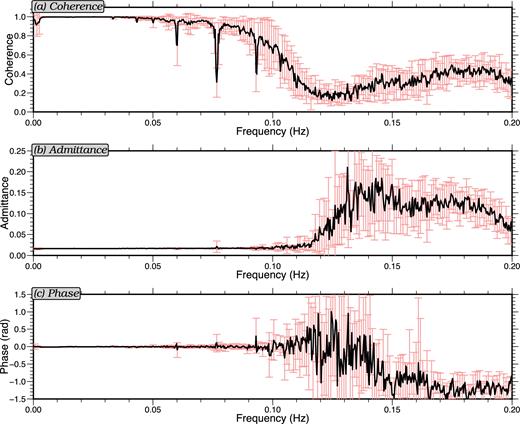
Example horizontal-to-vertical tilt transfer function for station J68A for the first nine days of March 2012. The black lines indicate the means of the transfer function characteristics over the nine days and the error bars are the standard deviations of the characteristics: (a) coherence, (b) admittance and (c) phase.
The compliance transfer functions are computed in a similar manner, but the source channel is the DPG. Fig. 4 shows the example of the mean and standard deviation of nine pressure-to-vertical compliance transfer functions for the first nine days of March 2012 for shallow water station J49A (Fig. 1). High coherence close to 1 is seen consistently between about 0.01 and 0.12 Hz. Some small variations appear on the coherence curve at lower frequencies, which are probably caused by higher tilt noise on some dates. The admittances agree well, as indicated by the low standard deviation, in the frequency range of high coherence where the observed phases are close to zero.
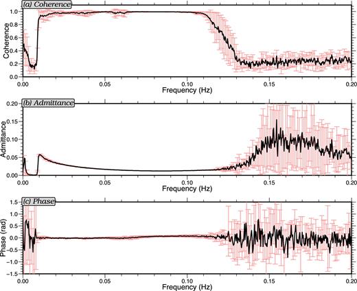
Example pressure-to-vertical compliance transfer functions for station J49A for the first nine days of March 2012. Similar to Fig. 3, black lines indicate the means of the transfer function characteristics over the nine days and the error bars are the standard deviations of the characteristic: (a) coherence, (b) admittance and (c) phase.
Tilt noise affects our ability to remove compliance noise and vice versa. To remove both we iterate. We first compute both the pressure-to-vertical and horizontal-to-vertical transfer functions on the original records for each station and each day. We then down-weight the amplitude of the coherences based on eq. (5) and compare the down-weighted coherences of the two transfer functions to decide which type of noise is stronger for the considered daily record. The predicted effect of the noise source with the stronger averaged coherence is removed first. This minimizes uncertainties in the applied transfer function (Bell et al.2015). We then re-compute the other transfer function to predict and remove the weaker noise source. The transfer functions are only applied in the frequency bands where the coherences are greater than 0.5 as discussed above. The necessity of this iterated process is illustrated later in Fig. 7.
Fig. 5 shows an example of the pressure-to-vertical compliance transfer function for 2012 March 4 for deep-water station J68A before and after the tilt noise is removed. Compliance noise is not observed on the raw transfer function (grey curves) but is revealed after the removal of the tilt noise (blue curves). As discussed earlier, due to station J68A being located in much deeper (∼2600 m) water than station J49A (∼120 m, Fig. 4), the compliance noise only appears at lower frequencies between 0.008 and 0.025 Hz. While on station J49A the compliance noise dominates the frequency band 0.01–0.12 Hz. On the other hand, a clear Rayleigh wave signal is also observed in the transfer function at and above ∼0.07 Hz (e.g. Ruan et al.2014). Computed from equation (7), the cut-off frequencies applied are 0.126 Hz for station J49A and 0.027 Hz for station J68A. As observed in Figs 4 and 5, these cut-off frequencies ensure that the compliance noise is removed completely, while also minimizing distortions to the microseism Rayleigh wave.
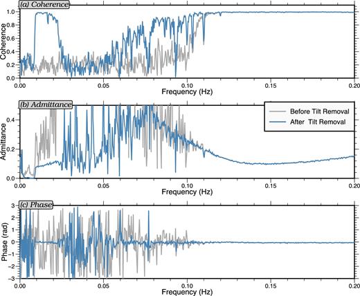
Example pressure-to-vertical compliance transfer functions for station J68A for 2012 March 4 illustrating the effect of first removing tilt noise prior to computing the compliance transfer function. Grey and blue curves are, respectively, the transfer functions before and after the tilt noise is removed. Both compliance (0.008–0.025 Hz) and Rayleigh wave (>∼0.07 Hz) signals show up clearly after tilt removal. As in Figs 3 and 4: (a) coherence, (b) admittance and (c) phase.
For stations that are affected simultaneously by strong compliance and tilt noise, a single denoising iteration does not remove both types of noise completely and a second iteration is needed. We show an example of such a case for deep-water station G03A in Figs 6 and 7. In Fig. 6, the raw vertical component daily record for 2012 March 7 is compared to the record after two denoising iterations. In the frequency band 0.05–0.1 Hz, noise is reduced by a factor of ∼7 for the peak noise and a factor of ∼1.7 on average throughout the day. In the lower frequency band 0.01–0.05 Hz, noise is reduced by a factor of ∼60 for the peak noise and a factor of ∼10 on average throughout the day. The effects of removing each type of noise on this station are shown in Fig. 7. Each dot in the figure is a daily averaged amplitude reduction value computed as the average ratio between the records before and after a specific type of noise is removed. In both the 0.05–0.1 Hz and the 0.01–0.05 Hz frequency bands, amplitude reductions of removing the tilt noise for the first time (Figs 7a and b) increase, in general, with time. This is consistent with the observation made by Bell et al. (2015) that the tilt angle on this station increases continuously from about 0.1° at the beginning to about 0.5° at the end of the time period.
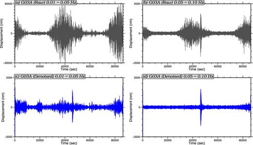
Top row: Vertical component daily record for station G03A on 2012 March 7 in two pass bands: (a) 20–100 s period and (b) 10–20 s period. Bottom row: The same records where tilt and compliance noise have been iteratively removed: (c) 20–100 s period and (d) 10–20 s period.
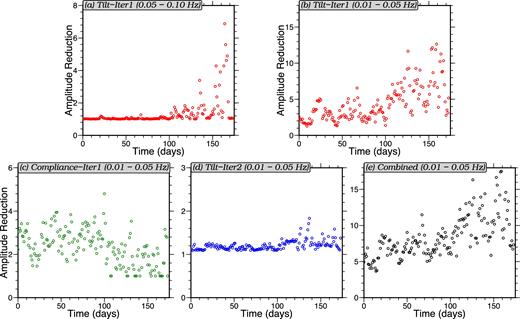
Daily averaged amplitude reduction (ratio) of the vertical component records for deep water station G03A. Each small circle in the diagrams indicates the daily averaged amplitude ratio of the record before and after the identified type of noise is removed. Horizontal axes present time in number of days where day zero is 2011 November 22, which is the first day with reasonable data for this station. (a) Amplitude reduction of removing tilt for the first iteration (10–20 s period). (b) Similar to (a), but between 20 and 100 s period. (c) Amplitude reduction of removing compliance for the first iteration (20–100 s). (d) Amplitude reduction of removing tilt for the second iteration (20–100 s). (e) Total amplitude reduction after two denoising iterations, combining the effects from (b), (c) and (d). A summary in three period bands of this total denoising statistic is presented for each station in Table 1.
The overall amplitude reductions averaged over the entire time of study are shown in Table 1 for the OBS stations. Out of the 62 OBSs listed in Fig. 1, five (FN03A, FN06A, FN09A, FN10A and FN19A) do not have three-component seismic data, seven (FN16A, J51A, J58A, J59A, M03A, M04A and M05A) do not have the normal DPG component (BDH/HDH, five out of these seven stations do, however, have substitution absolute pressure gauge components BXH/HXH that may potentially be used to apply the same noise removal technique in the future), and three (FN01A, FN05A and M02A) seem to have erroneous three-component seismic data records. This leaves 47 OBS stations, listed in Table 1, to which our denoising data processing procedure is applied.
Amplitude reductions on OBS stations in three frequency bands.
| Station | Longitude | Latitude | Depth (m) | 0.01–0.05 Hz | 0.05–0.10 Hz | 0.10–0.20 Hz |
|---|---|---|---|---|---|---|
| J57A | 235.549 | 47.0801 | 59 | 23.3 | 28.9 | 6.37 |
| J49A | 235.572 | 46.4378 | 123 | 21.0 | 24.4 | 1.25 |
| J25A | 235.378 | 44.4729 | 157 | 32.4 | 54.5 | 1.02 |
| J41A | 235.463 | 45.8119 | 174 | 23.6 | 39.3 | 0.98 |
| FN07A | 235.214 | 46.8555 | 175 | 48.4 | 67.8 | 1.03 |
| M08A | 235.105 | 44.1187 | 184 | 32.1 | 40.3 | 1.21 |
| J73A | 233.808 | 48.7677 | 187 | 26.8 | 47.8 | 1.05 |
| M01A | 233.278 | 49.1504 | 193 | 38.5 | 66.0 | 1.05 |
| J65A | 234.860 | 47.8913 | 195 | 29.1 | 63.3 | 1.00 |
| FN18A | 235.275 | 46.6998 | 212 | 25.5 | 33.5 | 0.97 |
| FN08A | 235.123 | 46.8888 | 312 | 3.62 | 5.37 | 0.95 |
| J33A | 235.429 | 45.1066 | 397 | 34.2 | 28.6 | 1.01 |
| FN12A | 234.881 | 46.8885 | 875 | 3.58 | 3.59 | 1.03 |
| FN14A | 235.035 | 46.0248 | 1012 | 30.0 | 7.63 | 1.01 |
| M06A | 235.073 | 45.5295 | 1369 | 13.7 | 18.3 | 0.99 |
| M07A | 234.883 | 44.8987 | 1467 | 10.7 | 1.03 | 1.01 |
| J42A | 234.700 | 45.9331 | 1591 | 10.5 | 1.04 | 1.01 |
| J50A | 234.701 | 46.6402 | 1742 | 8.02 | 1.12 | 1.01 |
| J34A | 234.585 | 45.3057 | 2320 | 1.23 | 1.23 | 1.00 |
| J39A | 230.356 | 46.1760 | 2437 | 2.10 | 1.10 | 1.01 |
| J31A | 230.327 | 45.5531 | 2573 | 1.90 | 1.13 | 1.01 |
| J68A | 232.171 | 48.4810 | 2584 | 9.06 | 1.81 | 0.99 |
| J67A | 232.916 | 48.1500 | 2587 | 3.62 | 1.06 | 0.99 |
| J52A | 232.984 | 46.9920 | 2629 | 1.36 | 1.09 | 0.99 |
| J43A | 233.828 | 46.1378 | 2647 | 7.01 | 0.98 | 0.98 |
| J23A | 230.317 | 44.8440 | 2649 | 7.90 | 1.31 | 1.00 |
| J54A | 231.188 | 47.3358 | 2649 | 3.02 | 1.09 | 0.99 |
| J61A | 231.803 | 47.8725 | 2662 | 2.90 | 0.99 | 0.99 |
| J35A | 233.733 | 45.4989 | 2667 | 7.73 | 0.99 | 0.98 |
| J47A | 230.286 | 46.8433 | 2677 | 3.07 | 1.11 | 0.98 |
| J53A | 232.078 | 47.1642 | 2698 | 8.54 | 1.27 | 0.98 |
| J44A | 232.961 | 46.3230 | 2719 | 5.20 | 0.98 | 0.98 |
| J55A | 230.292 | 47.5305 | 2728 | 3.21 | 1.14 | 0.99 |
| J46A | 231.212 | 46.6639 | 2748 | 5.63 | 1.39 | 0.981 |
| J45A | 232.095 | 46.5209 | 2757 | 5.54 | 1.14 | 0.99 |
| J38A | 231.147 | 46.0395 | 2774 | 3.69 | 1.06 | 1.00 |
| J30A | 231.093 | 45.4242 | 2786 | 3.90 | 1.13 | 1.01 |
| J48A | 229.349 | 47.1304 | 2820 | 1.20 | 1.02 | 0.99 |
| J36A | 232.877 | 45.6855 | 2823 | 5.72 | 0.99 | 0.98 |
| J29A | 231.992 | 45.1757 | 2834 | 3.58 | 1.13 | 0.99 |
| J63A | 229.997 | 48.2065 | 2852 | 9.55 | 1.30 | 0.99 |
| J37A | 232.015 | 45.8642 | 2862 | 1.27 | 1.03 | 0.99 |
| J26A | 234.534 | 44.6547 | 2863 | 1.21 | 1.21 | 0.99 |
| J28A | 232.844 | 45.0636 | 2876 | 8.45 | 1.31 | 0.98 |
| G30A | 231.681 | 41.9550 | 3141 | 12.9 | 2.60 | 1.00 |
| J06A | 231.199 | 43.2515 | 3183 | 8.40 | 1.16 | 1.01 |
| G03A | 233.838 | 40.0591 | 4060 | 8.17 | 1.34 | 1.00 |
In the 0.01–0.05 Hz frequency band, at the lowest frequencies, almost all the OBSs display significant noise reduction by removing the tilt and compliance noise, although noise reductions are smaller on deep water stations (>1500 m in water depth) due to weaker compliance noise. In the 0.05–0.1 Hz frequency band, noise reductions are high on shallow water stations, but are much lower on deep water stations because the compliance noise does not extend into this frequency range in the deep ocean. High noise reduction values (>1.1) on deep water stations in this frequency band indicate significant tilt noise. In the 0.1–0.2 Hz frequency band, at the highest frerquencies, only station J57A (59 m) and J49A (123 m) observe significant amplitude reductions due to them being located in exceptionally shallow water where compliance noise extends into the secondary microseism band. Rayleigh wave microseism signals dominates all other OBSs on which the denoise technique does not reduce the noise significantly in this frequency band.
Extra caution should be taken in interpreting the amplitude of ambient noise as these corrections could introduce distortions and therefore affect the relative amplitudes of cross correlations. Bell et al. (2015) discussed in detail the possible distortions of applying the compliance correction and gave a relationship between the corrected vertical component (ZC) and the true Rayleigh wave signal (ZR): ZC = ZR(1 − QW/QR), where QW and QR are, respectively, the compliance and Rayleigh wave pressure-to-vertical transfer function. It is, however, showed by Crawford & Webb (2000) and Ruan et al. (2014) that QW is much smaller (usually by one order of magnitude) than QR in the frequency band of interest for our study and, therefore, produce minimum distortion in the corrected signal. The tilt correction, on the other hand, would not cause direct reduction of the Rayleigh wave amplitude due to the expected π/2 phase shift between the vertical and horizontal Rayleigh wave components. It might still distort the vertical Rayleigh wave signal, but with a minimal effect due to the tilt admittance being much smaller than the typical value of Rayleigh wave vertical-to-horizontal ratio.
3 COMPARISON OF AMBIENT NOISE CROSS-CORRELATIONS BEFORE AND AFTER REDUCTION OF TILT AND COMPLIANCE NOISE
To investigate the effects of removing tilt and compliance noise on ambient noise cross-correlations, we compute two sets of ambient noise cross-correlations between all station pairs. For the first set, we follow a traditional ambient noise cross-correlation procedure designed for application to continental stations (Bensen et al.2007) and apply an earthquake filtered (10–40 s) running-average time domain normalization followed by spectral whitening. For the second set, we add the compliance and tilt noise removal process as described in Section 2 before the normalizations applied to the continental stations. Record sections of the shallow water station J49A are plotted in Figs 8(a) and (d) for both cross-correlation sets in two frequency bands. Between 160 and 270 daily cross-correlations are stacked for each of these station pairs. In both the 12–20 s period band and the 20–30 s period band, there is no observable signal on the raw cross-correlations using the traditional procedure (Figs 8a and c). This is consistent with the results shown by Tian & Ritzwoller (2015), where the traditional continental procedure does not produce any measurable signal on OBS pairs at and beyond 20 s period and has extremely low SNRs at 10–20 s period on most of the station pairs involving shallow water stations. Clear Rayleigh wave signals show up in both period bands, however, after removing the tilt and compliance noise (Figs 8b and d). As shown in Fig. 9, the removal of tilt and compliance noise, which we refer to as ‘denoising’, does not have as strong of an effect at periods below 10 s or above 30 s. There is, however, strong tilt and compliance noise above 30 s period, but the intrinsic ambient noise signals are weaker in this band than at shorter periods. Although the SNRs are improved in this band they remain lower than in the period band between 10 and 30 s even after denoising.
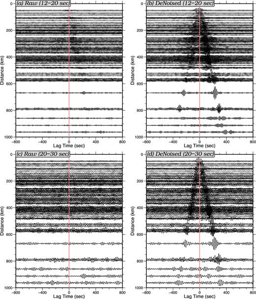
Record sections of vertical component ambient noise cross-correlations for the shallow water station J49A. A total of 160–270 daily cross-correlations are stacked for each resulting cross-correlation shown here. (a) ‘Raw’ cross-correlations computed without correcting for tilt or compliance noise, bandpass filtered between 12 and 20 s period. (b) Similar to (a), but these ‘denoised’ records have tilt and compliance noise removed. (c) Similar to (a), but filtered between 20 and 30 s period. (d) Similar to (c), but with tilt and compliance noise removed. At both period ranges the denoised records show clearer Rayleigh waves.

where σ defines the standard deviation of the Gaussian weighting function. For the results shown here, a σ of 0.1 is used, which effectively reduces to near zero the SNR measurements for group velocity measurements more than ∼20 per cent away from the reference curve, partially depresses measurements between 10 per cent and 20 per cent, and leaves measurements within 10 per cent almost unchanged.
An example of this down-weighting process is shown in Fig. 10 with measurements made on shallow water-continent station pair J33A-I05D (Fig. 1) from both cross-correlation sets, where measurements made using the traditional processing scheme are shown with red circles and the denoised measurements are shown with blue dots. The original SNR curves are peaked near 8 s period and have non-zero values across the whole period range from 1 to 35 s period. After down weighting by the group speed dispersion bias, the raw SNR curve drops to zero beyond 11 s period because of the large error of its group velocity measurement. The zero values mean, essentially, that there is no Rayleigh wave observed in the cross-correlation. Also, both curves are weighted-down below 5 s period where the measured dispersion curves begin to scatter appreciably.
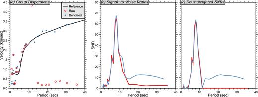
Illustration of relation between the SNR and the down-weighted SNR (DSNR) presented for the ambient noise cross-correlation between stations J33A and I05D. (a) The black line is the reference curve for this path between continental and shallow oceanic stations. Red and blue symbols indicate the group velocity measured using the cross-correlation without correcting for tilt and compliance noise and the measurements using the denoised cross-correlation, respectively. (b) The SNR curves measured base on the dispersion curves shown in (a). (c) The so-called ‘downweighted SNR’ curves which have been down-weighted according to the deviation from the measured group velocity compared to the reference curve.
The reference group velocity dispersion curve for each path is chosen based on the water depth at the station-pair used to produce the ambient noise cross-correlation. When both stations are in deep water (>1.5 km depth), the reference dispersion curve is taken from the lithospheric age dependent model of Tian et al. (2013). For all other path types (continental, continent-to-shallow ocean, continent-to-deep ocean, and shallow ocean-to-deep ocean), we construct reference dispersion curves from the average of all the dispersion measurements of the associated type. Most of the shallow ocean-to-shallow ocean paths do not have high quality signals to be measured even with the denoising process applied. The shallow ocean-to-deep ocean reference curve is, therefore, used for the shallow paths instead. Example reference group velocity dispersion curves are shown in Fig. 11. Note that the accuracy of these reference curves may degrade towards the short periods (<5 s) where the ambient noise signals weaken.
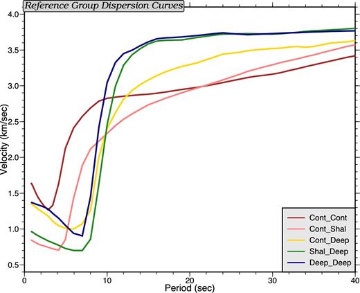
Reference group velocity curves, which are averages of measured curves between stations located in different regions: continent–continent, continent–shallow ocean, continent–deep ocean, shallow ocean–deep ocean, and deep ocean–deep ocean.
To summarize the results, for each station we compute the average of the downweighted SNRs (DSNRs) for all interstation cross-correlations involving the target station at a given period. We use this averaged DSNR (ADSNR) as an indicator of the overall quality of cross-correlations involving this station. The results computed in two different period bands are shown in Fig. 12 (12–20 s) and Fig. 13 (20–30 s). Based on a comparison of the ADSNR values to the ocean bottom station measurement qualities obtained by Tian et al. (2013) and Tian & Ritzwoller (2015), an ADSNR less than 1 indicates no measurable Rayleigh wave on that station and an ADSNR greater than 8 indicates a significant percentage of measurable Rayleigh waves on the cross-correlations. At 12–20 s period (Fig. 12), most of the shallow water stations are improved from having no measurements at all to having some measurable paths. The percentage of useful paths are improved for most deep water stations as well. At 20–30 s period (Fig. 13), almost all ocean-bottom stations benefit significantly from the denoising process. This process even affects some of the near-shore continental stations, potentially by removing horizontal noise leaked into the vertical components. Note that only 47 OBSs are plotted on the denoised maps for reasons discussed in Section 2.
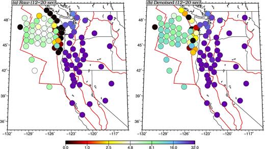
Comparison of the averaged downweighted SNRs between ‘raw’ ambient noise cross-correlations which have not been corrected for tilt or compliance noise and ‘denoised’ cross-correlations which have been corrected. The colour plotted at each station location indicates the DSNR averaged between 12 and 20 s period among all paths involving this station.
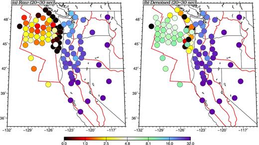
Similar to Fig. 12, but averaged in between 20 and 30 s period.
These results provide evidence of a substantial improvement in the quality of Rayleigh wave ambient noise cross-correlation measurements from 10 to 30 s period, which promises a greater utility of these measurements for ambient noise tomography. In contrast with Bowden et al. (2016) who argue that the strength of the fundamental mode Rayleigh wave is reduced due to these noise removal techniques, we find that the SNR is actually increased for the Rayleigh wave at all periods, as illustrated in Table 1 and Figs 12 and 13. We believe this difference must be related to differences in our data processing procedures relative to theirs.
4 IMPROVEMENT OF ESTIMATES OF AMBIENT NOISE DIRECTIONALITY
In the study of the location and mechanism of microseism generation, Tian & Ritzwoller (2015) analysed ambient noise directionality based on the SNRs of ambient noise cross-correlation measured using the Cascadia initiative OBSs combined with stations on the Western US continent. They found that oceanic stations are severely contaminated by local noise in the primary microseism band (10–20 s period) and are almost unusable for the directionality study for stations deployed in shallow waters. To make meaningful observations, they discarded most of the shallow water stations and averaged among station groups to stabilize the results. Here, we investigate the effect of the tilt and compliance reduction technique to improve both the accuracy and the spatial extent of the ambient noise directionality study.
In Fig. 14, we present ‘fan diagrams’ similar to those presented in Tian & Ritzwoller (2015) to summarize the strengths of the primary microseism (12–20 s period) waves propagating ‘outward’ from a single station. Each fan diagram presents a visual image of signal strength of ambient noise in different azimuthal directions, propagating outward from the station. Higher signal strengths are plotted with cool colours and lower strengths are in warm colours. A blue azimuthal sector on a fan represents strong ambient noise signals propagating from the central station to other stations in the azimuthal sector. Here, DSNRs, instead of the raw SNRs, are used to produce these fan diagrams. They are averaged between 12 and 20 s period, while the fan diagrams in Tian & Ritzwoller (2015) show peak SNRs between 11 and 20 s period. These two differences put the fan diagrams shown here on a slightly different scale from those shown by Tian & Ritzwoller (2015).
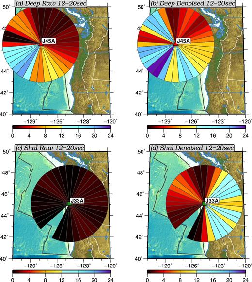
‘Fan Diagrams’ that summarize the azimuthal dependence of the amplitude of the primary microseism (12–20 s). Cooler colours indicate strong signals pointing in the direction of propagation whereas warmer colours indicate weaker signal. (a) Deep water station J45A before the removal of tilt and compliance noise. (b) Same as (a), but after the removal of tilt and compliance noise. (c) Shallow water station J33A before the removal of tilt and compliance noise. (d) Same as (c), but after the removal of tilt and compliance noise.
Figs 14(a) and (b) compares the signal strength of Rayleigh wave ambient noise in different azimuthal directions before and after the reduction of the tilt and compliance noise for a deep oceanic station J45A in the period band between 12 and 20 s. With the raw cross-correlations (Fig. 14a), where tilt and compliance noise have not been reduced, strong signals are observed to propagate to the southwest, while signals propagating towards the northwest and southeast directions are much weaker. The fan diagram after noise reduction (Fig. 14b) shows much stronger signals in these three directions in addition to stronger but still weak signals propagating toward the north, northeast, east, and southeast directions. These three directions of the strongest signals are consistent with the three potential local source regions for the primary microseisms discussed by Tian & Ritzwoller (2015).
Similarly, in Figs 14(c) and (d), we present the fan diagram comparison for shallow water station J33A, where there is almost no observable signal in the raw diagram, but reasonably strong signals are observed on the denoised diagram. A potential problem of using such shallow water stations to study ambient noise directionality, however, is the inconsistency of the noise levels on the receiver stations in the cross-correlations. For the example presented in Fig. 14(d), receiver stations at azimuths between 0° and 180° are continental while at azimuths between 180° and 360° they are oceanic stations which have much higher noise levels. This inconsistency in noise level produces a bias in the apparent signal strength towards the eastern side of the fan diagram. This either should be corrected or interpreted with caution in any study involving the SNRs of ambient noise cross-correlations.
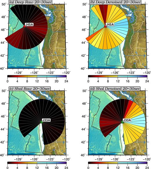
Similar fan diagrams for the secondary microseism (5–10 s) and longer periods (20–30 s) are shown in Figs 15 and 16 for the same stations. In the secondary microseism band, DSNRs improved only slightly on average after removing the tilt and compliance noise due to this period band being dominated by microseism energy rather than local noise. The strongest secondary microseism signals are observed to propagate to the east, in general, for both shallow and deep water stations, which is consistent with the observations made by Tian & Ritzwoller (2015). On the other hand, DSNRs at longer periods (20–30 s, Fig. 16) improve significantly such that the denoised fan diagrams show strong signals propagating to the east, presumably generated in deep water.
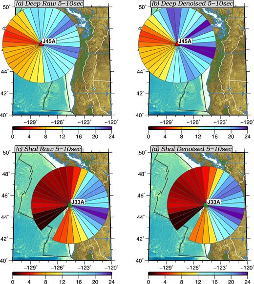
Similar to Fig. 14, but for the secondary microseism (5–10 s).
Tian & Ritzwoller (2015) showed fan diagrams across the entire JdF plate and on-shore for the primary and secondary microseism bands, but did not present results for longer period (>20 s) signals, as they are obscured by tilt and compliance noise. Here we present a map of the fan diagrams across the region at longer periods (20–30 s period) in Fig. 17 computed after the removal of the tilt and compliance noise. Three observations are worth noting: (1) Strong signals propagating, in general, to the east are observed on both the continental and oceanic stations. (2) Weaker but systematic signals propagating to the southwest are observed on continental stations, but are not observed on the OBSs. Signals with similar directionalities are observed for the primary microseism band by Tian & Ritzwoller (2015) and are believed to have originated from storms in the North Atlantic Ocean. (3) Signals propagating to the west are also observed on the OBSs, but are not observed on the continent, indicating the possible existence of source regions near the coastline at these longer periods. The source locations for this period band, however, require further study.
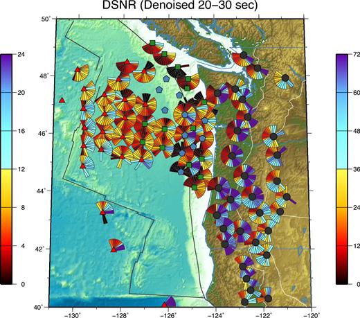
Fan diagrams at all stations between 20–30 s period. Oceanic and continental stations are plotted on different colour scales as indicated by the colour bars on the left (ocean) and right (continent). Station symbols indicate the origin of the stations from different institutions as explained by Fig. 1.
5 CONCLUSIONS
Based on 61 OBSs within the JdF plate from the Cascadia Initiative experiment and 40 continental stations in the far western United States. Consistent with Bell et al. (2015) we investigate the noise environment across the JdF plate and find that tilt and compliance noise are the major sources of local noise that contaminate the vertical channels of the OBSs. These two types of noise can be predicted and greatly reduced from the vertical component data, on a daily basis, through the horizontal-to-vertical (for tilt) and pressure-to-vertical (for compliance) transfer functions. For each daily record, we remove the type of noise that has a higher overall coherence first to minimize uncertainties. To ensure clean results, this process is applied iteratively until the average coherences of both types of noise are below 0.5. This usually means that a second iteration is applied on stations/dates that are strongly affected by both types of noise.
We compute ambient noise cross-correlations of all station pairs both before and after the tilt/compliance noise removal process to obtain two separate cross-correlation data sets for comparison. We then apply FTAN to measure the SNRs for all station pairs on both cross-correlation sets. Each of these SNRs is then down-weighted based on how much the measured group speed is biased from a reference curve. We use the ADSNR on each station as an indicator of the overall quality of the cross-correlations in which that station is involved. Almost all the oceanic stations display improved cross-correlation qualities at periods greater than 10 s after reducing the tilt and compliance noise (Table 1). In the period band between 20 and 30 s, most oceanic stations are improved from having almost no signal to having a significant number of measurable cross-correlations. These results imply improvements in both the spatial extent and bandwidth of ambient noise tomography due to the reduction of tilt and compliance noise.
We provide further evidence that the reduction of the tilt and compliance noise will improve the accuracy and the frequency and spatial extents of the microseism directionality studies based on ambient noise cross-correlations. The study of the generation of longer period microseisms (20–30 s) can be performed with the help of the noise removal technique and may provide new information about the generation mechanism of ambient noise. Corrections must be made, however, on shallow water stations to account for the inconsistency in noise levels of the receiving stations in the cross-correlations.
Acknowledgments
This research was supported by National Science Foundation grant EAR-1537868 at the University of Colorado at Boulder. The authors are grateful to the Cascadia Initiative Expedition Team for acquiring the Amphibious Array Ocean Bottom Seismograph data and appreciate the open data policy that makes these data available. The authors thank Anne Sheehan for encouragement and critical comments on an early draft of this paper. The facilities of the IRIS Data Management System were used to access all of the data used in this study. The IRIS DMS is funded through the US National Science Foundation under Cooperative Agreement EAR-0552316. This work utilized the Janus supercomputer, which is supported by the National Science Foundation (award number CNS-0821794), the University of Colorado Boulder, the University of Colorado Denver, and the National Center for Atmospheric Research. The Janus supercomputer is operated by the University of Colorado at Boulder.
