


Summary
We derive a quasi-geostrophic (QG) system of equations suitable for the description of the Earth’s core dynamics on interannual to decadal timescales. Over these timescales, rotation is assumed to be the dominant force and fluid motions are strongly invariant along the direction parallel to the rotation axis. The diffusion-free, QG system derived here is similar to the one derived in Canet et al. but the projection of the governing equations on the equatorial disc is handled via vertical integration and mass conservation is applied to the velocity field. Here we carefully analyse the properties of the resulting equations and we validate them neglecting the action of the Lorentz force in the momentum equation. We derive a novel analytical solution describing the evolution of the magnetic field under these assumptions in the presence of a purely azimuthal flow and an alternative formulation that allows us to numerically solve the evolution equations with a finite element method. The excellent agreement we found with the analytical solution proves that numerical integration of the QG system is possible and that it preserves important physical properties of the magnetic field. Implementation of magnetic diffusion is also briefly considered.
1 INTRODUCTION
The Earth’s magnetic field shows oscillations and variations on a wide range of temporal scales (Hulot et al.2015). This variability is the observable consequence of the rich dynamics taking place in the Earth’s outer core, where the geomagnetic field is generated and continuously altered by the complex interplay between fluid flows and the geomagnetic field itself (Jackson & Finlay 2015; Roberts 2015).
Numerical geodynamo models (Christensen & Wicht 2015) can capture qualitative features of the geomagnetic secular variation and of the spatial structure of the geomagnetic field at the core–mantle boundary (CMB) but the whole temporal spectrum is impossible to cover due to the prohibitive computational costs required. For the same reason, current numerical simulations operate in a parameter regime that is far away from what is thought to be the one in which the geodynamo operates. For instance, the ratio of the rotation to viscous timescales, as measured by the Ekman number Ek, is supposed to be extremely small in the Earth’s core for which Ek = O(10−15). Recent numerical simulations (Schaeffer et al.2017) are capable of reaching Ek = O(10−7) suggesting that they might not operate in the same regime as the true geodynamo. Conversely, according to Aubert et al. (2017), these simulations might be in the correct asymptotic regime. In the same paper, the authors present the results from simulations where the value Ek = 10−8 has been reached with hyperdiffusivity applied to the smallest length scales. The ratio of magnetic to viscous dissipation timescales, as measured by the magnetic Prandtl number Pm is also orders of magnitude higher in numerical simulations than in the core: Pm = O(10−5–10−6) in the core while Pm > 3 × 10⁻² in recent simulations (Aubert et al.2017; Schaeffer et al.2017). These numbers indicate that the enormous spatial and temporal scale separation that is thought to be characteristic of the dynamics in the core is not present in numerical models. Unfortunately, by lowering Pm it becomes more difficult to obtain self-sustained dynamo simulation, as clarified by the relationship Rm = PmRe between the Reynolds number Re (a measure of the vigour of the flow velocities) and the magnetic Reynolds number Rm. Since the latter has to overcome a certain critical value for dynamo action to take place, one can see how lowering Pm to Earth-like values tends to result in the generation of weaker magnetic fields. Therefore stronger fields require more vigorous flows and consequently additional computational burden. As a consequence, geodynamo simulations typically have a lower ratio of magnetic to kinetic energy (less than 10) than what it is believed to be relevant for the Earth (where this value is about 100). See Schaeffer et al. (2017) for a summary of recent geodynamo simulations and for their comparison with the Earth’s dynamo.
A possible route towards the development of numerical models capable of operating in more realistic parameter regimes is given by a class of models that attempts to represent only the physics that is thought to be relevant for the Earth’s core. In particular, models based on the quasi-geostrophic (QG) approximation take advantage of the smallness of the Ekman and Rossby (Ro) numbers, the latter being a measure of the importance of inertia over rotational forces. These non-dimensional numbers are an indication of how rotation (via the Coriolis force) is dominant in the force budget of the core. As such the Earth’s core is said to be in rapid rotation. The fluid flows characteristic of such a system are essentially 2-D, with vertical component strongly inhibited by the presence of rotation, as predicted by the Proudman–Taylor theorem (Greenspan 1968; Jacobs 1987). Even when magnetic and thermal effects are included (by including in the momentum equation the Lorentz force and buoyancy, respectively) flows retain their columnar structure (vertically invariant), as long as the main balance remains geostrophic, that is, a balance between pressure gradient and the Coriolis force. The remaining forces, most notably inertia, Lorentz force and buoyancy, enter the balance at subdominant order, together with the Coriolis and pressure forces due to ageostrophic flows (Gillet et al.2011; Calkins et al.2015). An account of the experimental and numerical evidence for bidimensionality in rapidly rotating flows is given in Cardin & Olson (2007) and Williams et al. (2010).
These theoretical arguments, together with experimental and numerical evidence suggest that it is acceptable to impose a flow structure that is almost invariant along the vertical direction. This approach has been originally developed for studies of thermal convection (Cardin & Olson 1994; Aubert et al.2003; Gillet & Jones 2006; Guervilly & Cardin 2016) and has subsequently been used for studies of kinematic dynamos (Schaeffer & Cardin 2006; Schaeffer et al.2016), the study of interannual and decadal dynamics in a data assimilation framework (Canet et al.2009) and the study of magneto-hydrodynamic oscillations in the Earth’s core (Canet et al.2014; Labbé et al.2015). The columnar flow approximation has also been successfully applied to the inversion of geomagnetic data for the retrieval of the flows at the surface of the core (Pais & Jault 2008; Gillet et al.2009, 2015).
The use of the columnar flow approximation for the study of interannual and decadal dynamics has been justified in Jault (2008) and Gillet et al. (2011) where an impulsive perturbation of the inner core boundary (ICB) propagated into the exterior shell of a 3-D numerical model of a rotating fluid permeated by a magnetic field. These transient motions are shown to be highly columnar provided that magnetic forces do not become dominant with respect to rotation and that the disturbances propagate on timescales much shorter than the magnetic diffusion timescale and much longer than the rotation period of the shell. In the Earth’s core the propagation timescales of magnetic disturbances (the Alfvén velocity) across the core is thought to be of the order of 6–8 yr (Gillet et al.2010, 2015) and the magnetic diffusion timescale can be estimated to be at least 104 times this value (see Canet et al. (2014) and references therein). It is safe to assume that, in the Earth’s outer core, interannual and decadal flows and fluctuations are columnar. Examples of such motions include Alfvén torsional waves (Braginsky 1970) that propagate on the Alfvén timescales mentioned above, and slow magneto-hydrodynamic oscillations (Hide 1966; Malkus 1967; Finlay 2011) that, depending on the geometry and intensity of the magnetic field in the core, could move on decadal to centennial timescales and therefore be a possible mechanism for the westward drift observed in magnetic field models (Hide 1966; Finlay & Jackson 2003; Jackson 2003). The detection of these motions in 3-D geodynamo numerical simulation has proven challenging, mainly due to the high values of Ek and Pm (Teed et al.2014; Hori et al.2015). Additionally, care has to be taken in relating the observation of interannual and decadal magnetic driven oscillations to their counterpart detected in geodynamo simulations, as the timescales are likely to be not in the correct ratio with rotational or advective timescales. As both input parameters (like Ek and Pm) and diagnostic quantities (such as the ratio of magnetic to kinetic energy) in current simulations are not the same as for the Earth’s core, so are the relative timescales (Glatzmaier 2002) of relevant phenomena. In particular the ratio of the Alfvén timescale to the convective turnover or to the rotational timescale tend to be smaller in simulations than in the Earth so that equating one timescale to Earth’s values, makes other ones wrong. These issues may be also tackled by QG models currently under development.
In the present study we consider a variation of the QG model of Canet et al. (2009). The key aspect of that study is that the magnetic field is considered through vertical averages of quadratic combinations of its equatorial components. In this way both the momentum and the induction equations are projected on the equatorial plane and a fully 2-D model is obtained. The properties of the model of Canet et al. (2009) have not yet been fully characterised through a numerical simulation of the system, but data assimilation experiments have been performed in simplified settings. Subsequent QG models of magnetohydrodynamic oscillations (Canet et al.2014; Labbé et al.2015) have assumed that the magnetic field too could be approximated as columnar, with the vertical component of the field being either negligible or linearized along the vertical direction. This approximation is more restrictive than the general description of Canet et al. (2009), in which no assumption about the vertical structure of the magnetic field is made, but it allows the consistent inclusion of magnetic diffusion and the natural imposition of insulating boundary conditions at the CMB. Both these issues are addressed in the present study.
We perform kinematic forward numerical simulations of a system of equation similar to the one of Canet et al. (2009), the most notable differences being the use of a velocity formulation that enforces mass conservation (Schaeffer & Cardin 2005) and the use of vertically integrated magnetic quantities instead of vertically averaged ones to describe the magnetic field. In addition, the presence of the inner core is neglected from now on. We made this choice to simplify our study and to focus attention on the significant aspects of the QG model that we now derive. In Canet et al. (2009) and Canet et al. (2014) the magnetohydrodynamic equations are solved only outside the tangent cylinder, the imaginary cylinder aligned with the rotation axis of the Earth and tangent to the inner core and separating the regions above and below the inner core from the rest of the outer core. Whether the geostrophic balance or the columnar flow approximation hold in the fluid regions inside the tangent cylinder is an open question. In Canet et al. (2009, 2014), these regions are completely excluded from the QG dynamics on the basis that, if the flows are indeed vertically invariant outside the tangent cylinder little feedback is expected from the fluid regions above and below the inner core. A full sphere represents the simplest canonical system to study and the correct geometry for an early Earth, in which the inner core is not yet present, and some experimental configurations. As prescribed velocity field we chose a time-independent zonal flow with a cylindrical radial dependence. As we show later in the paper, this choice allows significant simplifications in the governing equations and the derivation of a relatively simple analytical solution. We do not expect the fundamental conclusion of our study to vary for more complex flows (such as non-axysimmetric flows). In Section 2, the system of equations under the QG approximation is derived and its peculiar characteristics discussed. In Section 3, we illustrate the ideal kinematic setup and the criteria chosen to validate the QG equations. By imposing a time-invariant velocity field we can study specific properties of the model in a highly simplified setup. The results of the validation are given in Section 4. In Sec-tion 5, we propose an alternative to magnetic diffusion, not possible to implement consistently in the model we derive here. Comments and conclusions are given in Sections 6 and 7.
2 GOVERNING EQUATIONS
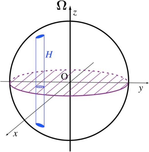
Geometry of a quasi-geostrophic column in a full sphere. H is the half height of the column, x = s cos ϕ and y = s sin ϕ, s is the distance from the rotation axis and ϕ is the azimuth.
In what follows we revisit the derivation of the governing equations for a QG model that follows closely that of Canet et al. (2009). The quasi-z invariance of the flow suggests that the dynamics can be projected on the equatorial plane and a 2-D system can be solved in place of the original 3-D described by eqs (8)–(10). The treatment of the magnetic field requires special care as in general its vertical structure is unconstrained.
2.1 Columnar flow assumption and vertically integrated equations
3 VALIDATION UNDER THE KINEMATIC APPROXIMATION
The QG equations derived in the previous section can in principle be evolved forward in time from a given initial condition. Apart from simple experiments performed in Canet et al. (2009), there has been no characterization of the property of the system (24)–(27) through forward numerical simulations. In the remainder of the paper we present results of forward numerical models under the kinematic approximation. Although the QG model discussed here is targeted to magnetic fields and flows with interannual and decadal temporal variability, we impose a steady velocity field so that we can ignore the momentum equation and focus on solving the induction eqs (25)–(27). As we are neglecting the momentum equation, we follow Jones (2007) and consider typical values of velocity in the outer core to be U = 5 × 10⁻⁴ m s−1 ≃ 15 km yr−1 which result in a non-dimensional timescale of |$r_c/\mathcal {U}=220$| yr. These timescales lie at the upper limit of validity of the QG model developed here.
3.1 Initial field and prescribed flow
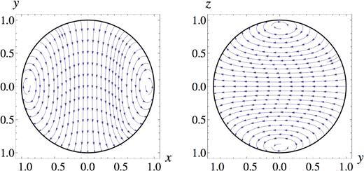
Initial magnetic field for the kinematic analysis of the QG model. The left and right panels show a projection on the x, y plane (the equatorial plane) and the right panel is a meridional cut in the z, y plane, respectively.
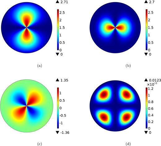
Initial conditions for (in order from panels a to d) a, b, c and q2 calculated from the initial magnetic field of Fig. 2. Maximum and minimum values are shown at the top and at the bottom of the colour scale for each quantity.
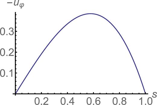
Radial structure of the zonal flow (39).
3.2 Numerical experiments setup
To assess the quality of the forward modelling, we evolve eqs (40)–(42) forward in time with the finite element method, commercially available software COMSOL Multiphysics.2 The reason for this choice is twofold. First of all, we are interested in validating the QG equations for which there is almost no phenomenological knowledge. Therefore, since at this stage high performance is not required, we decided not to develop a customized code but to use an available, flexible software preferably with the possibility of testing various types of spatial discretization and time-stepping techniques. The second reason is that the finite element method is local in nature. We are mainly concerned with the positivity of a and b and, assuming that eqs (40)–(42) actually can preserve this property with time, there is always a risk that numerical noise generates spurious negative values. This is particularly true considering that we neglected diffusion. A local method should ensure that any numerical artefacts remain localized in space, while in a global method, such as a spectral one, there is no such guarantee.
In particular we are interested in preserving positivity of a, b and q2. The quantities we compute in order to establish the performance of the model are:
- The equatorial (non-dimensional) magnetic energyThe integral on the right-hand side is calculated over the surface of the equatorial disc. In general, we do not have information about the vertical component of the magnetic field, so we can only calculate the equatorial component of the magnetic energy. However, in the simple case we are studying here the vertical component of the magnetic field does not contribute to the evolution in time of the 3-D magnetic energy evaluated over the whole core. So Em represents the time varying part of the total magnetic energy of the system and its evolution equation is(48)\begin{eqnarray} 2E_m=\int _{{\rm core}}\left(B_s^2+B_\phi ^2\right) {\rm d}V= \int _{{\rm disc}} (a+b)\,{\rm d}S. \end{eqnarray}(49)\begin{eqnarray} \frac{\partial E_m}{\partial t}=\int _{\rm disc} s c \frac{\partial }{\partial s}\left(\frac{u_\phi }{s}\right) {\rm d}S. \end{eqnarray}
- Knowing the theoretical solutions for q2 we can compute the domain integrals of the misfitwhere the theoretical solutions are of the form (45). A similar calculation can be performed for a, b and c. Here, however, we mainly focus on the deviations of the numerical solution of q2 from its analytical form since, as we show below, this is the quantity that is most prone to numerical noise.(50)\begin{eqnarray} {\rm mean}\left(q^2-q^2_T\right)=\int _{\rm disc} |q^2-q^2_T| {\rm d}S \end{eqnarray}
The minimum values of q2, a and b. Since these must be always positive quantities their minimum value should always be greater than zero.
In COMSOL, we must choose several parameters to tune the numerical method, the most significant of which are the number of mesh elements used to discretize the spatial domain and the type and degree of the polynomials we use to discretize the functions representing the variables solved on the mesh. The mesh refinements range from extremely coarse to extremely fine (see Table 1), each of which is assigned an index: the lower the index, the finer the mesh. As for the discretization inside each element, we use Lagrange polynomials with variable degree from 1 to 3. The models are identified with the nomenclature LlNn where L is the degree of the polynomials used and N is the mesh identifier. So the model run with L = 2 and N = 1 will be called L2N1. Since by choosing a coarser mesh and a high degree L the finite element method tends towards a spectral method, we decide to keep L low and use fine meshes.
3.3 Cartesian formulation
As COMSOL allows great flexibility in the choice of the domain, its algorithms are formulated in Cartesian coordinates. As such any discretized physical field in the appropriate coordinate system is always smooth and differentiable everywhere on the domain. However, considering the geometry of the system, eqs (25)–(27) have been formulated in polar coordinates and an artificial singularity has been introduced at s = 0 (Lewis & Bellan 1990). This is evident in Figs 3 where the values of a, b and c are non-unique in ϕ as s vanishes. In Cartesian coordinates, sharp gradients develop near the origin and evolving eqs (40)–(42) in COMSOL results in significant numerical noise around s = 0 (not shown here). As a result, spikes of positive and negative values of similar magnitude appear to be generated in the field q2, creating a violation of the Cauchy–Schwarz inequality that increases with time. At t = π/2 the quantity q2 locally reaches the minimum value of −1.17. Considering that q2 should always be positive and given its maximum expected value (see Fig. 3d), this violation of positivity is totally unacceptable.
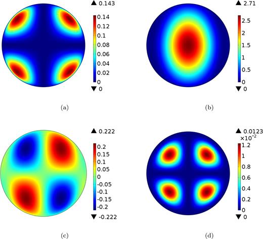
Initial conditions for (in order from panels a to d) A, B, C and q2 calculated from the initial magnetic field of Fig. 2. Maximum and minimum values are shown at the top and at the bottom of the colour scale for each quantity.
4 RESULTS
Different simulations have been run over the window 0 ≤ t ≤ π. The simulations have been performed changing the mesh refinement (mesh 1 or mesh 0) and the degree of the Lagrange polynomials. The comparison between some of these simulations is shown in Fig. 6. The magnetic energy shows that the numerical simulations have reached convergence with very small variations detectable only toward the end of the computation time interval. In Figs 7 and 8, the solution for the model L2N0 is plotted at t = 3π/4. The quadratic fields A, B and C are growing in time, each reaching values of the order 10 at the end of the simulation. Remember that q2 is not a variable solved in the simulation, it is a derived value: q2 = AB − C2. Namely, it is a small quantity (of the order 10−4) derived from a difference from bigger quantities. In this sense it is a ’weak’ point of the simulation, difficult to keep smooth, as the snapshots of Fig. 8(d) shows. The relative amplitude of the numerical fluctuations is anyway small if we compare it to the magnitude of the quadratic fields themselves, of the order of 0.001/10 = 10−4 in the L2N0 simulation, and even smaller in the L3N0 ones. The same order of magnitude holds for the negative value in q2 developing at the end of the simulation. This is the amount by which the Cauchy–Schwarz inequality is violated. Looking at A and B one can see that this is also the ratio between the most negative and positive values, expressing somehow the relative strength of positivity violation. In Fig. 9, we plot the logarithm of the absolute differences between the numerically calculated a, b, c and q2 and their analytical solutions given in eqs (44)–(47). As already pointed out the departures from the analytical solutions are very small compared to the magnitudes of the quadratic fields calculated.
The magnitudes of the misfits and violations of the positivity and Cauchy–Schwarz inequality depend on the spatial discretization adopted, as is clear from Fig. 6. Provided that the numerical model has enough degrees of freedom we argue that we managed to successfully solve the kinematic problem, with acceptable departures from the expected solution. Further refinement of the spatial grid and more accurate choices of the time stepping technique might result in more refined models capable of better performance than the ones illustrated here. We were not interested in obtaining a truly advanced numerical model but only in studying the possibility of integrating the kinematic equations forward in time. Our attention was focused on the open questions highlighted in Section 3 regarding the conservation of positivity and of the Cauchy–Schwarz inequality. Interestingly we found that the eqs (25)–(27) might not be adequate to solve the kinematic problem using a local numerical strategy due to numerical noise developing at the point s = 0. The reformulation of the problem in Cartesian coordinates, leading to eqs (56)–(58) removes this issue, providing numerically acceptable solutions. In the spherical shell geometry considered by Canet et al. (2009), where the equations are not solved near the origin, this strategy might not be necessary.
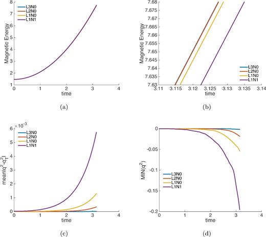
Performance comparison between different models in the ideal case. The nomenclature is LlNn where l is the degree of the Lagrange polynomial used as basis function and n is the number associated with the mesh. (a) Magnetic energy (48). (b) Zoom-in of magnetic energy towards the end of the computational interval. (c) Averaged difference between the numerically calculated q2 and the analytical solution |$q_T^2$|, according to eq. (50). (d) Minimum value of q2.
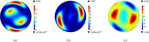
Numerical solution for the kinematic study for the diffusion free case. Variables (in order from panels a to c) A, B and C, respectively, in the diffusion free case at the instant t = 3π/4. The flow is given in eq. (39) and the initial condition in Fig. 5. The spatial mesh is the N = 0 mesh of Table 1 and the Lagrange polynomials are of degree 2. Maximum and minimum values are shown at the top and at the bottom of the colour scale for each quantity.
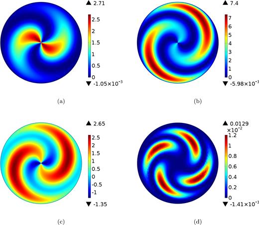
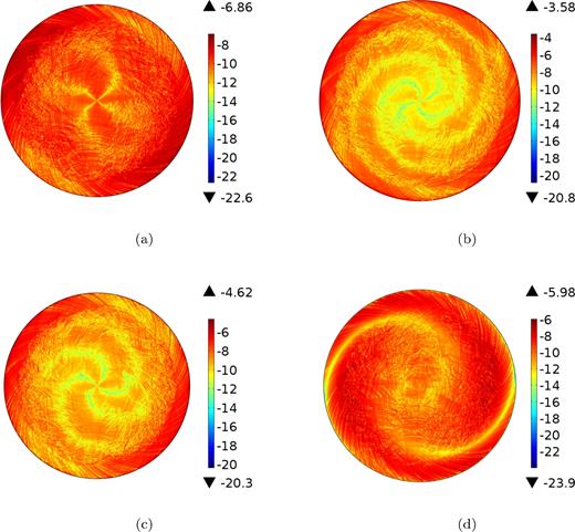
Numerical solution for the kinematic study for the diffusion free case. Variables (in order from panels a to d) a, b, c and q2 respectively, in the diffusion free case at the instant t = 3π/4. The fields have been calculated from the numerical solutions for A, B and C according to the formulae (54). The flow is given in eq. (39) and the initial condition in Fig. 3. The spatial mesh is the N = 0 mesh of Table 1 and the Lagrange polynomials are of degree 2. Maximum and minimum values are shown at the top and at the bottom of the colour scale for each quantity.
Departure of a, b, c and q2 from the true analytical solutions aT, bT, cT and |$q_T^2$|, respectively, for the diffusion free case. Shown is the logarithm of the absolute difference as a function of space for the instant t = 3π/4. The fields a and q2 are calculated from the fields A, B and C according to the formulae (54). The spatial mesh is the N = 0 mesh of Table 1 and the Lagrange polynomials are of degree 2. Maximum and minimum values are shown at the top and at the bottom of the colour scale for each quantity.
5 IMPLEMENTING DIFFUSION
We performed simulations with Rm = 101, 102 and 103. As for the diffusion free case, we integrate in time eqs (71)–(73) and we calculate the quantities a and q2 from A, B and C. The results for models L1N0 and L2N0 are shown in Figs 10 and 11. As expected the magnetic energy growth with time is slower with lower values of Rm, corresponding to higher values of the damping coefficient. However, the difference is modest for Rm up to 100. The solution is visually similar to the diffusion free case, with the damping introducing the expected effect of lowering the magnitude of both the kinematic solution and of the numerical artefacts. The misfit between q2 and |$q^2_T$| shown in Figs 10(c) and 11(c) decreases with increasing damping because all fields are damped, and so is the error. The relative errors and the relative magnitude of the negative features with respect to the amplitude of the solution is similar to the diffusion free case and so is the location of the artefacts.
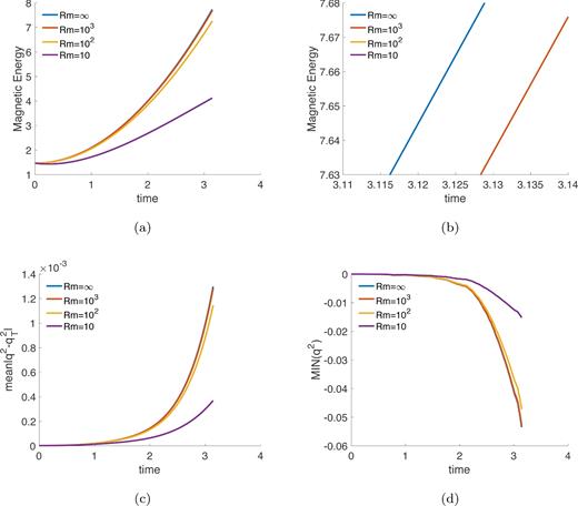
Comparison between different kinematic numerical solutions for the L1N0 model in presence of damping. Different values of Rm are considered, Rm = ∞ corresponding to case with no damping. (a) Magnetic energy (48). (b) Zoom in of magnetic energy toward the end of the computational interval. (c) Averaged difference between the numerically calculated q2 and the analytical solution |$q_T^2$|, according to (50). (d) Minimum value of q2.
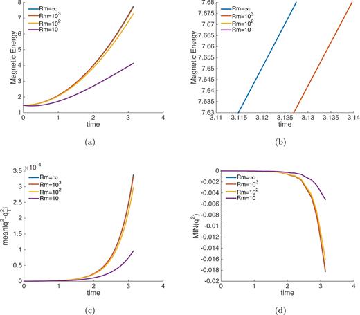
Comparison between different kinematic numerical solutions for the L2N0 model in the presence of damping. Different values of Rm are considered, Rm = ∞ corresponding to case with no damping. (a) Magnetic energy (48). (b) Zoom in of magnetic energy towards the end of the computational interval. (c) Averaged difference between the numerically calculated q2 and the analytical solution |$q_T^2$|, according to eq. (50). (d) Minimum value of q2.
6 DISCUSSION
7 CONCLUSIONS
In this study we presented a kinematic study of a QG model that is tailored to the study of the interannual and decadal dynamics of the Earth’s outer core. In Section 2, we discussed how the QG formalism arises from the 3-D magneto-hydrodynamic governing equations. Under the hypothesis of fast rotation, the columnar flow assumption is the key to developing realistic numerical models that have the potential to reach parameter regimes much closer to the real Earth than 3-D numerical models. The key operation is the projection of the governing equations on the equatorial disc. This operation is far from trivial when applied to the momentum equation, as it requires assumptions and delicate mathematic manipulations on the terms describing the body forces (Lorentz force and buoyancy in geodynamo simulations). The formulation presented in Sec-tion 2.1 has the advantage, compared to the QG formulation of Canet et al. (2014) and Labbé et al. (2015), of handling the magnetic field under very general assumptions. This is achieved by representing the magnetic field via the quadratic quantities |$B_s^2$|, |$B_\phi ^2$| and BsBϕ projected on the equatorial disc. We call this the quadratic formulation. The resulting equations are however much more complicated and magnetic diffusion is impossible to accommodate. Compared to the vertically averaged formulation of Canet et al. (2009), the equations presented here, based on a vertically integrated formulation, have the advantage of providing a natural boundary condition for the quantities a, b and c. The equations for the vertically averaged formalism can be derived from (24)–(27) dividing them by 2H.
The QG model developed here, although based on the formulation proposed in Canet et al. (2009), has never been integrated in time. Our kinematic formulation highlighted some deficiencies in the equations in polar coordinates that we removed when developing a novel Cartesian formulation.
We investigated the effect of damping as an alternative to diffusion. The simple damping term introduced in the induction eq. (66) leads to a system of equation that is now closed in a, b and c. We find that this simple solution is efficient in lowering the amplitude by which the positivity of a, b and q2 is violated.
In future studies it is necessary to characterize the full system (24)–(27) where the Lorentz force provides a link between the evolutions of the magnetic field and the fluid flows. A first step could be the calculation of magnetohydrodynamic normal modes in a similar study to those of Canet et al. (2014) and Labbé et al. (2015). In such studies care has to be taken in testing the effect of the approximations that led to the derivation of (24), namely the assumption that surface terms can be neglected compared to the vertically integrated ones. The discarded surface terms could be of importance at the equator, where the height H of the domain vanishes and singularities may compromise the derivation if not treated carefully.
Finally we point out how the use of the axial vorticity eq. (18) could not be the best option to describe the evolution of the stream function Ψ under the columnar flow approximation (15). In Labbé et al. (2015), an alternative formulation is proposed that improves the predictions of the momentum equation in the equatorial regions s ≃ 1. This technique allowed Labbé and co-authors to calculate hydrodynamic solutions that are in better agreement with 3-D calculations than previously known QG calculations (Canet et al.2014). In future work, the axial vorticity eq. (24) should therefore be replaced with an equation that is derived following the methodology of Labbé et al. (2015).
The final goal of the QG studies such the one presented here is the derivation of a numerical model capable of simulating the Earth’s core dynamics in a realistic parameter regimes. Such a model will allow the implementation of data assimilation systems that, making use of modern geomagnetic observations, could open a window on the core that has never been achieved with 3-D models. A first step toward this goal is to perform closed loop data assimilation experiment the kinematic system (25)–(27), similarly to the ones presented in Canet et al. (2009). After the momentum eq. (24) has been confidently integrated forward in time, data assimilation experiments similar to the ones performed in Fournier et al. (2013) can be attempted.
Types of meshes used in COMSOL Multiphysics for the kinematic study. The domain to be discretized is the equatorial disc. ‘tri’ indicates the number of elements used to discretize the bulk of the domain. ‘edg’ indicates the number of edge elements, or curved elements used to represent the boundary of the domain.
| Mesh identifier (N) | Mesh name | tri | edg |
|---|---|---|---|
| 0 | Custom 1 | 192 732 | 900 |
| 1 | Extremely fine | 24 934 | 316 |
| 2 | Extra fine | 6534 | 160 |
| Mesh identifier (N) | Mesh name | tri | edg |
|---|---|---|---|
| 0 | Custom 1 | 192 732 | 900 |
| 1 | Extremely fine | 24 934 | 316 |
| 2 | Extra fine | 6534 | 160 |
Acknowledgments
This study has been supported by the ETH grant number ETH-1412-1 and by the SNF grant number 200020_143596. We wish to thank Dr Dominique Jault (Université Grenoble Alpes) and Dr Elisabeth Canet (former ETH) for fruitful discussions and useful suggestions. We also wish to express our gratitude to an anonymous reviewer whose comments and suggestions greatly improved the quality of the original manuscript.
These equations correct errors in the equations given in Jault & Finlay (2015). The vertically averaged formulation employed there can be retrieved by dividing eqs (25)–(27) by 2H. Note that eqs (66) of Jault & Finlay (2015) would be formally correct for the vertically integrated formulation of the present study. The interested reader is referred to section 4.2.4 of Maffei (2016) for additional details.
