


Abstract
We investigated the shallow structure of the Solfatara, a volcano within the Campi Flegrei caldera, southern Italy, using surface waves as a diagnostic tool. We analysed data collected during the RICEN campaign, where a 3-D active seismic experiment was performed on a dense regular grid of 90 m × 115 m using a Vibroseis as the seismic source. After removal of the source time function, we analysed the surface wave contribution to the Green's function. Here, a 1-D approximation can hold for subgrids of 40 m × 40 m. Moreover, we stacked all of the signals in the subgrid according to source–receiver distance bins, despite the absolute location of the source and the receiver, to reduce the small-scale variability in the data. We then analysed the resulting seismic sections in narrow frequency bands between 7 and 25 Hz. We obtained phase and group velocities from a grid search, and a cost function based on the spatial coherence of both the waveforms and their envelopes. We finally jointly inverted the dispersion curves of the phase and group velocities to retrieve a 1-D S-wave model local to the subgrid. Together, the models provided a 3-D description of the S-wave model in the area. We found that the maximum penetration depth is 15 m. In the first 4 m, we can associate the changes in the S-wave field to the temperature gradient, while at greater depths, the seismic images correlate with the resistivity maps, which indicate the water layer close to the Fangaia area and an abrupt variation moving towards the northeast.
1 INTRODUCTION
This study is aimed at imaging the shallow structure of the Solfatara, one of the craters in the Campi Flegrei large volcanic caldera located in southern Italy, near the city of Naples. The volcanic structure of Campi Flegrei was mainly determined by two major historic eruptions: the Campanian Ignimbrite (39 kyr) and the Neapolitan Yellow Tuff (15 kyr), which created most of the present landscape of the region (Di Vito et al.1999; Pappalardo & Mastrolorenzo 2012). After these two main events, dozens of smaller eruptions affected the area, the last of which was the 1538 Monte Nuovo eruption (Guidoboni & Ciuccarelli 2011). The area is also characterized by strong bradyseism. During the last century, three main episodes occurred in the area (1950–1952, 1969–1972, 1982–1984), with the most recent resulting in an uplift of about 1.80 m (Del Gaudio et al.2010).
The deep structure of this caldera is mainly known through seismic imaging methods that have been obtained from both active and passive data (Judenherc & Zollo 2004; Vanorio et al.2005; Zollo et al.2008). Analysis of reflected waves by the amplitude versus offset technique revealed two distinct interfaces beneath Campi Flegrei (Zollo et al.2008). The deeper of these is located at a depth of ∼8 km, and is characterized by a strong increase in the Vp/Vs ratio. This was interpreted as the deep magma layer that feeds the caldera and that is responsible for eruptions in the area. This interpretation is consistent with geochemical investigations on melt inclusions from Campi Flegrei shoshonites (Mangiacapra et al.2008). The shallow interface is at ∼3 km in depth, and is instead associated with a discontinuity between the older caldera deposits and a fluid-saturated metamorphic rock layer (Zollo et al.2008), which can provide a shallow magma chamber before medium- or small-scale eruptions. This interface also separates the shallow hydrothermal system from the deeper magmatic one. The root of the bradyseism is commonly associated with this shallow layer, and has been ascribed to the intrusion of magma (D'Auria et al.2015; Trasatti et al. 2015) or to the deformation of a concrete-like caprock due to the high pressure of the underlying gases (Vanorio & Kanitpanyacharoen 2015).
The shallow hydrothermal system of the Campi Flegrei is associated with the interaction of meteoric water and the heat and fluid transfer from greater depths. Within the hydrothermal system, the Solfatara is assumed to be the top of a hydrothermal plume (Chiodini et al.2001) and it experiences large episodes of degassing, with very intense emissions of hydrothermal–magmatic gases and high heat flow (Chiodini et al.2001). The Solfatara is a crater of about 0.6 km in diameter that is bounded by normal faults, along which geothermal fluids can ascend (Bianco et al.2004). The surficial expression of these pathways are the fumaroles that are located within or at the boundaries of the crater. Several geophysical analyses have investigated the shallow structure of the Solfatara, including seismic (Bruno et al.2007), resistivity (Byrdina et al.2014) and magnetotelluric (Siniscalchi et al.2015) surveys. Tomographic images have revealed a very complex structure, with alternation of positive and negative resistive bodies, which indicates the presence of water separated by gas sacks. Additionally, ambient noise was recorded in the crater from three-component stations and data were inverted to retrieve the phase velocity of the Rayleigh waves (Petrosino et al.2012). Stable features are obtained in the frequency range 2–15 Hz; when retrieving the S-wave model from modelling of the dispersion curves, the resulting penetration depth is several tens of metres. A very shallow analysis based only on the measurement of group velocities of Rayleigh waves was also performed in the Fangaia mud pool using surface waves (Letort et al.2012), which revealed a penetration depth of a few metres.
The shallow structure below the Solfatara is also subjected to seasonal changes due to variations in the meteoric contribution to the hydrothermal system (Chiodini et al.2007). Over the last several years, the Solfatara has also experienced increases in pressure, temperature and heat flow, and significant changes in the composition and pattern of the degassing, and in its distribution through the vents (Chiodini et al.2011). Over the same period, a new uplift started after 20 yr of subsidence, with sporadic episodes of shallow seismicity beneath the Solfatara (at depths between 2 and 3 km; D'Auria et al.2015).
To provide high-resolution images of the structure beneath the Solfatara, and to detect and track changes in the medium in the shallow parts of the Solfatara area, the ‘Repeated Induced Earthquake and Noise’ (RICEN) experiment was organized in the framework of the European ‘Mediterranean Supersite Volcanoes’ (MED-SUV) project. This consisted of three campaigns that were carried out in 2013 September, 2014 May and 2014 November, each of which lasted 1 week. A large data set with more than 75 000 seismograms was recorded during the soil energization of these campaigns, along with several days of continuous ambient noise. The active sources were the vibrations generated by a Vibroseis truck.
This study is limited to analysis of the active data acquired during the first campaign. This covered an area of 90 m × 115 m, on which a regular grid of 240 vertical sensors was positioned on the ground. The station geometry was a 2-D grid with 10 lines of 24 sensors, with the station in-line interdistance of 5 m. The distance between two contiguous lines (i.e. cross-line distance) was 10 m. The velocity sensors were GS-11D 4.5 Hz vertical-component geophones. About 100 shotpoints were energized on a staggered grid with respect to the receiver grid. For the vibrations, both the in-line and cross-line interdistances were 10 m. The source–station distribution is shown in Fig. 1.
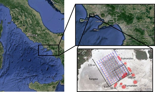
Satellite image of the Campi Flegrei region and zoom-in on the investigated area during the RICEN experiment, showing geometrical distribution of the sources (red circles) and receivers (blue triangles). The dimension of the subgrid used for the analysis is represented with the solid black square and the shifted overlapping subgrids are indicated with the dashed squares. The area for which the S-wave model is obtained is represented by the shaded grey box. In figure, Fangaia indicated the region at the boundary of the investigated area, where the water outcrops at the surface and the red points the fumaroles where high temperature is recorded.
A Geode G24 acquisition system was used, with a dynamic range of 24 bits, a full-scale voltage of 2.8 V and a sampling rate of 1 kHz. The trigger for the system was radio-controlled, to ensure correct timing for all of the sensors. When the Vibroseis was activated (i.e. lowered its mass to produce the energization), a radio signal was sent to the data logger, to open all of the recording channels. This guaranteed that the differences in the P-wave arrival times between close stations were due to the propagation of the seismic waves across the array. For each source position, three energizations were performed, and they were automatically stacked to increase the signal-to-noise ratio.
The Vibroseis produces vibrations in the frequency band of 5–125 Hz, with a 15-s-long linear sweep that is a signal where the dominant frequency increases linearly with time. Fig. 2 shows an example of the source signal recorded on the vibrating plate, and the associated spectrogram. It is worth noting that the spectrum of the source depended on the coupling of the mass with the ground, and it was usually not flat in the frequency range of 5–125 Hz. We observe that for frequencies >40 Hz, the source behaves as a high-pass filter with a flat level and a ratio of about 4:1 between the flat level and the amplitude of the spectrum, at 7 Hz.
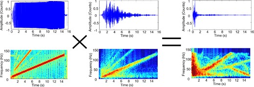
Examples of raw sweep data recorded during the experiment, with the results after the cross-correlation and the minimum phase filter, and their respective spectrograms. The first panel on the left shows the sweep function, the middle one displays the seismogram as recorded by the instrument and the right-hand panel shows the retrieved Green's function after correlation and filtering. All of the traces are normalized by their maximum. The panels on the right show that the largest part of the energy is concentrated in the first seconds of acquisition.
In this study, we investigate the shallow structure of the Solfatara using the surface waves as the diagnostic tool. In the next section, we discuss the data processing used to extract the Green's functions from the Vibroseis records. In the following section, we investigate the variability in the surface waves as a function of the frequency and the distance. After partitioning the investigated area into subgrids, we estimate the phase and group velocities using the coherence of the Rayleigh waves along the sections. We finally invert the dispersion curves to obtain a 3-D S-wave model for the area.
2 DATA PROCESSING
The filter parameters depend on the shape of the sweep, which results in a specific Klauder filter function (Brittle et al. 2001). Moreover, any autocorrelation function is a zero-phase filter, and its application to the Green's function yields a modification of the arrival times of the seismic waves, to produce a non-causal signal. To preserve causality in the data, an additional minimum phase filter is applied after cross-correlation (Gibson & Larner 1984).
Here, we therefore cross-correlate the data with the sweep source function, which were recorded on a specific channel of the acquisition system. An example of input and cross-correlated signals is shown in Fig. 2. Although the input sweep is expected to be the same for all of the vibrations, some differences arise from the different coupling of the Vibroseis plate with the soil. We checked the quality of all of the sweeps by comparison of the observed spectrograms with the expected spectrograms. In most cases, we get consistent source spectrograms. There are very few cases for which a different spectrogram is observed, due either to an error in the radio communication of the sweep or to bad coupling between the plate and the soil. In this case, we did not use the specific sweep function for cross-correlation, but we used the average of all of the consistent sweep functions.
We also checked the effect of the minimum phase filter on the data. We did not observe any significant changes after applying the minimum phase, neither in the first P-wave arrival time nor in the arrival time of the largest amplitude wave train. However, to preserve causality, we applied the minimum phase filter. Finally, each trace is normalized by the maximum of its absolute value.
3 PHASE AND GROUP VELOCITY ESTIMATION
For the estimation of the phase and group velocities associated with the Rayleigh waves, we want to use the coherence of surface wave propagation along seismic sections and the stack of the signals in the same distance range, to increase the signal-to-noise ratio and to reduce the small-scale variability that cannot be resolved by the data.
The coherence of the waveforms in the same distance range is enhanced for a 1-D horizontally layered structure and an isotropic source, with this latter condition almost satisfied by the Vibroseis. Under these assumptions, the signal is independent of the azimuth of the receiver and only changes as a function of the source–receiver distance, regardless of the absolute locations of both source and receiver.
Fig. 3 shows a seismic section associated with a single shot, where the data are filtered in the frequency band of 7–10 Hz. The largest amplitude in the data corresponds to the Rayleigh waves. Although we can follow the surface waves that propagate along the section at an almost constant velocity, there is also a general smearing of this wave packet, a transfer of energy from ballistic to coda waves as the distance increases, and a strong variability in the surface wave signals, as also for traces recorded at similar distances from the source. This variability indicates that a 1-D model does not provide a suitable description of the structure for interpretation of the surface wave propagation. Nevertheless, the coherence of the signal at short distances indicates that a 1-D model approximation holds locally, over a smaller space scale.
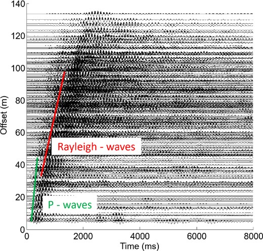
Filtered (7–10 Hz) seismic section of one shot recorded at all of the stations. The traces are ordered by distance from the source. The arrival times of the P waves and Rayleigh waves are indicated with two solid lines (green and red, respectively). Signals that deviate from these lines show the great spatial heterogeneity in the medium.
We then subdivide the receiver grid into smaller size subgrids, and determine whether there is any specific space length at which the signal remains coherent as a function of the distance. We thus recursively analyse squared overlapping subgrids, the sizes of which range from 20 m × 20 m up to 90 m × 90 m (the maximum allowed size for this experiment). We also subdivide the distance range into bins where we average all of the traces with sources and receivers in the same subgrid and the distance between them in the same bin, where the average is computed as the algebraic mean point-by-point along the trace. For each size, we investigate how coherent the signal remains along the section for several narrow frequency bands between 7 and 25 Hz. This lower limit is selected as the minimum frequency at which the energy radiated by the Vibroseis source can be clearly observed over the whole investigated area, regardless of the location of the source. This maximum frequency is chosen, instead, as the upper limit at which the energy coherently propagates across the Solfatara.
The maximum grid size at which the signal remains coherent along the section is 40 m × 40 m, as a subgrid that contains 9 × 5 receivers, and at a maximum of 5 × 4 shot locations. As we allow for the maximum overlap, the nearby grids are either shifted by 5 m along the in-line direction, or by 10 m along the cross-line direction, which leads to a total number of 96 subgrids. Within this partition, we obtain a coherent profile up to 20 m.
Finally, after selecting a subgrid partitioning of 40 m × 40 m, we also investigate the size of the bin according to which all of the source–receiver pairs that fall into the same distance range are stacked. This choice represents a compromise between a sufficient number of traces to be stacked to provide reliable averages, and the possibility to follow the surface wave features along the section with continuity. The best compromise is a binning of 1 m. An example related to one subgrid and containing the number of traces that are stacked in each bin is shown in Fig. 4. We have >10 traces to be stacked for most of the bins. The variability depends on the rectangular grid associated with the experiment.
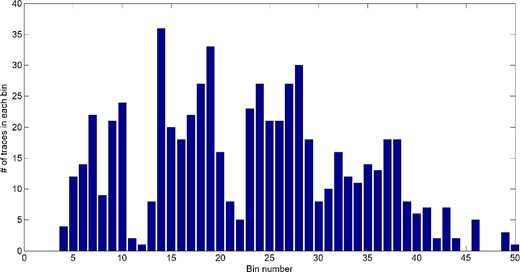
Number of source–receiver traces spatially averaged in each 1-m spatial bin for the subgrid used in Fig. 5. Due to the geometry of the experiment, we have not a uniform distribution of records with distance, but the selected sizes of subgrids and bins allow us to have a sufficient number of records for most of the bins.
Within this selection, we proceed to the estimation of phase and group velocities in each subgrid. For this goal, we filter the signal in 14 narrow overlapping bands between 7 and 25 Hz. We select the frequency bands using the criterion that the ratio between the width and the central frequency of the band is preserved. After filtering, we normalize each signal to its maximum.
To compute the phase velocity in a subgrid, we first gather the data into distance bins. An example of the resulting section is shown in Fig. 5(a), for the frequency band of 8.6–12.4 Hz, centred at 12 Hz. For the computation of the velocity, we perform a grid search with the velocity spanning the interval of 35–300 m s−1, with a step of 5 m s−1. For each velocity v, we shift back in time the traces of the value given by the ratio between the source–receiver distance and v. We then stack the moved out section up to 20 m. We expected that in agreement with the effective value of the velocity, the amplitude of the stack function would be large, because the waveforms along the section are almost in phase, while the amplitude of the stack is likely to decrease for velocities further and further from the effective velocity. Therefore, we use the maximum of the envelope of the stack signal as the fitness function. An example of this function is shown in Fig. 5(c), as associated with a section of Fig. 5(a). That function can have several local maxima, with oscillations for low velocities. Nevertheless, the absolute maximum is well resolved in almost all of the cases, although the quality degrades as the central frequency of the band increases.
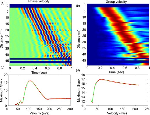
Filtered (8.6–12.4 Hz) average seismic section for sources and receivers selected in one squared subgrid (see Fig. 1). (a) Coherent average centred at 10.5 Hz, from which the phase velocity can be extracted. (b) Envelope of the coherent average from which the group velocity can be extracted. (c) and (d) Stack function for different velocity values used to realign the seismic sections in (a) and (b), and consequently to obtain the phase (c) and group (d) velocities. The blue lines in the panels (a) and (b) represent bins for which we have no records.
For the computation of the group velocity, we apply a similar technique, although we compute the envelope of the signals before building the binned seismic section for each subgrid. An example of this section is shown in Fig. 5(b). For computation of the velocity, we also perform a grid search, although we investigated a lower velocity range (20–210 m s−1, with a step of 5 m s−1). For each value, we align the traces, we compute the stack on the moveout section, and we use the maximum of the positive definite stack function as the fitness function. An example of the function is shown in Fig. 5(d), as associated with a section of Fig. 5(b). The absolute maximum of the function is smoother compared to the phase velocity. When increasing the frequency, bimodal or multimodal fitness functions occur for some subgrids, with comparable amplitudes of the maxima. In this case, we add a smoothness condition on the velocity as an additional constraint that penalizes significant jumps in the group velocity between consecutive frequency bands and contiguous subgrids in space. From this analysis, we get the dispersion curves in each subgrid. An example of this curve is shown in Fig. 6. As a general trend, the group velocity is always smaller than the phase velocity. While the phase velocity always decreases with frequency, the group velocity is almost constant, with local maxima and minima in several subgrids and different frequency bands.
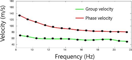
Representative data for phase and group velocity dispersion curves. On the horizontal axis, the central frequency for each band is reported. The curves generally show a decreasing trend with the frequency.
Fig. 7(a) shows the maps of the phase velocity for the different frequencies. They are plotted at different depths, because we use the implicit association that lower frequencies or longer wavelengths correspond to deeper regions. There are two anomalies at the boundaries of the investigated region. The NW anomaly also corresponds to the largest phase velocity measured in the area (250 m s−1), and it has a cross-line size of about 50 m, while it is thinner along the in-line direction. The SE anomaly has almost the same shape, although with smaller velocity values. The root of the NW anomaly can be seen in the whole frequency range, while the SE anomaly almost disappears at 17.5 Hz. Moreover, for frequencies >15 Hz, a faster velocity is observed in the SW part of the area, close to the Fangaia mud pool, compared to the NE domain. The retrieved velocities well superimpose on average to the values of the phase velocity, as obtained by Petrosino et al. (2012), in the overlapping frequency range (7–12 Hz), although the space scale at which they resolved the model is significantly larger than the space discretization used in this work.
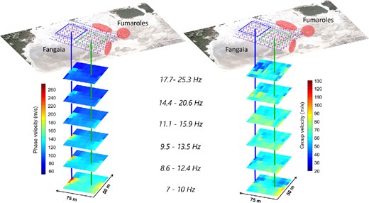
Spatial versus frequency representation of phase (a) and group (b) velocity maps. Different frequency bands classically investigate different depths for surface waves. Colour bars, variation of the phase and group velocities for the two different subgrids; blue and green squares at the surface, spatial extension of the subgrids; vertical lines (blue and green), centre of the two subgrids and associated to one pixel of the velocity maps. The overall map of the Solfatara is superimposed on the set of sources (red) and receivers (blue), where the location of the Fangaia and fumaroles (red points) is also indicated.
The group velocity in Fig. 7(b) also has a maximum at low frequency that corresponds with the SE anomaly retrieved for the phase velocity, although it shows a minimum for the NW anomaly. These features do not have roots as deep as for the phase velocity. At higher frequencies, the main peculiarity is the separation between the SW domain, which is slightly faster than the NE region, as also observed for the phase velocity. Finally, in the last frequency band (17.7–25.3 Hz, centred at 21.5 Hz), very small velocities (i.e. ∼30 m s−1) are obtained corresponding to the NW anomaly.
4 S-WAVE VELOCITY MODEL FROM INVERSION OF THE DISPERSION CURVES
The phase and group velocity dispersion curves were jointly inverted to determine a velocity model of the whole area. We first inverted the dispersion curves in each subgrid, to compute a 1-D velocity model local to the subgrid. Then the combination of the models for all of the subgrids provides us with a 3-D model. For the inversion, we use the Geopsy software (Wathelet et al.2004), which searches for the best horizontally layered P-wave and S-wave models that fit the dispersion curves. To retrieve the velocity structure, the number of layers, the range of variability for the P-wave and S-wave speeds and the density are required. We first observe that the results are relatively insensitive to the P-wave model and the density. Hence, we limit the exploration to the S-wave velocities and to the depth of the interfaces.
We perform several tests to correctly set the number of layers and the maximum penetration depth of the Rayleigh waves. We consider a four-layered model as the best choice, because the misfit between the simulated and expected dispersion curves significantly reduces up to four layers, while there is no further large reduction when the number of layers is increased beyond this value. The range for the S-wave speed was selected as between 50 and 1250 m s−1 (Letort et al.2012).
An example of the S-wave models obtained from inversion of the dispersion curves is shown in Fig. 8. From Fig. 8, we see that several models provide very similar fits for the dispersion curves. A four-layer model still provides a smooth dispersion curve that cannot match all of the slope breaks that we can observe in the real dispersion curves. This is the case of the dispersion curves plotted as solid black lines in the upper part of Fig. 8, which correspond to the largest phase-velocity region. When the dispersion curve is smoother, this is well retrieved by the model, as for the example shown in the bottom part of Fig. 8. This latter region is related to a subgrid in which a low phase velocity is measured. For the sake of completeness, the dispersion curves for the phase and group velocities, with the misfit, are also shown. As a general comment, the first very shallow layer is always well constrained and reaches a maximum depth of 4 m. A second layer has depths between 4 and 8 m. Finally, the depth of the last interface and the velocity below it are not well constrained. This layer could be the interface between the unconsolidated shallow deposits and the aquifer beneath the Solfatara that clearly emerges in the Fangaia mud pool. Although the study of Petrosino et al. (2012) was based on a larger space scale, lower frequency range and consequently larger penetration depth, the interface that they retrieved at about 5 m well corresponds on average to the variation of S-wave velocity in the first two layers of the model obtained in this work.
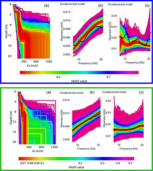
(a) Representations of the inverted layered model for the two subgrids indicated by the same colours in Fig. 7 (blue, top panel and green, green panel). (b) Phase velocity. (c) Group velocity. Black lines, experimental dispersion curves; coloured curves, numerical dispersion curves for a wide distribution of layered models.
From the analysis, we did not select the single best-fit model, but we decided to extract all of the profiles from the exploration ensemble with misfit <15 per cent, compared to the minimum value. We assume as best model the average of the selected models. The average models are no longer layered; they are instead characterized by the almost continuous variation of the wave velocity with depth. We finally combine the 96 velocity profiles to retrieve lateral 3-D variations in the S-wave velocity within the medium.
Fig. 9 (right-hand panel) shows the velocity model for fixed depths, from 4 to 12 m below the Solfatara surface (at an altitude of 97 m) with a step of 2 m. This model is compared with the resistivity model obtained on the same area (see below). We do not represent the velocity model above 4 m because with this range of velocities (100–600 m s−1), we do not have a good resolution of the lateral variation.
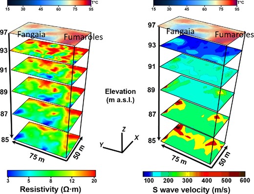
Spatial versus depth representation of S-wave velocity map (right) and comparison with geoelectric resistivity measurements (left) on the same spatial grid. The altitude of the Solfatara area is 97 m and the depth is plotted downwards from this reference. The temperature map with the position of mud pool and fumorales is shown at the top.
We note that the two NW and SE anomalies observed in the phase-velocity maps, clearly appear as high-velocity bodies at all depths. Specifically, the NW anomaly is a clear spot that emerges at 4 m and becomes more evident in terms of the velocity contrast at greater depths. The SE anomaly appears at 8 m and preserves its shape with increasing depth. We also note that the SW domain is slower at all depths, compared to the NE domain. This area is the side closest to the Fangaia, where the water outcrops, and it might be the manifestation of an unconsolidated layer at shallow depths and of a water aquifer at greater depths. This statement is confirmed by Fig. 10, where we plot different isosurfaces of velocity (100, 150, 200 and 300 m s−1) and an isosurface of resistivity at 8.5 Ω⋅m. The isoresistivity surface shows low-level resistivity near the Fangaia, which therefore indicates a soil rich in water. Indeed, at the same time, the isovelocity surfaces show a clear decreasing gradient toward the Fangaia side. As the resistivity curve goes down following the aquifer, the shear wave velocity decreases close to the surface, due to the presence of water. Fig. 10 is obtained using the same data as in Fig. 9, with a spatial filter that smooths the short-range velocity contrast. This filter allows us to focus on the average trend observed with the velocity gradient at lower frequencies toward the Fangaia mud pool.
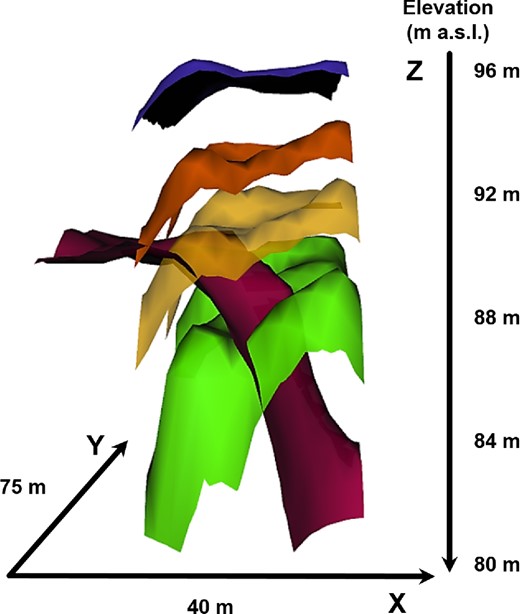
Representation of the isovelocity surfaces for velocities of 100 m s−1 (blue), 150 m s−1 (orange), 200 m s−1 (yellow) and 300 m s−1 (green). Purple surface, isoresistivity at 8.5 Ω⋅m. The same low-order spatial filter was applied to smooth the short-scale spatial heterogeneities (see Fig. 9) and to reveal any global trend of the shear velocity and resistivity gradients. This figure has the same orientation of Fig. 9.
5 DISCUSSION
The goal of the RICEN experiment at Solfatara is to determine whether combined active and passive seismic measurements can be used to accurately characterize the structure of an active hydrothermal area and its changes with time. This first study is aimed at defining the very shallow structure of the area, down to 12–15 m, using Rayleigh waves. These data are complementary to velocity models obtained from the inversion of P-wave traveltimes, which explore greater depths. The P waves generated by active experiments in the area (Bruno et al.2007; Festa et al.2015) cannot define the features of this very shallow region, because body-wave rays have an almost vertical incidence below the stations, due to the strong velocity gradient. The time delay is indeed integrated over the first 10–15 m beneath the station, independent of the source position, and it eventually appears as a residual contribution in the traveltime difference between synthetics and observations. Moreover, the measure of the P wave at very short source–station distances (<10 m) is not accurate, because the minimum wavelength in the source time function is comparable with such a distance. On the contrary, the surface waves can correctly explore the features of this shallow region. Due to the strong velocity gradient, the low-frequency (7–25 Hz) Rayleigh waves are trapped in this very shallow domain beneath the Solfatara. Additionally, the criss-crossing of the seismic rays from the large number of stations and the source position increases the horizontal resolution in the models.
To have a complete description of the investigated area, seismic models are compared to the results from the electrical resistivity tomography, which has good resolution in the discrimination of media that are rich or poor in water and gas. The electrical resistivity tomography is obtained performing direct-current resistivity profiles, with sixteen 115-m-long profiles with NW–SE orientation and twenty-four 75-m-long orthogonal NE–SW profiles, all with 5 m spacing between the electrodes. The same Wenner–Schlumberger configuration is used for all of the profiles, and the 3-D inversion is obtained using an algorithm as detailed by Loke & Barker (1996) and implemented in the RES3DINV software (Loke & Dahlin 2002). The normalized root mean square error of the resulting 3-D model is 7.5 per cent, and the data quality allows for a high-resolution resistivity model down to 15 m in depth. Also, acquisition of the soil temperature at 30 cm in depth is performed at each electrode during the experiment. Resistivity maps are represented on the left side of Fig. 9, at the same depths as the S-wave velocity maps. The temperature field is added on the top of the resistivity and seismic profiles.
In the temperature field, there is a cold region at about 50–60 °C in the central part of the area, beside the Fangaia, which is surrounded by a hot domain with spots that reach 90–95 °C, where the fumaroles emerge at the surface. The resistivity model in the first 4 m is correlated with the temperature field, with resistive bodies that correspond to high-temperature regions. Hence, high-temperature regions/high resistive bodies are likely to be related to the presence of rock filled with high-temperature gases. These regions also correspond to low-velocity domains very close to the surface in the seismic model, although there is no clear correlation between the S-wave model at 4 m with the temperature field, as can be seen in the resistivity map at the same depth. Nevertheless, shallow velocity anomalies are mostly related to the temperature gradient. Hence, a change in the temperature can be associated with a rheological/ lithological transition between rocks with different properties, such as with different degrees of water or vapor saturation. Between 8 and 10 m in depth, there are two strong anomalies at the boundary of the model, with an increase in the S-wave velocity by a factor of 2–3. These two anomalies also appear in the resistivity maps as a transition between an upper resistive, probably gas-rich, domain to a less resistive region, which appears to be representative of rock with significantly lower gas content. At greater depths, this anomaly appears to extend over a broader region, although it is probably a smearing effect due to loss of resolution as the investigation depth increases. Finally, at 12 m in depth, we observe a separation of the SW domain from the NE domain, with the NE domain significantly faster in terms of S-wave velocity. This boundary clearly appears in the resistivity profile as a transition to a conductive region (5 Ω⋅m) close to the Fangaia mud pool, which is interpreted as a water-saturated layer (Byrdina et al.2014). As the water emerges at the Fangaia, we expect that the water layer at depths of 10–12 m in the SW domain of the investigated area stops or sharply deepens when moving towards the NE. This is also observed clearly by the isosurfaces of the velocity and resistivity that show a complementary trend; in the area where there is low resistivity, the S waves are slower than where there is high resistivity.
6 CONCLUSIONS
In this study, we analysed active data recorded during the first stage of the RICEN experiment at the Solfatara, Campi Flegrei, Italy. After processing the data to remove the source time function of the Vibroseis, we investigated the Rayleigh wave dispersion in terms of both phase and group velocities in the frequency range 7–25 Hz. To have a robust estimate of the wave speed as a function of the frequency, we first investigate the maximum size for which the assumption of a 1-D velocity structure with depth is reliable. A 1-D approximation holds up to distances of 40 m within the investigated area. Then, we subdivide the area in squared subgrids with sides of 40 m, and within each subgrid we stack all the signals in the same source–receiver distance, independent of the absolute positions of the sources and stations. We estimate the phase and group velocities for each subgrid, to search for the maximum of the stack function after aligning the traces for the selected velocity. The stack is computed on the traces for the phase velocity and on the envelope of the traces for the group velocity. Finally, the phase and group velocities are jointly inverted to provide a 3-D S-wave model for the Solfatara area. We find that the maximum penetration depth is 12–15 m for the selected frequency range. At shallow depths, there are velocity anomalies that are correlated with the temperature gradient measured close to the surface, while at greater depths the anomalies correspond to transition between a gas-rich region to a water-saturated layer, which is outcropping SW outside of the analysed domain.
We acknowledge Marc Wathelet for his help in the use of the Geopsy software, and for providing us with scripts for the analysis of Geopsy outputs. ISTerre is part of Labex OSUG@2020. This study was carried out within the framework of the MedSuv project, which received funding from the European Union Seventh Programme for research, technological development and demonstration, under grant agreement no.308665.
We are grateful to two anonymous reviewers that contributed in improving the manuscript.
REFERENCES
