


Abstract
We review the theory of the Earth's elastic and gravitational response to a surface disk load. The solutions for displacement of the surface and the geoid are developed using expansions of Legendre polynomials, their derivatives and the load Love numbers. We provide a matlab function called diskload that computes the solutions for both uncompensated and compensated disk loads. In order to numerically implement the Legendre expansions, it is necessary to choose a harmonic degree, nmax, at which to truncate the series used to construct the solutions. We present a rule of thumb (ROT) for choosing an appropriate value of nmax, describe the consequences of truncating the expansions prematurely and provide a means to judiciously violate the ROT when that becomes a practical necessity.
1 INTRODUCTION
The problem of computing the deformations of an elastic body subject to surface loads has a very long history involving many illustrious mathematicians and physicists (Boussinesq 1885; Lamb 1901; Love 1911, 1929; Shida 1912; Terazawa 1916; Munk & MacDonald 1960; Longman 1962, 1963; Farrell 1972). The easily-coded solution for a uniform elastic half-space (Becker & Bevis 2004) is useful in many engineering contexts, but it is often inappropriate for geophysical applications, since the Earth is neither a half-space nor homogeneous. The solution for a layered elastic half-space (e.g. Pan et al.2007) has wider applicability, but even this formalism is inappropriate for loads with large apertures, or to compute deformations at large distances from the load, where large refers to a significant fraction of the Earth's radius, or greater. Therefore, the preferred framework for most geophysical applications is that of a layered, elastic, self-gravitating sphere with a fluid core (Farrell 1972). The solution for this problem is nearly always developed in terms of expansions involving the load Love numbers, often represented using the symbols (|$h^\prime _n, k^\prime _n, l^\prime _n$|), or just (hn, kn, ln) when the loading context is clear. Typically, these treatments invoke either point loads or disk loads.
The point load formalism is often invalid close to the nominal point load, and in that sense the disk load formalism is more flexible. We note that the Love number formalism is appropriate for spherically symmetric elastic Earth models; transverse anisotropy can be incorporated in this class of models as long as it honours spherical symmetry (Pan et al.2015). General classes of elastic anisotropy (e.g. laterally varying transverse and azimuthal anisotropy) break spherical symmetry, in which case the Love number approach is no longer appropriate, and different approaches such as self-gravitating finite element models are needed (though they present their own computational difficulties). Anyone using the equations and the code presented in this paper is implicitly assuming that elastic anisotropy is either absent or of a very special kind.
Between 1975 and 2000, most of the geophysical literature on the surface loading problem focused on glacial isostatic adjustment which addresses the loading response of a viscoelastic Earth (Haskell 1935; Cathles 1975; Peltier & Andrews 1976; Wu & Peltier 1982). Nearly all of these studies also use a Love number formulation. The linear elastic and linear viscoelastic versions of the loading problem are connected via the elastic-viscoelastic correspondence principle (Alfrey 1944; Read 1950; Lee 1950). But, beginning in 2001, there has been a major resurgence of interest in the purely elastic problem. This is because (i) geodesists and geophysicists began to realize that networks of Global Positioning System (GPS) receivers, and more recently Global Navigation Satellite System (GNSS) receivers, were recording seasonal, sustained (i.e. progressive) and transient elastic displacements driven by contemporary changes in the loads imposed on the solid Earth by water, snow and ice (Blewitt et al.2001; Heki 2001; Mangiarotti et al.2001; Dong et al.2002; Bevis et al.2005) and, to a lesser extent, by atmospheric pressure variations (Vandam et al.1994), and (ii) geodetic observations of the Earth's elastic deformation could be used to monitor changes in ice mass (Khan et al.2010; Bevis et al.2012; Nielsen et al.2012; Spada et al.2012; Nielsen et al.2013) and in terrestrial water storage (Bevis et al.2004, 2005; Steckler et al.2010; Fu et al.2013; Borsa et al.2014), and so provide a new means to study climate cycles and climate change.
The easiest way to characterize a distributed load or load change is to represent it as one or more, often many more disk loads. If mass or mass change fields are represented as grids, then each grid cell can be treated as a disk load or, should it reside in the far-field of the geodetic station, as a point load. The response to a point load can be equated with that of a small and remote disk load, except very close to the point load where the point load concept itself is almost never realistic. Our purposes in this paper are two-fold. First, we wish to provide non-specialists with a simple but complete discussion of how to compute the Earth's elastic response to a disk load. We provide a matlab function (diskload) that implements this algorithm. Our code, like nearly all of its cousins, sums terms consisting of load Love numbers and Legendre polynomials, or derivatives of Legendre polynomials, all of degree n = 0, 1, 2, …nmax. It is important to choose an appropriate value for nmax, especially when we seek accurate estimates of the near-field response to the load. Second, we explain how do this, and examine the consequences of prematurely truncating the expansion, that is, choosing or setting nmax too low. This mistake is quite easily made when modelling the elastic response of geodetic stations located close to the edge of ice sheets whose mass losses are being characterized with very high resolution digital elevation models (DEMs), since the appropriate value for nmax increases inversely with the grid spacing or cell size of the DEM. We hope that this discussion will help our readers use more general and complex software packages, such as REAR (Melini et al.2015a,b) with increased confidence.
2 THEORY
The so-called ‘disk load’ is a particular type of surface mass density distribution, characterized by a (i) uniform imposed pressure, that is, constant load ‘thickness’, and (ii) axial symmetry, two features that make the disk load very handy in applications related to glacial isostasy (e.g. Spada et al.2012; Melini et al.2015b) because of its straightforward expansion in a series of spherical harmonic functions. The disk load can be defined in several ways, which differ in how the problem of mass conservation is addressed (Spada 1993).
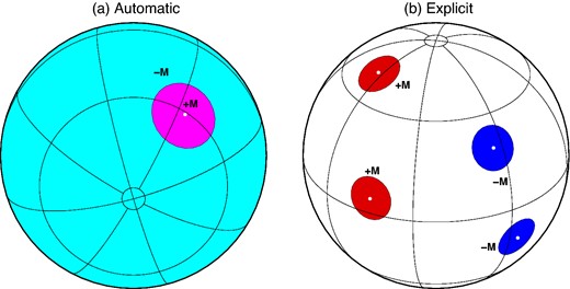
Two ways of conserving the total mass of the load. In panel (a), the disk load of mass +M = Mdisk (magenta) is automatically compensated by a complementary load of mass −M (cyan) according to eq. (4). In panel (b), several disk loads like (1) are explicitly used (red) and compensated by disks of mass −M (blue), with a vanishing total mass. Small white circles mark the poles of the disk loads.
Alternatively, if one invokes an uncompensated disk load, mass can be still be conserved by introducing one or more additional uncompensated disk loads such that their total mass is zero. This approach is illustrated in Fig. 1(b). In this case mass conservation is accomplished on the basis of some specific geophysical intuition. For example, if the primary disk load represents an ice cap, the compensating ones could be distributed over the oceans to fit the shape of the coastlines. The number of free parameters would increase, but this will be accompanied by an increased accuracy of the global load (note that such a distribution of disks would, unavoidably, contain interstices or overlaps). Again, exploiting the symmetry of each individual disk load and using the superposition principle, the problem can be reduced to the computation of the Earth's response to one single uncompensated disk load, which enormously facilitates the numerical applications (e.g. Spada et al.2012; Melini et al.2015b).
The formulae presented above are implemented in our matlab function diskload (see Supporting Information Text S1).
3 THE LOAD LOVE NUMBERS
The load Love numbers (hn, kn, ln) depend on the elastic structure of the Earth, so each Earth model is associated with its own set of Love numbers. Computing the Love numbers is considerably more difficult than using them to compute the elastic response to a disk load, and as a result this task is usually left to specialists (see e.g. Pan et al. 2015 and references therein). In addition to our matlab function diskload, we provide the reader with a set of Love numbers associated with the seismological Earth model REF of Kustowski et al. (2007). This set of Love numbers, which we use in Section 4, is complete through degree 40 000. Obviously, utilizing this particular set of Love numbers with diskload means we can invoke nmax ≤ 40 000, but no higher. However, users of diskload can use Love numbers associated with other Earth models, and seek out Love number listings that permit higher values of nmax. According to our experience, standard Fortran routines (e.g. Press 2007) and the matlab function pLegendre that comes with diskload can compute reliably the Legendre polynomials to harmonic degrees as high as 107. However, possible errors can be associated with the evaluation of high degree Love numbers, unless the computations are performed with sufficient precision (Spada 2008; Spada et al.2011) and possibly with the help of analytical solutions (Grapenthin 2014; Pan et al.2015).
In Fig. 2, the Love numbers for the seismological model REF of Kustowski et al. (2007) are shown as a function of the harmonic degree n. The Love numbers are expressed in the reference frame having the origin in the centre of mass of the (Earth+Load) system, which imposes 1 + k1 = 0 (Farrell 1972). With a different choice of the reference frame, the value of the three degree n = 1 Love numbers would be modified (Spada et al.2011). While the Love number for vertical displacement (hn) reaches a constant value with increasing n, those for horizontal displacement (ln) and for the gravitational potential (kn) decay as |${1}/{n}$|. As pointed out by Farrell (1972), the asymptotic dependence of the Love numbers for large n values matches the solution of the Boussinesq problem, which applies to a flat and homogeneous Earth model (Boussinesq 1885). This shows that with increasing n the Love numbers become increasingly sensitive to the values of the elastic constants of the Earth's outmost layers. This property can be exploited to test the consistency of numerical computation of high-degree Love numbers (Farrell 1972) or to approximately extend a given set of Love numbers to higher harmonic degrees.
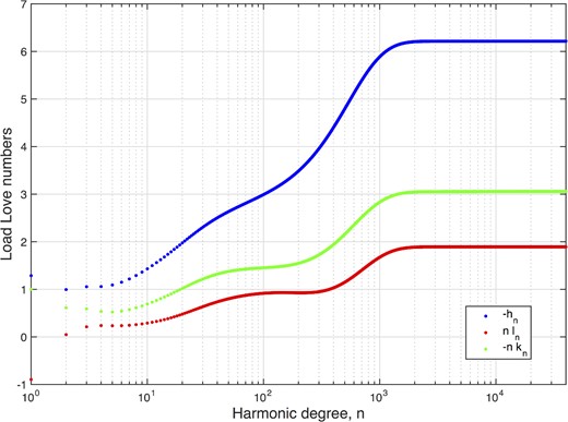
Load Love numbers (hn, kn, ln) for model REF, as a function of harmonic degree n. Note that h0 = −0.216 and k0 = l0 = 0 are not shown due to the logarithmic scale.
4 THE TRUNCATION PROBLEM
We now illustrate the issues pertaining to the ROT using the case of a compensated ice disk load with angular radius α = 0.1° and a thickness of T = +1 m. Our ROT requires us to set |$n_{{\rm max}} \gtrsim \overline{n}_{{\rm max}}$| and since |$\overline{n}_{{\rm max}} = 3600$|, for a disk of radius 0.1°, this requirement is easily satisfied if we set nmax = 40 000. Accordingly, we used diskload, with nmax set to 40 000, to compute the vertical U(ϑ) and horizontal V(ϑ) components of displacement as functions of the angular distance, ϑ, measured from the centre of the disk. We can think of ϑ as colatitude referred to a pole in the centre of the disk. In Fig. 3, we graph U, V and G as functions of the normalized distance ϑ/α, emphasizing the near-field (Fig. 3a) and the far-field (Fig. 3b) responses. We note that effectively the curves always depend on ϑ and α, not ϑ/α, and there is no ‘universal’ shape to the curves no matter how the plot axes are normalized (see Supporting Information Text S3). The curves in Fig. 3 reproduce, to very high precision, those computed by the program REAR (Melini et al.2015a), thereby validating our matlab function. Note that the load causes elastic subsidence (U(ϑ) < 0) which attains its extreme value (−2.09 mm) at the centre or pole of the disk, and poleward horizontal displacement (V(ϑ) < 0) which attains its extreme value (−0.33 mm) at the edge of the disk. The amplitude of V(ϑ) falls to zero at the centre of the disk, as required by the axial symmetry of the load. The amplitudes of both components decrease monotonically with increasing distance from the edge of the load. The geoid height variation G(ϑ) attains positive values, which denotes an under-compensated load (Spada et al.2011), and it is strongly anti-correlated with U(ϑ). At the pole of the load, its maximum amplitude is +0.43 mm. Maximum values of U, V and G are found to depend linearly on the disk size for small loads, matching the scaling laws that hold for the flat and homogeneous Earth model (see Supporting Information Text S3; Boussinesq 1885; Lamb 1901; Terazawa 1916).
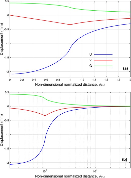
Vertical displacement (U), horizontal displacement (V) and geoid height variation (G) for an ice disk load with α = 0.1° and thickness T = +1 m, as a function of ϑ/α, in the near field (a) and in the far field (b). Disk thickness is expressed as equivalent water height corresponding to an ice density ρi = 917 kg m−3.
We now consider, in Fig. 4, what happens when we set |$n_{{\rm max}} \approx \overline{n}_{{\rm max}}$| or if we truncate the expansions prematurely by setting either |$n_{{\rm max}} < \overline{n}_{{\rm max}}$| or |$n_{{\rm max}} \ll \overline{n}_{{\rm max}}$|. We define the numerical maturity of our expansions, M, to be |$n_{{\rm max}}/\overline{n}_{{\rm max}}$|. For all practical purposes, the solution obtained with nmax = 40 000 can be considered, for α = 0.1°, the true solution. From the results in Fig. 4, it is apparent that for |${n}_{{\rm max}}=\overline{n}_{{\rm max}}=3600$| (light green curves) the ‘true’ solutions obtained using nmax = 40 000 (see dashed lines) are reasonably well reproduced. However, oscillations due to the deficiency of short-wavelength terms imposed by premature truncation of the Legendre expansions (10) and (12) are clearly visible in the whole range of ϑ values. Note that the extreme values U(ϑ = 0) and V(ϑ = α) are approximated well and fairly well, respectively. A value |$n_{{\rm max}}=2 \, \overline{n}_{{\rm max}}= 7200$| (red curves) would basically reproduce the true solutions (this would suggest, for the ROT, the more conservative but more time consuming choice |$\overline{n}_{{\rm max}}=7200$|). Overall, the displacements obtained using |$n_{{\rm max}}=\overline{n}_{{\rm max}}/2 = 1800$| still bear a marked resemblance to the true displacements; however, decreasing nmax below this value produces a complete deterioration of the solutions.
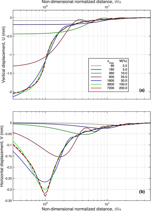
Surface displacements U(ϑ) (a) and V(ϑ) (b), obtained adopting a range of truncation degrees nmax, varying from |$n_{{\rm max}}=2 \, \overline{n}_{{\rm max}}$| (where |$\overline{n}_{{\rm max}}=3600$| corresponds to the ROT given by eq. 14) down to nmax = 90. Here M represents the ratio |$n_{{\rm max}}/\overline{n}_{{\rm max}}$|, expressed as a percentage. The dashed curve, reproduced from Fig. 3, is for nmax = 40 000.
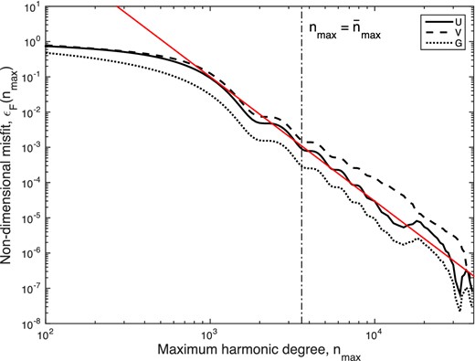
Misfit value |${\cal E}_F$|, defined by eq. (16), as a function of the truncation degree nmax, for F(ϑ) = U(ϑ), V(ϑ) and G(ϑ) (see solid, dashed and dotted curves, respectively). The vertical segment shows the |$\overline{n}_{{\rm max}}$| value. The red line shows the best-fitting linear relationship (16).
5 CONCLUSIONS
We have shown that one can normally compute the geoelastic response to a disk load with acceptable accuracy by setting the spectral truncation degree |$n_{{\rm max}} = \overline{n}_{{\rm max}}$|, as defined in the eq. (14), which constitutes our ROT. In the event that the station of interest is located right at the edge of the disk, and one is particularly interested in the vertical component of displacement, it would be reasonable to set |$n_{{\rm max}} = 2 \, \overline{n}_{{\rm max}}$| instead. However, while |$\overline{n}_{{\rm max}} = 3600$| for a disk with a 0.1° radius, |$\overline{n}_{{\rm max}}$| raises to 36 000 or 360 000 if the disk radius is reduced to 0.01° or 0.001°, something that is becoming a practical possibility given the increasing availability of ultra-high-resolution DEMs for the Antarctic and Greenland ice sheets and for many smaller ice fields and ice caps in other parts of the world. Computing the geoelastic response with very large values for nmax naturally rises concern because (i) the analyst may not be able to find lists of Love numbers that extend to very high degrees, and (ii) even if he or she could, there is some anxiety about how numerical round-off might have affected the computation of these Love numbers and/or any computations that utilize them. Since the amplitudes of the errors associated with premature truncation diminish quite rapidly with increasing distance from the disk, and because we normally model a distributed load (or load change) with a great many disks, very few of which have any stations in their near-field or even medium-field, the idea of judiciously and safely violating the ROT (14) becomes increasingly attractive. The best approach for doing this is to compute the total elastic response at each station due to all disks using multiple values for nmax, so that the sensitivity to nmax can be carefully assessed. As we explain in the Supporting Information annex, our function diskload provides an efficient mechanism for doing this.
The figures have been drawn using the Generic Mapping Tools (GMT) of Wessel & Smith (1998). MB was supported by National Science Foundation (NSF) grant ARC-1111882. GS is funded by Programma Nazionale di Ricerche in Antartide (PNRA) 2013/B2.06 (CUP D32I14000230005). We thank Gaia Galassi for discussion and Pascal Gegout for providing the load Love numbers for the seismological model REF of Kustowski et al. (2007).
REFERENCES
SUPPORTING INFORMATION
Additional Supporting Information may be found in the online version of this paper:
Figure S1. Vertical (U), horizontal (V) displacement and geoid change (G) for a disk load with α = 0.1° and load thickness Tw = +1 m, as a function of normalized colatitude ϑ/α, computed with nmin = 0 and nmax = 40 000.
Figure S2. Vertical (U), horizontal (V) displacement and geoid change (G) for a disk load with α = 0.1° and load thickness Tw = +1 m, computed at a colatitude ϑ = 1.5 α as a function of the maximum degree nmax. The U component oscillates to larger nmax than V and G since hn reaches a constant amplitude with increasing n while ln and kn decay as n-1, thus stabilizing faster (see main text). Horizontal dashed lines represent the ‘true’ values computed at nmax = 40 000; vertical dash-dotted lines mark the ‘rule of thumb’ |$\bar{n}_{{\rm max}}$| = 3 600, and the ‘safer rule of thumb’ |$\bar{n}_{{\rm max}}$| = 7 200, according to eq. (14).
Figure S3. Non-dimensional misfit εU as a function of disk radius α and truncation point nmax (blue contours) and its linear regression model according to eq. (S1) (red contours). The green dashed line represents the ‘rule of thumb’ |$\bar{n}_{\rm max}$| = 360°/α.
Figure S4. 3D view of the non-dimensional misfit εU as a function of disk radius α and truncation point nmax. The wire-frame plane represents the error regression model of eq. (S1).
Figure S5. Misfit value εF as a function of the truncation degree nmax for various disk sizes α. The vertical segments mark the |$\bar{n}_{{ max}}$| value defined in eq. (14); the red line corresponds to the global approximation presented in eq. (S1).
Figure S6. (a) Normalized surface displacements for various values of α, (b) Maximum values of surface displacements with varying α. Dashed lines show a linear scaling. In both frames, Tw = +1 m.
Table S1. Contents of the diskload.zip archive.
Please note: Oxford University Press is not responsible for the content or functionality of any supporting materials supplied by the authors. Any queries (other than missing material) should be directed to the corresponding author for the paper.
