Fast determination of earthquake magnitude and fault extent from real-time P-wave recordings

Abstract

INTRODUCTION

The increasing demand for prompt information shortly after a seismic event, has favored the development and diffusion of Earthquake Early Warning Systems (EEWS) in many countries worldwide. Operational EEW platforms are already available in Japan, Mexico, Romania, Turkey and Taiwan, while EEWS are under development or testing in California, Southern Italy, China, Iberian Peninsula and South Korea. EEWS are real-time, seismic monitoring systems, able to detect an ongoing earthquake and provide a warning to a target area, before the arrival of the most damaging waves. As soon as a seismic event is identified by one or more stations, the EEW platform rapidly estimates the main source parameters (event location and magnitude) within a few seconds from the earthquake occurrence. Location and magnitude are then used to provide a warning to a distant target area, where the strongest shaking is expected to occur, for the immediate activation of emergency procedures.

The source characterization in EEWS is usually based on the measurement of a peak amplitude or a characteristic period in the early portion of the recorded P and S wave train (typically 3–4 s). These parameters are related to the earthquake size or to the peak ground shaking (peak ground velocity, PGV and peak ground acceleration, PGA) through empirical relationships (Allen & Kanamori 2003; Kanamori 2005; Wu & Zhao 2006; Zollo et al.2006; Böse et al.2007; Wu & Kanamori 2008; Zollo et al.2010). Among the different parameters, Zollo et al. (2006) showed that the Peak Displacement amplitude of high-pass filtered P-wave signals (P_d) is correlated to the earthquake magnitude and distance, through a typical attenuation relationship. P_d is measured on the vertical component of the displacement waveforms in a 2–4-s time window after the arrival of the first P wave and is used to get a rapid estimate of the event magnitude, given a preliminary constraint on its location.

The use of limited P wave signal portions for the magnitude estimate is an implicit assumption of a point-source model for the earthquake rupture, for which most of slip is confined in a small region around the earthquake nucleation zone and is released within a short time interval. While these assumptions are generally acceptable for small-to-moderate events, they may not be appropriate when an earthquake rupture extends over few tens to several hundreds of kilometres on the fault (M ≥ 7–7.5), and the slip release may occur at large asperities located far away from the hypocentre. The most critical consequence of these assumptions is that the empirical regression relationships between EW parameters and magnitude, which are calibrated on short portion of P-wave signals, saturate beyond a magnitude 6.5–7, with consequent underestimation of the event size and significant biases in the prediction of the ground motion for large earthquakes (Kanamori 2005; Rydelek & Horiuchi 2006; Rydelek et al.2007; Zollo et al.2007; Festa et al.2008).

With the aim of improving the accuracy of source parameter estimation in real-time, new strategies for EEW have been recently proposed, mostly based on the rapid inversion of geodetic and/or accelerometer data, to estimate the rupture area extent and the slip distribution on the fault (Allen & Ziv 2011; Ohta et al.2012; Colombelli et al.2013; Wang et al.2013; Zhang et al.2014). Using strong motion data, Colombelli et al. (2012), suggested that the real-time parameter measurements are done in progressively expanded P-wave time windows (PTWs). They showed, indeed, that the standard methodologies and the existing empirical regression relationships can be extended to very large earthquakes, provided that appropriate time windows are selected for the parameter measurement.

The present work is intended to be a new contribution to the rapid characterization of the extended source. We propose here a straightforward methodology, solely based on the P wave vertical amplitude of the recorded seismograms, to quickly characterize both the magnitude and the finite extent of the seismic source. While the proposed methodology is aimed at the use in real-time and near-real-time applications, we focus here on the theoretical aspects of the methodology rather than on the practical implementation of the real-time algorithm.

METHOD

The present analysis is based on the results of Colombelli et al. (2014), which we briefly recall here for clarity. Using a database of Japanese events, Colombelli et al. (2014) looked at the time evolution of the logarithm of the peak displacement as a function of the P wave time window (hereinafter LPDT curve). The database they used consisted of 43 moderate-to-strong events (magnitude range 4 ≤ M ≤ 9) and 7514 waveforms, recorded at a maximum distance of 500 km (Text S1 and Fig. S1). Displacement waveforms are obtained after double integrating and high-pass filtering the acceleration records. For each record, the peak displacement amplitude on the filtered P wave signals (P_d) is measured over a progressively expanded PTW, starting at the P wave onset time and terminating at the expected arrival of the S waves (Fig. 1a). For each event, the LPDT curve is obtained by averaging all the available data in each time window, after correcting the observed P_d values for the attenuation effect (Text S2 in the Supplementary Material). An example of LPDT curve for a single event is shown in Fig. 1(b). For all the analysed events, the LPDT curves start with small values and progressively increase with time, until a plateau value is reached. Such a shape is common for all events in the whole explored magnitude range and generally, the greater is the magnitude, the larger is the plateau level and the longer is the time needed to reach it. Each LPDT curve is modelled using a piecewise, linear function, consisting in two, positively sloping straight lines and a flat plateau level (Fig. S2). Five parameters are estimated by fitting the curves with this model: the corner time of the first and second straight line, the slope of the two lines, and the final plateau level. A clear correlation with magnitude was found for all the fitting parameters, except for the second slope, for which no evident correlation with magnitude appeared. In their previous work, Colombelli et al. (2014), mostly focused on modelling the initial part of the LPDT curves for its possible relation with the beginning of the rupture process. We focus here on the final part of the curves and on its potential to provide insights on the source extent. The Plateau level (PL) and the corresponding time (T_PL) are empirically related to the earthquake magnitude, as shown in Figs 1(c) and (d). Here we investigate whether and how PL and T_PL can provide a rapid estimate of the event magnitude and of the expected length of the rupture.

Figure 1.

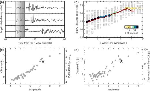
Parameters and method. (a) Example of displacement waveforms, arranged as a function of distance, from top to bottom, and aligned to the first P wave arrival time (thin, solid grey line). The shaded box shows the concept of expanding PTWs (dashed grey lines), starting at the P wave arrival time and terminating at the S wave arrival time (thick, black marker on each waveform). For each event, the LPDT curve is obtained by averaging all the available data in each time window, after correcting the observed P_d values at for the attenuation effect. (b) Example of LPDT curve for the 2000, Tottori earthquake. The coloured circles represent the value of the average LPDT curve at each time and the colour indicates the number of data used for the average computation. The light grey squares represent the single curves of logarithm of P_d at each recording station. The solid, red line shows the average LPDT curve that would be obtained in the simulated real-time mode, if only stations within 100 km were used. (c) Plateau Level (PL) of the LPDT curves as a function of magnitude. Grey circles are the PL values for all the analysed events, while the black star shows the PL value for the 2000, Tottori event. The right scale shows the corresponding magnitude, as obtained from the plateau level. (d) Same as for panel (c), but with T_PL as a function of magnitude, in a log-linear scale. The right scale here shows the minimum time at which T_PL would be effectively available, in a simulated real-time analysis, using only stations within 100 km from the source.

Open in new tabDownload slide

The basic assumption of our work is that by averaging P_d among many stations, distributed over azimuth and distance, the resulting function is a proxy for the moment rate function (MRF). If the source is represented by a triangle-like MRF, the maximum level of the LPDT curves occurs at the peak of the MRF. The plateau level carries information on the maximum amplitude of the MRF and the corresponding saturation time is related to the half-width of the triangular function. PL and T_PL parameters can therefore be jointly used as proxies for the event magnitude and the source duration, respectively. As for PL, its correlation with magnitude has been already verified for the whole Japanese earthquake data set (see fig. S1 of Colombelli et al.2014). Concerning the parameter T_PL as being a proxy of the source duration, we first compared our T_PL times with independent estimates of source duration for the events considered in this analysis (Text S3 in the Supplementary Material). For each event with magnitude M in our database, we computed the expected corner frequency (f_c) using the formula of Hanks & Thatcher (1972), relating the corner frequency to the seismic moment (M₀) and the static stress drop (Δσ). The seismic moment is obtained through the Hanks & Kanamori (1979) relationship, while for Δσ, we used the recent results of Oth (2013), who estimated the f_c, M₀ and Δσ for a database of Japanese events, by fitting the S wave source spectra with the ω²-model (Brune 1970, 1971). Given the theoretical corner frequency, the expected half-duration of the source (T_theo) is approximated as |$\frac{1}{{2{\rm f}_{\rm C} }}$|⁠. We also tested the empirical relationship between M₀ and the rupture half-duration proposed by Duputel et al. (2012), which has been derived using broad-band, long-period observations for a set of earthquakes with M_w ≥ 6.5, through the W-phase source inversion algorithm. The log–log plot of Fig. 2(a) shows the comparison among the different duration estimates. Our T_PL times are comparable with the other duration estimates, both in terms of absolute values and in terms of data scatter, thus confirming that T_PL can be used as a proxy for the expected half-duration of the source.

Figure 2.

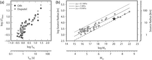
Scaling laws: (a) comparison among our T_PL estimates and the expected theoretical half-duration of the source. Black circles are the theoretical duration estimates computed as 1/2f_c, where f_c is the expected corner frequency using the formula of Hanks & Thatcher (1972) and assuming the stress drop values of Oth (2013). Grey squares are the expected half-rupture duration estimates, according to the empirical scaling relationships of Duputel et al. (2012). (b) Scaling between the length estimates and magnitude for all the analysed events (grey circles) and for the 2000, Tottori event (black star). The dashed lines represent the theoretical scaling, with constant stress-drop value (0.1, 1 and 10 MPa).

Open in new tabDownload slide

RESULTS AND DISCUSSION

The proposed method is a remarkably simple and straightforward approach to rapidly estimate (e.g. automatically, from the real-time data streaming) two main source parameters, the earthquake magnitude and the expected length of the rupture. Earthquake source parameters are generally computed off-line, through fairly complex procedures, mainly performed in the frequency domain. The seismic moment, for example, is estimated from the low frequency amplitude of displacement spectra. The source radius is typically obtained from the spectral corner frequency (Brune 1970; Madariaga 1976) or from time-domain, source duration measurements, generally available several minutes after the earthquake occurrence (Boatwright 1980; Duputel et al.2012). The proposed methodology aims at the real-time, automatic determination of source parameters and it is based on the continuous measurement of P-displacement amplitude and the unique pieces of information needed are the earthquake location coordinates. These are used, indeed, both to correct P_d for the geometrical/anelastic attenuation effect and for setting the limit of the PTW for the parameter measurement. Advanced techniques for the real-time earthquake locations have been already proposed and long proven to provide reliable estimates of the source position within few seconds from the first P-wave detection (e.g. Satriano et al.2008).

Despite of its simplicity, the proposed approach is able to provide reliable and accurate estimates of the expected magnitude. The magnitude, indeed, is well reproduced, with an average error with respect to the true magnitude of about 0.1 units. In addition to the magnitude estimate, the methodology also provides reliable estimates of the rupture extent. We found an estimate of the source radius a of about 0.8–3 km for a M 4–5 event; 7–20 km for M about 6–7, while about 80–100 km are expected for M 8–8.5 event (Fig. 2b). These values are indeed of the same order of those expected for a circular rupture model, assuming a constant stress drop scaling. We note that for the M 9.0, 2011 Tohoku-Oki earthquake, both magnitude and length are underestimated with our technique; this result will be discussed later.

The rupture extent represents a key parameter for the correct prediction of the ground shaking at target sites, especially for very large earthquakes, for which the rupture propagates over long distances and the directivity effect and distance attenuation from the finite fault cannot be neglected. The source directivity modulates the amplitude and frequency content of the radiated seismic wave field as a function of the azimuth from the propagating rupture. The knowledge of the expected rupture length and orientation improves the accuracy in predicting the azimuthally varying ground motion amplitude during moderate to large earthquakes. Furthermore, in the near source range, the effects of the finite fault may be relevant and a different metrics for the distance computation needs to be adopted when empirical attenuation relationship are used for ground shaking prediction. The rapid modelling of the finite fault is crucial to assess the earthquake impact and for producing refined and realistic strong motion shake maps, which represent a valuable resource both for the scientific community and for the public, for the efficient planning of emergency operations. In this context, Rhie et al. (2009), developed a methodology to obtain PGV maps from geodetic finite-source models, within 30 min from the earthquake occurrence. A similar approach is represented by the fast kinematic inversion of the rupture process, as proposed by Dreger et al. (2005), who developed a technique that first inverts regional broadband data for finite-source model parameters, and then uses these parameters to include rupture finiteness and directivity in the prediction of the expected shaking distribution. The proposed methodology aims at providing rapid rupture length and average fault slip (through the seismic moment) estimations which can be used, as initial reference values during automatic, waveform inversion methods to retrieve a kinematic source model of the ongoing earthquake rupture.

Our magnitude and rupture length estimations follow a self-similar, constant stress-drop scaling, as shown in Fig. 2(b), where the dashed lines represent the theoretical scaling, computed by assuming constant stress drop values. The available moment magnitude and source radius estimates allow to determine the static stress drop (⁠|$\Delta \sigma = \frac{7}{{16}}\frac{{{\rm M}_{\rm O} }}{{{\rm a}^{\rm 3} }}$|⁠, Keilis-Borok 1959). The static stress drop represents an important parameter for ground shaking and scenario simulations (Baltay et al.2013), since it affects the high-frequency content of ground motion (Brune 1970, 1971; McGuire & Hanks 1980). We observe that stress drop estimates for individual earthquakes range between 0.1 and 13.5 MPa, with a median value of 0.71 MPa. Such an interval is consistent with what has been found by Oth (2013) from the massive analysis of a database of events in the same source region. Our stress drop values do not show a significant variation with seismic moment, over the analysed magnitude range (Fig. S3 in the Supplementary Material).

In terms of real-time applications, several factors still need to be evaluated, to understand how fast and accurately one can reproduce the results of the off-line analysis, in order to implement it as an efficient algorithm in an EEW method. The LPDT curves in our analysis result from the average of hundreds of recording stations, distributed over wide azimuth and distance ranges. In real-time, the availability of data is controlled by the source to receiver geometry. To evaluate the real-time performance, we should simulate the continuous data streaming, accounting for the P-wave propagation through the seismic network. The analysis of the real-time performance of the proposed method requires massive waveform play-backs and it is beyond the purpose of the present work. However, we can theoretically compute the time at which the measurements of parameters PL and T_PL could be potentially available at the Japan strong motion network, assuming a real-time data streaming.

The results are shown in the right lateral scale in Fig. 1(d): in a simulated real-time mode, about 1–2 s would be required for M 4–5, 3–10 s for M 6–7 and 30–40 s for M 8–8.5.

As a case study, we discuss here the application of the proposed methodology to the M 7.2, 2000 Tottori (Japan) earthquake, which was not included in the database used for calibrating the methodology. The average LPDT curve for this event is shown in Fig. 1(b) with coloured circles, while the light grey squares show the single curves for each recording station. We used stations up to a distance of about 200 km and the number of data that contribute to the average is shown with a colour scale. The black stars in Figs 1(c), (d) and 2(b) show the estimates of PL, T_PL and the corresponding source length. In the off-line analysis (i.e. using all the available stations), for the Tottori case, about 34 s from the earthquake occurrence would be available to get the estimate of T_PL. For the same event, if we used only stations within 100 km, the resulting curve (shown as a solid purple curve in Fig. 1b) would have approximately the same shape, but the plateau level would be available only 24 s after the origin time.

For the real-time implementation of the proposed approach, the major difficulty is the development of a robust algorithm for the automatic measurement of T_PL. The fitting procedure with the piecewise model is instantaneous and simple. The challenge is to automatically identify when the LPDT curve becomes stable, without confusing a possible intermediate flattening, with the final plateau level, so producing an underestimation of the magnitude and rupture length.

The most critical issue of the proposed methodology is to assume a triangular shape to represent the source function. The circular fault model of Sato & Hirasawa (1973) is widely used in seismology to model the rupture of small earthquakes (generally, with magnitude smaller than 6.5) and it allows for a simple analytical relationship between the whole rupture duration and the time at the peak of the apparent source time function. Recently, Duputel et al. (2013) analysed the catalogues that provide the point-source parameters of world-wide earthquakes of M_w ≥ 6.5 between 1990 and 2012. Assuming an isosceles-triangular MRF, they showed that the centroid time-delays (i.e. the difference between the MRF peak-time and the rupture nucleation time) can be used as a reliable proxy for the half-duration of the event (see fig. 2a of Duputel et al.2013). By adopting the Sato & Hirasawa (1973) model we made the basic assumption of a triangle-like, apparent source time functions whose peak-time and total durations are controlled by the rupture end-points, the closest and farthest to the observer, respectively. However, to support our assumption, we compared the observed peak-time values (T_PL) with the half-duration estimates obtained by the empirical scaling relationship of Duputel et al. (2013) (T_Duputel, see Text S3 in the Supporting Information) and show that they provide very consistent estimates in the whole analysed magnitude range. This assumption of a circular fault model can be inadequate to describe the complexity of the source for large events, for which multiple peaks of moment release can occur. This is, indeed, the case of the M 9.0 Tohoku-Oki event, for which our magnitude estimation provides a value of about 8.4. For this earthquake, the rupture history has been shown to be complex and frequency dependent, with three different slip episodes radiating energy in different frequency bands and appearing as three principal peaks in the MRF function (Lee et al.2011; Meng et al.2011; Maercklin et al.2012). The plateau level on our LPDT curve around 30 s corresponds to the end of the first rupture episode; longer P wave time windows should be used to observe the following phases of slip release (Colombelli et al.2012). A further discussion about the use of the circular model is reported in Text S4 of the Supplementary Material.

Minor limitations of the proposed methodology can be related to a non-homogeneous azimuthal coverage of recording stations, which can result in under/overestimations of the LPDT curves, with consequent biased estimates of M, L and Δσ.

Finally, effective tsunami early warning generally requires alert notification within 5–15 min from the earthquake occurrence. Automatic methods for recognizing earthquakes with a high tsunamigenic potential have been recently proposed by Lomax & Michelini (2009a,b, 2012). These are based on a duration-amplitude measurement and on an exceedance criteria that can be completed within 3–10 min after the earthquake occurs, to identify large or devastating tsunamis. Within this context, the independent measurements of magnitude and rupture length, as resulting from our methodology, could also allow for a rapid evaluation of the average slip on the fault (Text S5 and Fig. S3 in the Supplementary Material) which can be used as an additional discriminant for tsunami potential, associated to large magnitude earthquakes occurring offshore. Our method could be a valuable complementary approach for a first-order discrimination between a small-magnitude event and the occurrence of a large earthquake, and can facilitate and speed the release of tsunami warnings.

We acknowledge the Japanese National Research Institute for Earth Science and Disaster Prevention (NIED) for making the Kik-Net and K-net strong motion data accessible through website (http://www.kyoshin.bosai.go.jp/). The authors wish to thank Norm Sleep and an anonymous reviewer for their comments about this manuscript. This work was financially supported by a Post-Doctoral Fellowship at the University of Naples, Federico II and by AMRA scarl, through EU-FP7, in the framework of project REAKT.

REFERENCES

SUPPORTING INFORMATION

Additional Supporting Information may be found in the online version of this paper:

Text S1. Data set description.

Text S2. Description of data processing.

Text S3. Theoretical source duration computation.

Text S4. Circular fault model assumption.

Text S5. Average slip computation.

Figure S1. Data. The map shows the distribution of stations used in this study (small grey circles) and the epicentral location of the 43 selected events (coloured stars). The size of the star is proportional to the magnitude and the colour represents the source depth.

Figure S2. Fit model. Schematic representation of the piecewise linear fitting function, redrawn by Colombelli et al. (2014). In this model, PL represents the saturation level of LPDT curves and TPL the corresponding time.

Figure S3. Average slip and stress drop versus Magnitude. (a) Average slip values obtained by TPL estimates, for each magnitude in our database. Given the estimate of the source radius a, the average slip is computed as Δu = M₀μ Σ, where M₀ is the seismic moment, μ is the rigidity modulus and Σ is the area of the circular fault. (b) Stress drop values for each event, as a function of magnitude.

Figure S4. Comparison of duration estimates. Light grey circles are the observed peak-time values (TPL) while dark grey squares are theoretical half-duration estimates obtained by the relationship of Duputel et al. (2013).

Table S1. List of the analysed events.

Table S2. Coefficients of eq. (2) for each magnitude (and distance range) (Supplementary Data).

Please note: Oxford University Press is not responsible for the content or functionality of any supporting materials supplied by the authors. Any queries (other than missing material) should be directed to the corresponding author for the paper.